UNIVERSITÉ DU QUÉBEC
MÉMOIRE PRÉSE TÉ
À L'
UNIV
ERS
ITÉ DU QUÉBEC
À TROIS-RIVIÈRES
COMME EX
IG
ENCE
PARTIELLE
DE LA
MAÎTRISE
EN GÉN
IE ÉLECTR
IQ
UE
PAR
ABDELRAHMAN
YOUSIF
ESHAG
LESA
COMMANDE
VECTORIELLE SANS CAPTEUR
PAR
PROCESSEUR NUMÉR
IQ
UE
DE LA MACHINE
ASYNCHRONE
Université du Québec à Trois-Rivières
Service de la bibliothèque
Avertissement
L’auteur de ce mémoire ou de cette thèse a autorisé l’Université du Québec
à Trois-Rivières à diffuser, à des fins non lucratives, une copie de son
mémoire ou de sa thèse.
Cette diffusion n’entraîne pas une renonciation de la part de l’auteur à ses
droits de propriété intellectuelle, incluant le droit d’auteur, sur ce mémoire
ou cette thèse. Notamment, la reproduction ou la publication de la totalité
ou d’une partie importante de ce mémoire ou de cette thèse requiert son
autorisation.
Abstract
The squirrel cage induction machine characterized by its simplicity of construction, robustness and low cost, is the workhorse of industry. However, the control of such machine is quite complex. This is due to the coupling between the torque and flux producing mechanisms. Recently, variable speed drives incorporating a1temating CUITent (AC) machines have been taking place over the direct current (OC) ones as a resuIt ofthe progress in the tield of power electronics and digital signal processing (DSP) technology where several control techniques emerged. These techniques, such as vector control, allow a precise and instantaneous torque and speed control of induction machines for high performance applications.
Generally, a speed sensor is used to measure the machine speed for vector control purposes. Speed sensors degrade system reliability particularly in hostile environments. ln sensorless control technique, the speed sensor is replaced by a speed estimator, whkh eliminates the costs associated with the speed sensor and reduces the drive complexity. The purpose of the present research work is to design and implement an induction machine sensorless vector control using a digital signal processor and to evaluate its performance. A digital tilter is used to tilter motor currents. The tilter implementation reduces the drive cost since it is a part of the vector control algorithm.
To achieve the research objectives, modelling of the drive main components are carried out, basically the induction motor and the inverter. Both, steady state and dynamic models of the induction motor are discussed. Matlab-Simulink software is used to simulate a variable speed drive using the direct vector and sensorIess control techniques. At the end, a typical electric drive using eZdspF2812 evaluation board is developed. The simulation and experimental results obtained are good enough to say that this research project accomplished successfully its goals.
Résumé
La machine à induction à cage d'écureuil, qui se caractérise par sa simplicité de construction, robustesse et faible coût, est couramment utilisée dans l'industrie moderne. Ces avantages rendent ce type de machine un choix populaire pour réaliser des entraînements électriques performants où, traditionnellement, seules les machines (CC) étaient uti 1 isées. Toutefois, la commande d'une machine à induction est très complexe [1 ]. Récemment, les entraînements à vitesse variable incorporant des machines asynchrones ont pris le dessus en raison du progrès dans le domaine de l'électronique de puissance et de la technologie de traitement numérique du signal où plusieurs techniques de commande ont émergé. Dans le passé, des telles techniques de commande n'auraient pas été possibles en raison de la complexité du matériel et des logiciels nécessaires pour résoudre le problème complexe de la commande [3].
En général, la vitesse de la machine est mesurée pour l'utiliser comme un signal de rétroaction dans la boucle de contrôle de vitesse de la commande vectorielle. Les capteurs de position et de vitesse diminuent la fiabilité du système particulièrement dans les environnements hostiles. Dans la technique de commande sans capteur, le capteur de vitesse est remplacé par un estimateur de vitesse qui élimine les coûts associés au capteur de vitesse et réduit la complexité de l'entraînement [5].
L'objectif de ce travail de recherche est de concevoir et de réaliser la commande vectorielle d'une machine asynchrone (sans capteur) en utilisant un processeur numérique de signal (DSP) et d'en évaluer la performance. Le travail vise aussi à concevoir et implémenter un filtre numérique dans l'algorithme de commande sans capteur pour filtrer les courants mesurés de la machjne.
Le travail commence par une recherche bibliographique. Ensuite, nous effectuons la modélisation et la simulation de la commande vectorielle dans l'environnement Matlab/Simulink/SimPowerSystems. Par la suite, nous développons un algorithme de commande permettant d'introduire un filtre numérique. Enfin, la validation expérimentale est effectuée. 1
Acknowledgements
1 am heartily thankful to my supervisor, Mamadou Lamine DOUMBIA and my co-supervisor, Pierre SICARO for their encouragement, guidance and support throughout my research project.
It is a pleasure to thank Sebastien DULAC and Francois LABARRE for their cooperation.
1 am grateful to my friend Brahim 1 for the valuable discussions and the time we spent together.
Finally, 1 owe my deepest gratitude to my family for their uItimate support.
Table of Contents
Abstract
...
...
...
...
...
i
Résumé
..
...
...
...
...
...
...
...
...
...
...
...
..
...
ii
Acknowledgements
...
...
...
...
..
...
....
..
.
iii
Table of Contents
...
...
...
...
...
...
..
...
... iv
List of Figures ...
...
..
...
...
...
...
viii
List of Symbols
...
...
... xi
Chapter 1- Introduction ...
...
...
..
...
..
.. 1
1.1 Background ... 1 1.2 Research problem ... 2 1.3 Objective ... 4 1 .4 Methodology ... 4 1.5 Thesis overview ... 4Chapter 2 -
Induction motor modelling
...
..
...
6
2.1 Introduction ... 6
2.2 Steady state Model ... 7
2.3 Dynamic Model ... 8
2.4 Simulation ... 1 1 2.5 Conclusion ... 14
Chapter 3 - Induction motor control..
... 15
3.1 1 ntroduction ... 15 Scalar control ... 15 3.2 3.2.1 3.2.2 Stator Voltage Control ... 15Voltage /frequency (V-f) control ... 15
3.3 Vector control ... 16
3.3.1 Direct FOC ... 16
3.3.2 Indirect FOC ... 17
3.4 Direct torque control ... 18
3.5 Space Vector Pulse Width Modulation ... 19
3.6 Simulation of direct vector control ... 22
3.7 Discussion: ... 26
3.8 Sensorless Control ... 27
3.8.1 Open loop estimators ... 28
3.8.2 Model Reference Adaptive Systems ... 31
3.8.3 Adaptive Observer ... 34
3.9 Simulation of sensorless vector control ... 36
3.10 Conclusion ... 39
Chapter 4 - Digital Filters ...
...
40
4.1 Introduction ... 40
4.2 Types of digital filters ... 4\
4.2.1 Finite impulse-response (FI R) ... 4\
4.2.2 Infinite impulse-response (IIR) ... 41
4.2.3 Recursive realization ... 41
4.2.4 Non-recursive realization: ... 41 4.3 FIR advantages ... 42 4.4 Filter design ... 43 4.4.1 Response ... 43 4.4.2 Specification ... 43 4.4.3 Design method ... 43 4.5 FIR Implementation ... 47 4.6 Conclusion ... 49
Chapter 5 - DSP based Implementation ... 50
5.1 Introduction ... 50
5.1.1 Key Features of the eZdspTM F2812 ... 50
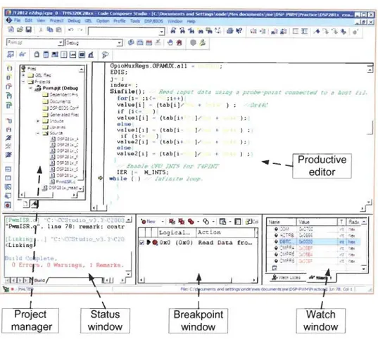
5.2 Code Composer Studio ... 51
5.3 Generation of sine modulated pulse width modulation signaIs ... 53
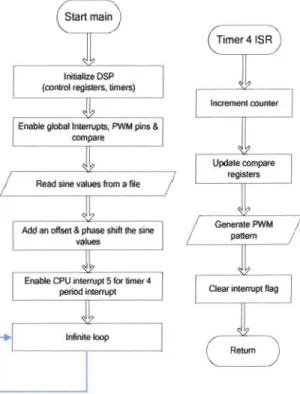
5.3.1 DSP SIGNAL GENERATION METHODOLOGY ... 54
5.3.2 Code generation ... 54
5.3.3 Experimental resuIts ... 60
5.3.4 Discussion ... 63
5.4 Sensorless vector control ... 64
5.4.1 PWM interface circuit ... 66
5.4.2 Current amplification circuit ... 67
5.4.3 Software Implementation ... 69
5.4.4 Speed measurement ... 73
5.4.5 Experimental Results ... 75
Chapter 6 - Conclusion ...
..
...
...
...
...
..
..
....
...
..
...
...
... 79
References
..
...
....
..
...
....
....
...
...
..
...
...
..
..
..
...
....
...
..
...
..
... 81
Appendices ... 83
A- Résumé du travail de recherche ... 83
B- Sinusoidal PWM Code ... 105
C- Sensorless vector control Code ... 108
D- SVPWM Matlab Code ... 120
E- Simu1ated Machine parameters ... 122
List of Figures
Figure 2.1 Winding arrangement of a squirrel-cage induction motor ... 6
Figure 2.2 Per-phase equivalent circuit in steady state ... 7
Figure 2.3 dq-winding equivalent circuits ... Il Figure 2.4 Induction Machine Model in Matlab/Simulink ... 12
Figure 2.5 Motor speed ... 12
Figure 2.6 Electromagnetic Torque ... 13
Figure 2.7 Stator current ... 13
Figure 3.1 Direct FOC of an induction motor ... 17
Figure 3.2. Indirect FOC of an induction motor ... 18
Figure 3.3. DTC of induction motor ... 18
Figure 3.4. Three phase inverter connected to an induction motor ... 19
Figure 3.5. SVPWM Switch states ... 20
Figure 3.6. Reference vector Vref is in the 3° sector ... 20
Figure 3.7. Matlab/Simulink model ofSVWPM inverter ... 21
Figure 3.8. SVPWM Inverter output phase voltage ... 21
Figure 3.9 Direct vector control overall structure-Simulink model... ... 22
Figure 3.10. Current model block ... 23
Figure 3.1 1 Control 1er block ... 23
Figure 3.12. Direct vector control speed response ... 24
Figure 3.13. Direct vector control torque response ... 24
Figure 3.14. Direct vector control- stator current... ... 25
Figure 3.15. Direct vector control rotor position ... 25
Figure 3.16. Open-Ioop rotor speed estimator ... 29
Figure 3.17. Open-Ioop estimator -Simulink model ... 29
Figure 3.18. Open-Ioop estimator speed ... 30
Figure 3.19. Zoomed Open-Ioop estimator speed ... 30
Figure 3.21. MRAS-based speed estimator ... 31
Figure 3.22. MRAS-based speed estimator- Simulink model ... 32
Figure 3.23. MRAS-based estimator speed ... 32
Figure 3.24. Zoomed MRAS-based estimator speed ... 33
Figure 3.25 MRAS-based estimator flux angle ... 33
Figure 3.26. Overall sensorless control structure -Simulink model ... 36
Figure 3.27. Adaptive speed observer-Simulink modeL ... 36
Figure 3.28. Sensorless vector control speed response ... 37
Figure 3.29. Sensorless vector control Estimated vs. Measured speed ... 37
Figure 3.30. Sensorless vector control torque response ... 37
Figure 3.31. Sensorless vector control - Stator current ... 38
Figure 3.32 Sensorless vector control flux angle ... 38
Figure 4.1 Digital filter block diagram ... 40
Figure 4.2 FIR tilter diagram ... 42
Figure 4.3 Filter design flow chart ... 45
Figure 4.4 FDA Tool Graphical User Interface ... 45
Figure 4.5 1 mpulse response ... 46
Figure 4.6 Step response ... 46
Figure 5.1 eZdsp F2812 block diagram ... 51
Figure 5.2 Code Composer Studio ... 52
Figure 5.3 Three phase sine wave modulating signaIs ... 55
Figure 5.4 DSP signal generation flowchart ... 57
Figure 5.5 PWM patterns at 5 kHz and 10 kHz ... 60
Figure 5.6 Voltage waveforms at 5 kHz and 10 kHz ... 61
Figure 5.7 CUITent waveforms at 5 kHz and 10 kHz ... 61
Figure 5.8 Voltage harmonies values at 5 kHz and 10 kHz ... 62
Figure 5.9 CUITent harmonies values at 5 kHz and 10 kHz ... 62
Figure 5.10 Voltage and CUITent harmonies spectra at 5 kHz and 10kHz ... 63
Figure 5.11 Hardware configuration ... 65
Figure 5.12 PWM interface circuit ... 66
Figure 5.13 Current measurement and amplification circuit ... 67
Figure 5.14 Amplifier output ... 68
Figure 5.15 Amplifier input ... 68
Figure 5.16 Algorithm flowchart ... 69
Figure 5.17 Vector control algorithm ... 71
Figure 5.18 Speed measurement Block diagram ... 73
Figure 5. J 9 Speed measurement Front Panel ... 74
Figure 5.20 Phase (A) cuITent ... 75
Figure 5.21 Estimated rotor flux angle ... 75
Figure 5.22 Reference and Estimated speed -0.6 P.u ... 76
Figure 5.23 Reference and Estimated speed - 0.3 P.u ... 76
Figure 5.24 Speed response ... 77
Figure 5.25 Reference and measured speed ... 77
Subscripts s r a,b, C A,B, C d, q 1 m m ag Superscripts a, b, c A,8,C 1\ Symbols V, v l, i R L X E,e S À, \If
e
Stator Rotor Stator phases Rotor phases dq-winding Leakage Magnetizing Mechanical air gap Stator phases Rotor phases Space vector Estimated Value Voltage CUITent Resistance Inductance ReactanceList of Symbols
Back electromotive force Slip
Flux
Angle or position
(û Angular velocity, speed
cr Leakage factor
Tem Electromechanical Torque
TL Load torque
p Number ofpole pairs
T
r Rotor time constants Derivative
Pm Mechanical Power
(ûs Speed of revolving field, in rads (Ûr Speed of rotor, in rads
kj Integral gain
Chapter 1- Introduction
1.1
Background
An electric drive is an electromechanical system that performs the conversion of electrical energy into mechanical energy for the operation of technological processes.
Today, in industrialized countries, over 60% of the electrical power destined to the industry, is consumed by electric drives. Therefore, electric drives that require precise control of torque, speed and position are widely spread. Such drives are characterized by fast torque response and controllability of torque and speed over a wide range of operating conditions [1). Industrial electric drives are generally classified into constant
speed and variable speed ones. Traditionally, Altemating Current (AC) machines were used in applications with constant speed, while separately excited Direct Current (OC) machines were preferred for variable speed applications, because their control is simple and has a very fast torque response. However, DC machines, in addition to their high cost, have also maintenance problems associated with commutators and brushes, which limit machine operation in dirty and explosive environments [2).
The squirrel cage induction machine, characterized by its simplicity of construction,
robustness and low cost, is commonly used in modem industry. These advantages made this type of AC machine a popular choice to achieve modem high performance electric drives for applications where traditionally only OC motors were applied. However, the control of such induction machines is quite complex. This is due to the fact that the rotor current in an induction machine, which is responsible for the torque production, owes its origin to the stator cUITent, which also contributes to the air-gap flux, resulting into a coupling between the torque and flux producing mechanisms [1]. Recently, variable speed drives incorporating altemating CUITent (AC) motors have been taking place over the direct CUITent (OC) ones as a result of the progress in the field of power electronics
and digital signal processing (DSP) technology where several control techniques emerged. In the past, such control techniques were not possible because of the complexity of the hardware and software needed to solve the complex control problem [3].
The appropriate control method of an induction machine is chosen depending on the required performance level. When the dynamic performance is not crucial as in the case of pumps, fans and compressors, relatively simple control techniques are used, which are
generally called scalar control. But when dynamic performance is essential, it is necessary to control the torque at low speeds and during transients. Basically, there are
two types of instantaneous torque control used for high performance applications; direct torque control and field oriented control, named also vector control [4]. Yector control is one of the techniques used to precisely control torque and speed of induction machines used in high performance applications. Using space-vector theO/y, it is easy to show that,
similarly to the expression of the electromagnetic torque of a separately excited OC machine, the instantaneous electromagnetic torque of an induction machine can be expressed as the product of a flux-producing current and a torque-producing current, if a special, flux-oriented reference frame is used [3].
1.2 Research problem
Generally, the machine speed is measured and used as a feedback signal in the speed control Joop of vector or direct torque control. Speed or position sensors degrade system
reliability particularly in hostile environments. In sensorless control technique, the speed sensor is replaced by a speed estimator, which eliminates the costs associated with the speed sensor and reduces the drive complexity [5]. The major drawbacks of sensorless control are the constrains associated with the estimation of non measurable quantities (stator and rotor flux) and / or quantities we do not want to measure for economic reasons
(speed, position) [6]. These quantities could be estimated from the easily measured stator voltages and currents. There are many techniques presented in the literature to extract the speed from measured voltages and currents. However, the performance of these
techniques at low speed remains uncertain. A lot of recent research is focusing on developing efficient speed estimation techniques in order to improve low-speed performance of sensorless drives.
The speed estimation techniques are generally classified into three main groups:
• The first includes estimators based on the dynamic model of the induction machine. In this case the flux is deduced from the dynamic equations of the machine [6]. This approach is straightforward, but it is very sensible to machine parameters and there are also problems associated with using integrators to obtain the flux [7]. Because of errors induced by the use of pure integrators, flux estimators who se designs are based on low pass filters have been proposed [8,9]. However, the filters generate phase delays incompatible with the requested dynamics and lead to instability at high speed.
• The second uses the techniques of signal processing to extract the required information. Despite its simplicity, this technique requires complex filtering circuits and its dynamic performance is poor [10, II].
• The third is based on techniques of artificial intelligence (neural networks, fuzzy logic and genetic algorithm). The neural networks estimators seem to have a better response, but their practical implementation remains a challenge [6]. Traditionally, motor control was designed with analog components which are easy to design and can be implemented with relatively inexpensive components. However, the analog components are affected by temperature and aging, therefore the control system needs to be adjusted periodicaIly. Moreover, the design of analog motor control is hardware dependant so the upgrade of su ch system is quite complex. Digital motor control systems provide practical solutions to the analog control drawbacks. Upgrade is easily performed by software and most of the analog components could be replaced by functions. Despite the solutions offered by digital control, the motor control industry faces many challenges such as power consumption reduction and Electromagnetic interference (EMI) reduction issues imposed by govemments. Furthermore reducing the cost is essential for the industry to remain competitive. The results of these constraining factors are the need of enhanced algorithms. DSP technology allows to achieve both, a high level of performance as weil as a system cost reduction [12].
1.3
Objective
The main objective ofthis research work is to design and implement a reliable sensorless vector control of induction machine using a digital signal processor (DSP) and to assess its performance. The work aims also to introduce digital filters into the control structure. To achieve the research goals, several issues will be addressed such as: (a) modelling and simulation of electric drives using Matlab/Simulink; (b) fixed-point digital signal processors and their application in electric drives; (c) digital filtering; (d) real time implementation; (e) LabVIEW interface development.
1.
4
Methodology
The work begins with a literature review (State of the Art) ofvector control and the study of fundamental concepts of different estimation techniques applied to sensorless speed control of squirrel cage induction machines. Then, modeling and simulation of an induction machine as weil as vector control will be carried out in Matlab / Simulink. Furthermore, digital filter will be introduced in the control structure. Finally, we will conduct an experimental validation of the vector control on a test bench.
1.5 Thesis overview
The thesis consists of six chapters. Chapter 1 introduces electric drives, research questions and provides an overview of the thesis. Chapter 2 presents the steady state and dynamic models of the squirrel-cage induction machines. The relevant equations and equivalent circuits are detailed. Dynamic model simulation results are shown where the response of the induction machine could be evaluated. ln chapter 3, the different techniques of the induction machine control are discussed. First, scalar control and its various types are discussed. Then direct torque control is reviewed. Both mentioned control types are dealt with in a qualitative way. However, field oriented control and estimation techniques are discussed in details followed by the simulations results.
In chapter 4, digital filter types, characterization, analysis techniques and design aspects are addressed. Then, details ofthe filter used in the drive simulation and its design steps using Matlab filter design and analysis tool (FDAtool) are presented.
The experimental setup is detailed in the chapter 5, including the eZdsp board with the interface and current amplification circuits. A brief description of the Texas Instruments DSP platform (Code Composer Studio) is presented, in addition to the sensorless control implementation. Chapter 6 presents the conclusions of the research and gives recommendations for further research and development work.
Chapter 2 -
Induction motor modelling
2.1 Introduction
ln this chapter, induction machine modelling is discussed, since obtaining the mathematical model that characterizes exactly the machine is primordial for motor control purposes. Both steady state and dynamic models are introduced. Finally, the developed Matlab-Simulink model and the simulation results are presented. For analysis purpose, the squirrel-cage on the rotor is replaced by a set of three sinusoidally distributed windings. Winding arrangement for a 2-pole, 3-phase, symmetrical squirrel-cage induction machine is shown in figure 2.1 [13] [14]. The stator and rotor are assumed to have the same number oftums.
1--"::::'--l+-r--'''-1+- - - ' -a -a x i s
al
~
+
Va + ~/ le b)2.2 Steady state Model
When the stator of an induction machine is supplied from a balanced three phase sinusoidal power source and a constant load torque, the equivalent circuit of the induction machine is derived from the concept ofa "rotating transformer" [15]. A diagram of the equivalent circuit with the rotor elements retlected into the stator for a polyphase induction machine is shown in figure 2.2. Core-Ioss resistance is neglected.
Stator and rotor phase voltage equations are drawn from figure 2.2 as follows:
SE
ag =RJ; +
jSX
,J;
Mechanical Power equation:Electromechanical Torque:
Where
s
OJ s - OJ rOJ s
1
;
Figure 2.2 Per-phase equivalent circuit in steady state
7 (2.1 ) (2.2) (2.3) (2.4) (2.5)
R;
s
2.3 D
ynam
i
c M
o
del
The equivalent circuits, derived from steady state operation with sinusoidal voltages and currents, are inadequate when dealing with transients or wh en the motor is supplied from a switched converter [16]. Therefore the steady state equations written in phasor representation are not applicable under dynamic conditions. Instead space vector representation is used to write the machine equations.
Per-phase voltage equations are expressed as:
(2.6)
0
=
Ri
A
(t)
+!!.-
X
A
(t)
r r
dt r
(2.7)Flux linkage equations:
(2.8)
x
:
(t) =
Lm~
A(
t)+
Lr~
A(t)
(2.9)Equations (2.6)-(2.9) constitute the space-phasor model of a squirrel cage induction
machine.
We notice that in (2.8) the rotor current space vector is defined with respect to the stator phase-a axis, meanwhile the stator current in (2.9) is defined with respect to the rotor phase-A axis.
[t is clear that the flux linkage depends on the rotor position for given values of the stator and the rotor currents at any instant of time. For this reason, the voltage equations in phase quantities, expressed in a space vector form by (2.6) and (2.7), which include the time derivatives of the flux linkage, are complicated to solve. This coupling could be avoided by using dq-analysis.
At any instant oftime, the air gap mmfdistribution produced by three phase windings can also be produced by a set of two orthogonal windings, one winding along the d-axis, and the other along the q-axis.
The dq winding analysis allows the torque and the flux in the machine to be controlled independently under dynamic conditions.
Any three-phase sinusoidal set of quantities can be transformed to an orthogonal reference frame by the following transformation matrix:
Id
t
_
2
3
\.
3
.
( )
[
.
()]
( )H
cos(e)
cos(e
-
27l)
coi
e-
47l)
[i
a
(t)]
- - lb
t
i
t
3
2
7l
47l
(2.10)q
-sin(e)
-Sin(e-J
)
-sin(e-
J
)
dt)
Now we can formulate stator and rotor windings equations along two orthogonal axes d
and q moving at speeds (f) d and (f) dA respectively:
Stator windings:
V sd
=
R sisd+
~
ÀSd - {ùdÀsqdt
Rotor winclings: 9 (2.11 ) (2.12) (2.13) (2.14)Where (j) d and (j) dA are the instantaneous speed of the dq-winding set in the air gap
with respect to the stator and rotor axis respectively. Assuming an arbitrary value for the
dq-winding speed with respect to the stator axis, OJ d determines the reference frame,
either stationary ( OJ d
=
0
)
,
stator ( (j) d=
(j) syn ) or rotor ( (j) d=
(j) m ) [13]. Electromagnetic torque: (2.15) ~echanical speed:d
T:m
-TL
- (j)=
--"'-"'---"-dt
mechJ
eq (2.16) OJ elec OJmech*
P
(2.17)The dq-equivalent circuit is obtained by substituting for flux linkage derivatives into
voltage equations (2.1 1 )-(2.14). These equations are in a general reference frame.
Vsd
=
RJsd - {j)dAsq+
L,s~iSd
+
Lm~(i
s
d
+
i rd )dt
dt
(2.18)(2.19)
Rotor windings:
(2.20)
(2.21 )
For each axis, the stator and the rotor windings are combined to result in the dq
R
s OJQ
dÂsq ~L
---/\/\/'v-
c:r-:- . . .
.
--=---
+
+
lsd~d
-
d
Â
ddt
S a) d-axisR
OJ
d
Â
sd
L
---
~
-
~
+
~+
l
sq
~q
d
- Â
sqdt
b)q-axisd
- Â
rddt
d
-
Â
rqdt
Figure 2.3 dq-winding equivalent circuits
2
.
4 Simulation
+
Vr
d
V
rq
The dynamic model equations (2.18) - (2.21) together with the motion equations (2.15) -(2.17) were used to develop a squirrel cage induction model in Matlab-Simulink.
The stator is selected as reference frame (
ru
d=
ru
syn ), therefore (ru dA
=
ru
syn -ru
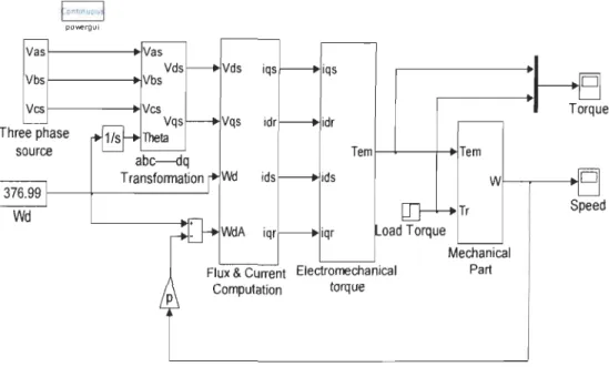
m ). Figure 2.4 shows the developed model in Simulink.FontJnuou~ pOYiergui vasf---~Vas Vds V b s f - - - - ---+lVbs Vcsf---+I Three phase source Torque Tem f--l.--+-~Tem oad Torque Flux & Current Eleclromechanical
Computation torque
Wf--~-~D
Mechanical
Part
Speed
Figure 2.4 Induction Machine Model in Matlab/Simulink
Figures 2.5, 2.6 and 2.7 show the speed, torque and current responses of the induction
machine dynamic model shown in figure 2.4. At t=0.5s a load torque is applied to the machine and its response is found satisfactory
Mechanical Speed [radIs]
200 1 180 1 1601 140,
i
120 ri
100 ~!
80' 601 40' 201 0 0 -L 0.4 -' 0.5 0.2 "-0.3 L 0.6 0.7 0.8 0.9 Tome [51120 1001 80 60 -40
'---o
0.1 -50 0.44 0.46 0.2 Torque [Nm) - - -Measured Torque 1 - - -Load Torque 0.3 0.4 0.5 0.6 0.7 0.8Figure 2.6 Electromagnetic Torque
0.48 0.5
Stator Current
0.52 lime [51
0.54
Figure 2.7 Stator CUITent
13 0.56 0.9 0.58 '1 0.6
2.5 Conclusion
Squirrel-cage induction machine modelling and simulation is described in this chapter. The traditional per-phase equivalent circuit is presented. Generally, this model is useful in analysing the steady state performance of the induction machine. A dynamic model of the induction machine is developed and the equivalent circuit is introduced. The dynamic model is simulated using Simulink. The machine response to a torque variation is investigated. The dynamic model will be used in the next chapter to develop a Simulink model of an electric drive.
Chapter 3 -Induction motor control
3
.
1
I
ntroduction
This chapter describes various control methods used in induction machine variable speed
drives. First, scalar control techniques based on the steady state model are discussed.
Instantaneous torque control methods, mainly direct torque and field oriented control are presented. Inverter pulses generation method is also described. Finally, sensorless control and various estimation techniques are discussed in detail followed by simulation results.
3.
2 Scala
r
control
The basic techniques of induction machine speed control are elaborated using the
elementary model described in the steady state analysis. These techniques are viable
when the motor operate at steady torque and when small errors in speed control are
tolerated. Several open-Ioop (scalar) control methods are outlined in the literature. Sorne
of popular scalar control methods are detailed below.
3.2.1
Stator Voltage Control
ln this method of speed control, the magnitude of the terminal voltage is varied up to its rated value. A wide range of speed control cannot be accomplished by this
technique. Generally, back-to-back thyristors are used for this purpose but this type of
drive suffers from poor power and harmonic distortion factors when operated at low speed [17].
3.2.2 Voltage Ifrequency (V-f) control
ln this scheme, induction motors are driven from a variable voltage supply with
adjustable frequency. The combination of voltage amplitude and its frequency is
necessary, since increasing the supply frequency alone increases the motor speed but
reduces the maximum motor torque. Furthermore increasing the voltage amplitude alone
increases motor maximum torque. The motor supply voltage amplitude is varied in proportion with its frequency in order to maintain the air gap flux to its rated value [17], [ 18].
3.3 Vector control
It is a control strategy for three phase ac motors that emulates the dc motor control
by orienting the stator CUITent so as to control torque and flux independently. The stator
CUITent components obtained are oriented in phase (flux component) and in quadrature
(torque component) to the flux vector, which can be one of the three distinct flux
space-phasors in the induction machine: airgap, stator and rotor flux. Vector control could be
perfonned with respect to any of these flux space-phasors by attaching the reference
system d axis to the respective flux linkage space-phasor direction and by keeping its
amplitude under surveillance. The rotor flux orientation provides natural decoupling, fast torque response and ail around stability. Stator flux orientation and airgap flux orientation are attractive due to ease of flux computation and for the purpose of wide range of field
weakening, but a decoupler network is needed [1, 19].
Vector control technique allows a squirrel-cage induction motor to be driven with high
dynamic performance, comparable to that of a dc motor. This type of control is suitable
for applications that require accurate control of speed and position. [n vector control, the
dynamic model of the induction machine rather than steady-state model is used to design the controller [17, 19]. There are basically two different types of vector control
techniques. Either direct or indirect field oriented control (FOC), depending upon the method of flux acquisition.
3
.3.
1 Direc
t
FOC
In the direct method, the airgap flux is directly measured with the help of sensors, search
coils or taped stator windings or estimated from machine terminal variables such as stator
voltage, current and speed. Since it is not possible to directly sense rotor flux, it is synthesized from the directly sensed airgap flux. Rotor flux angle is directly computed from flux estimation or measurement.
A major drawback with the direct orientation scheme is the inherent problem at very low
speeds when the machine IR drop dominates and the required integration of the signal to
measure the airgap flux is difficult. Closed-Ioop stator flux observers based on the motor
current, voltage and the measured rotor position have been found to overcome this
To illustrate a rotor flux based direct vector-controlled drive, figure 3.1 shows the schematic diagram of an induction motor drive system with impressed stator CUITents employing direct rotor-flux-oriented control and using a CUITent regulated pulse width modulation inverter (CRPWM) [3].
p
r
Flux
Model
Figure 3.1 Direct FOC ofan induction motor
3.3.2 Indirect FOC
PWM Inverter
(j)
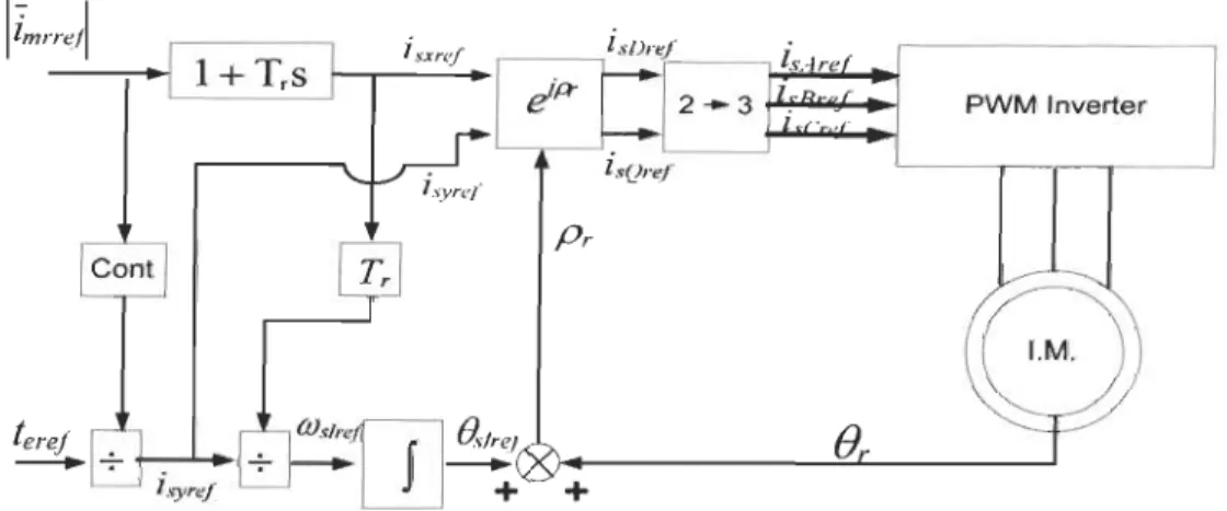
[n this method, the rotor flux angle is indirectly computed by summing a sensed rotor position signal with a commanded slip position. ln contrast to direct methods, the indirect methods are highly dependent on machine parameters, which may vary with temperature,
saturation level and rrequency. Consequently, parameter adaptation schemes are required to have a betler overall performance. Figure 3.2 shows the schematic diagram of an induction motor drive system with impressed stator currents employing indirect rotor-flux-orientation [1, 3]. The speed control loop is not shown, but it is identical to that illustrated in figure 3.1.
PWM Inverter
+
Figure 3.2 Indirect FOC of an induction motor
3
.4 Direct torque control
ln addition to vector control systems, instantaneous torque control yielding fast torque
response can also be obtained by employing direct torque control (DTC) where flux
linkage and electromagnetic torque are controlled directly and independently by the
selection of optimum inverter switching modes. The selection is made to restrict the
flux-linkage and electromagnetic torque errors within the respective flux and torque hysteresis
band, to obtain fast torque response, low inverter switching frequency and low harmonic
losses. Figure 3.3 shows the schematic of a simple form of direct torque control induction
motor drive [3]. The speed control loop is not shown, but it is identical to that illustrated in figure 3.1.
Tor ue Ret. +
Inverter Optimal Switching Table
Electromagnetic torque
+ Flux linkage estimator VSI
r.-:\
Inverter f -... -"T"-1U
v isb3
.
5 Space Vecto
r
Pulse Width Modulation
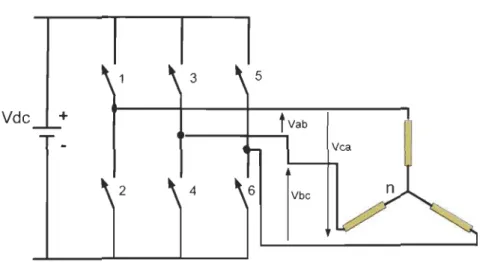
The structure of a typical 3-phase power inverter is shown in Figure 3.4 where Yab, Ybc and Vca are the voltages applied to the motor windings. Vdc is the continuous inverter input voltage. The ON-OFF sequence of ail these devices must respect the following conditions:
1- Three of the switches must al ways be ON and three always OFF.
2- The upper and the lower switches of the same leg are driven with two complementary pulsed signais. In this way no vertical conduction is possible, providing care is taken to ensure that there is no overlap in the power switch transitions [20].
3
Vdc
+
Vca
2 4
n
Figure 3.4 Three phase inverter connected to an induction motor
Space Vector Pulse Width Modulation (SVPWM) is one of the methods to determine
switched pulse width. It is easy to implement and has a good performance concerning harmonic content reduction. Taking into consideration the two constraints quoted above, there are eight possible switch states. Two of these states (Vo and V7) correspond to a
short circuit on the output, while the other six can be considered to form stationary
vectors in the d-q complex plane as shown in figure 3.5 [21].
The reference vector, which represents three phase sinusoidal voltage, is generated using SVPWM by switching between two nearest active vectors and zero vector [22]. Each of
the active six vectors has a magnitude of 4/3 Vdc.
d
(Real)
Figure 3.5 SVPWM Switch states
Assuming that the reference vector V ref is in the 3° sector as shown in Figure 3.6, we have the following situation, where T4 and T6 are the times during which the vectors V4 and V6 are applied and TO is the time during which the zero vectors are applied. When the reference voltage and the sample periods are known, the following system makes it possible to determine the switching times T4, T6 and TO.
(3.1 )
(3.2) A Matlab/Simulink model of SVPWM inverter developed in [22] is used in the vector
control simulation. The switching time and corresponding switch state for each power
switch is caJculated using Matlab code. Figure 3.7 shows the complete inverter model in Simulink. The model is tested by supplying it with d-q reference voltage and the results
are shown in figure 3.8.
Mag Angle Va RefVoltage Generator Vb 200 o
~
Repeating Sequence Vc VabcFigure 3.7 Matlab/Simulink model ofSVWPM inverter
Phase-A \.4Jltage [V] -200 l " -'---~-~--= o 0.005 0.01 0.015 0.02 0.025 0.03 0.035 0.04 0.05 Phase-B \.4Jltage [V) 200 o -200 l J 1 . . . . L L i o 0.005 0.01 0.015 0.02 0.025 0.03 0.035 0.04 0.045 0.05 Phase-C \.4Jltage [V] 200, -'-
,
, 0.015 0.02 0.025 0.03 0.035 0.04 0.045 0.05Figure 3.8 SVPWM Inverter output phase voltage
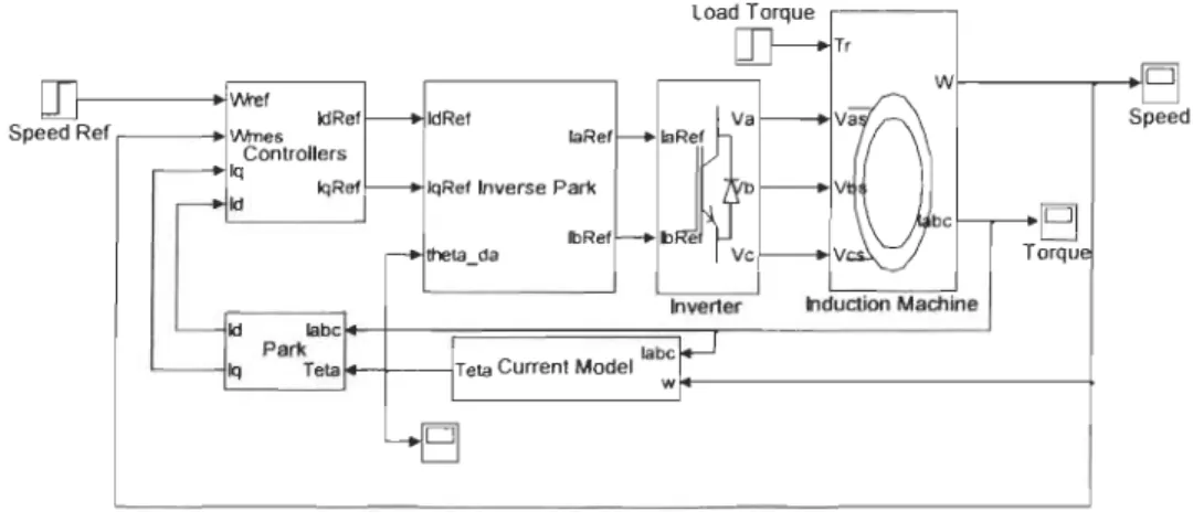
3.6 Simulation of direct vector control
The rotor flux oriented direct vector control technique described in subsection 3.3.1 is
simulated using Simulink. The simulated control structure in shown in figure 3.9 where
the induction machine subsystem contains the motor model developed in chapter two.
The inverter subsystem consists of the SVPWM inverter model detailed in section 3.5
above.
wl---,--.jD
t---+iWref
Speed Ref . - - - ----+1 IaRef
IbRef
11:
f)tc
:
v1J
n
oc
Inverter Induction Machine
1 -+---ITela Current Model labc
~--~ L:~~~~~w~---1
Figure 3.9 Direct vector control overall structure-Simulink model
Speed
The CUITent model block calculates the rotor angle, which is derived from the rotor
voltage equations expressed in the rotor flux oriented reference frame. ln this case, the
entire flux is aligned to the rotor flux, so the quadrature component of the rotor flux
equals zero. Reformulating rotor equations (2.13-2.14), we obtain the new rotor equations shown in (3.3) and (3.5). The rotor angle is calculated using the following equations as shown in figure 3.10.
0
=
Rr
1d
1/I.'d
+ -
/l.rdL
r'
dt
(3.3)0=
R
ri
rq+
((V sys - (V m)Â
rd (3.5)L .
Irq = -~l L sq r (3.6) (Vsl RrxL
m lsq Lr X Ârd (3.7) ()f
(Vm+
(Vsl (3.8) I--~---êl L!..!!.2:!'-'--.l ~~~ labc CD Teta Œ : : ) r - - -+ wFigure 3.10 CUITent model block
The controller block illustrated in the direct vector control structure (figure 3.9) contains
two parallel control loops having Proportional Integral (PI) controllers. The first loop is
used to adjust the machine flux. The second one consists of two cascade loops, the inner
current and outer speed control loops. The controllers are tuned by trial and eITor method.
Figure 3.11 below shows the contents of the controller block.
~~Œ::)--.!=
:
I
:C;::::::=-o~I---.
_
y
Id PI(flux) Œ::) lIIknes~P=·~I
-
(
3- )---+l=
:
P=~+I
__
--+
-
Œ::) PI(speed) Iq PI(current) qFigure 3.11 Controller block
Figure 3.12 through figure 3.15 show the simulation results of the direct vector control. 150 100,. '0 CI) If) 0 =0 ~ "'0 -50f CI) CI) a. CI) -1001 -1501 -200 0 60 40
E
20 Z (1) ~e-
0 0 1 l-I -20l
-40 0 l ' Reference Speed ,. 5 lime [s] - Measured Speed '--r 10Figure 3.12 Direct vector control speed response
: Load Torque
I~l
' - Measured Torque
l ~_~_~ j
5 10 15
lime [s]
Figure 3.13 Direct vector control torque response
«
ë l!! :J ü 400L 1 200 0 -200 --400f 7.95 250~ 2001 ~ 150~ c .2~ 100
~
1 1 50~o
o
, , l~_ ", , 8 R05 8.1 8.15 8.2 8.25 8.3 8.35 8.4 lime [sIFigure 3.14 Direct vector control- stator current
5 10 15
Time [5]
Figure 3.15 Direct vector control rotor position
3.7 Discuss
i
on
:
Different operating conditions were investigated in order to validate the direct vector control model and to demonstrate the effectiveness of the system modeling and simulation. Figure 3.12 shows the reference and actual motor speeds, at t=4s, motor speed is increased from 70 to 120 radis. The speed dip at t=6s is due to load torque augmentation. Electromagnetic torque response is illustrated in figure 3.13. Load torque is increased at t=6s. Despite the presence of torque pulsations, the motor follows
precisely the load torque value. At t=8s, motor speed is reduced from 120 to -100 radis
We notice in both figures that in presence of disturbance the vector control responds adequately and brings back the controlled variable to its desired value. Figure 3.14
3.8 Sensorless
Control
Sensorless vector control is an instantaneous electromagnetic torque control technique applied to variable speed (AC) motor drives where speed estimators and observers are used instead of the costly speed or position sensors. Eliminating speed and position sensors reduces hardware complexity and cost, increases the mechanical robustness and reliability of the drive, and leads to a better noise immunity.
There are many speed or position extraction techniques, some of them are only valid in the steady state. Such techniques could be used in low-cost drive applications not requiring high dynamic performance. Other techniques are applicable for high-performance applications in vector- and direct-torque-controlled drives. Most of these techniques depend on machine parameters. Therefore various parameter adaptation schemes have been proposed in the literature. In an ideal sensorless drive, speed information and control is provided with an accuracy of 0.5 % or better, from zero speed to the highest speed, for ail operating conditions and independently from saturation levels and parameter variations [3].
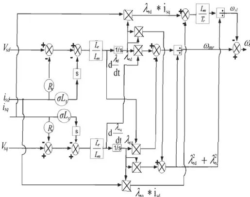
The estimation techniques can be classified into three main groups as detailed below. The first includes estimators based on the dynamic model of the induction machine. The flux is deduced from the dynamic equations of the machine [6] using the monitored stator voltages and currents. The basic scheme is called open-Ioop estimator. This approach is straightforward, but there are problems associated with parameter mismatch
and noise, especially at low speed [7]. Thus it is difficult to achieve stable, very low speed operation in a speed or position sensorless high-performance induction motor drive. Others improved schemes like model reference adaptive systems (MRAS), and observers (Kalman and Luenberger) have better accuracy.
The second uses techniques of signal processing to extract the required information. 1 n one of such estimators, stator currents and spatial saturation third-harmonic voltage are measured and then the fundamental component of the magnetizing flux is determined using the third-harmonic flux. Despite its simplicity, this technique requires complex filtering circuits and its dynamic performance is poor [6].
The third is based on techniques of artificial intelligence (neural networks, fuzzy logic and genetic algorithm). The neural networks estimators seem to have a better response, but their practical implementation remains a challenge [6].
The most popular techniques of sensorless control for induction motor drives are
presented as follows.
3.8.1 Open loop estimators
The monitored stator voltages/currents are used to estimate the flux linkage components,
from which the speed is derived.
The mathematical expression for the rotor speed is given as:
OJ r
=
OJ mr - OJ si (3.9) Where mmr
is the speed of the rotor flux-linkage space vector with respect to the rotor.(3.10)
The angular rotor-slip-frequency (msl) is derived from rotor voltage equation of the induction machine expressed in the rotor flux oriented frame as follows:
{f} si
=
(3.11 )Finally we obtain the speed as shown below:
= Àrd dÀrq /
dt -
Àrq dÀrd /dt
_
Lin (_ 1 1·1 · )
(Or
1-1
21-1
2 /l"rq sd +/I"rd1sqÀr
T
r Àr(3.12)
The implementation of(3.12) is shown in Figure 3.16. First the flux (À) is deduced using
(2.18) and (2.19) in a stationary reference frame (md = 0) as shown in (2.13, 2.14) then (3.12) is used to extract the speed.
Lm
~À
r
d
=
Vs
d
- R
,i
sd
+
L
s
(l-
~J~i
Sd
L
r
dt
LrL~dt
(2.13)Lm
d
1R·
L
(1
L~
J
d
.
- - / 1 "=v
-
l+
-
-
-
- 1L
dt
rq
sq
ss
q
s
L
L
dt
sq
r r s (2.14)ls(~+-t---L...(
lsq
Figure 3.16 Open-Ioop rotor speed estimator
The estimator shown in Figure 3.16 is implemented using Matlab-Simulink as illustrated
in figure 3.17, the motor is supplied from a three phase supply and the measured stator and rotor currents are fed to the estimator as inputs.
kls
Iqs
Figure 3.17 Open-Ioop estimator - Simulink model
r;; ù ~ "0 Q) Q) a. C/') 200 · 50 0 0 191 [ 190 L
i
189
~
1
188r en 187 f. 186 ~ 4 C 1Il 0 '0 ~ -2 -4 0 0.18 T r - Estimated Speed 1 - - : -Measured S~d 1 0.2 0.4 0.6 0.8 lime [sIFigure 3.18 Open-Ioop estimator speed
0.2
r
~
Estimated Speed l' 1 - Measured Speed 0.22 lime [sI 0.24 0.26Figure 3.19 Zoomed Open-Ioop estimator speed
0.1 0.2 0.3 0.4 0.5
lime [sI
Figure 3.20 Open-Ioop estimator flux angle
0.6
The speed response of the open-Ioop estimator is shown in figure 3.18; at motor starting
we notice a smalt overshoot in the estimated speed. Furthermore the zoomed speed
response iltustrated in figure 3.19 shows ripples in the estimated speed, which is a commonplace in such type of speed estimators. Figure 3.20 shows the estimated flux
3.8.2
Mod
el
Refe
r
ence Adaptive Systems
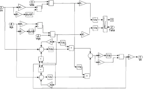
The accuracy of the open loop estimator discussed above depends strongly on the machine parameters. In c10sed loop estimators the accuracy can be increased. In the present section, a closed loop estimator using the Model Reference Adaptive System (MRAS) is described. In a MRAS system, sorne state variables, (e.g. rotor flux-linkage components, or back emf, etc.) of the induction machine are estimated in a reference model and are then compared with state variables estimated by using an adjustable mode!. The difference between these state variables is then used in an adaptation mechanism, which outputs the estimated value of the rotor speed and adjusts the adaptive model until satisfactory performance is obtained [3]. Figure 3.21 shows a complete scheme of MARS-based speed estimator using rotor flux linkages for the speed tuning signal [3). Refèrence model
r--
-
--
----
--
-
---,
J _ Lm ~ ed - ~d"Vs
d
f-i:
_----t.-(
)---~ 1/s1---+----~L, ...., J J J J J J J Ji
s
J J J ~ ---~ Ï..vd adjustable modelFigure 3.2\ MRAS-based speed estirnator
The MRAS speed estimator shown in Figure 3.21 is implemented using Matlab/Simulink
as illustrated in figure 3.22, the motor is supplied from a three phase supply and the
measured stator and rotor currents are fed to the estimator as inputs.
f - - - -
.--.IiK-Ids
1 - r - - - - + --+lK
-Figure 3.22 MRAS-based speed estimator- Simulink model
2001 7il
u
1501
~ 100 -0 Q) Q) 50 a. C/) 0 1 -50 - ---'-0 0.2 04 0.6 0.8 1ïme [s]192
r
1901 (j) =0 188f !!l "0 QI QI 186~
0-C/) 184 ~ r 3r 2t '0 !!l c 0 ~ -1'"
0 CL -2l -3 t 0.2 0.25 Time [51 ...:... Estimated' Speed 1 - Measured Speed 0.3 0.35Figure 3.24 Zoomed MRAS-based estimator speed
-L~~--'----0.1 0.2 0.3 0.4 0.5 0.6
Time [s1
Figure 3.25 MRAS-based estimator flux angle
The MRAS estimator is simulated under the same conditions of the open loop estimator.
Here we notice the absence of the starting speed overshoot found in open loop estimators.
However, the accuracy of the estimated speed is compromised at \ow speed due to the use of pure integrators.
3.8
.
3
Adaptive Observer
A state observer is a model-based state estimator that can be used for the state estimation of a non-linear dynamic system in real time. In the calculations, the states are predicted by using a mathematical model, but the predicted states are continuously corrected by using a feedback correction scheme. Stator and rotor equations of the induction machine in stator coordinates are used to obtain a full-order speed observer [3]. The induction machine equations can be expressed as state variable equations:
d
l
s
A
li
A
12l
s
BI
Iv
s
i
+
dt
À
r
A
21A
22À
r
0
(3.15) Is 1i
d 1 qI
T
v
sI
V
dV
qI
T
(3.16)Àr
À
dr
À qr
I
T
(3.17)AIl
Rr
(1
+
L
2J-
I
m
a
L
L
2 (3.18) s rA
12Lm
(_
1
.
1-
"-.
l
'
J
OJ
ra
L
sL
rT
r (3.19)A
21Lm
. 1
T r
(3.20)A
221
1
+
"-.
l
'
-
- .
OJ
rT
r (3.21 )l
l
'
(3.22)1
-(3.23)
The state observer, which estimates the stator current and the rotor flux together, is
written as
d "
-
X
dt
Where"-A
A IlA
21"
A
12A
22T
B
- - - 1
1
a
L
s (3.24) (3.25) (2.26)The error between the model current and the machine CUITent (is - is) is used to generate
corrective inputs to the dynamic subsystems of the stator and rotor [23]. Hence the
observer gain G is selected so that (3.24) would be stable.
A
-The speed estimator is based on rotor flux /L r and i s estimators
m
r=
(
K
p+
~;
)rrna
g [ (
l
s
-
1,
r
,
]
(3.27)3.9 Simulation of sensorless vector control
The simulation of the sensorless vector control is implemented in Simulink. The structure
of the sensorless electric drive is shown in figure 3.26. The speed observer subsystem
contains the adaptive speed observer model illustrated in figure 3.27. Figure 3.28 through
figure 3.32 show speed, torque, current and position responses of the drive. The motor
parameters are assumed to be constant so parameter variation effects are not investigated.
Ref.Speed
f---.!Ref.w
dt-- ---+ld
ia
q t - - -- Iq Inverse Park Speed & Current
Controllers theta ib dq-ABC Inverter '--..,---lThela vabcl+---' Estim. Observer Flux angle L---r---~W aocl+---~
Estim.speed Speed Observer
Figure 3.26 Overall sensorless control structure -Simulink model
Adapting mechanism
G
Figure 3.27 Adaptive speed observer-Simulink model
Torque
o
Current
CD
150 100
~
, 50 7ii!
0r
Reference Speedri
- - Measured SpeedIl
1
-50 If) -100 -150 ~ - [ 1 -200 '-- ---'--- -'--- -0 5 10 15 Time [s]Figure 3.28 Sensorless vector control speed response
1
::
t
~
~
______
- Ji
01
-50If) -100
~I
-
Measurecl SpeedJ
l
-
Estimated Speed - 1501 1 -2001 o 5 10 15 Time [s)Figure 3.29 Sensorless vector control Estimated vs. Measured speed
60 40 'E' ~ 20~"~ __ ,,~,,,
i
0 -201
-
Load Torqu;l
- Measured Torque i L_ _ _ __ ~ -40 o 5 10 15 Time [s)Figure 3.30 Sensorless vector control torque response
200r 100 ~ ë 0
ê
::> 0 -100 -200 7.9 3 2 ""0 ~ c: 0 0-
fJ) -1 0 a.. -2 -3 5.1-
1-
--,---,-
-r~~1-
-~-~,
r -7.92 7.94 7.96 7.98 8 8.02 8.04 8.06 Time [s]Figure 3.31 Sensorless vector control - Stator CUITent
5.15 5.2
Time [sI
5.25
Figure 3.32 Sensorless vector control flux angle
l
8.08
5.3
The same operating conditions applied to the direct vector control in section 3.7 are applied to the sensorless vector control. The responses in both cases are identical.
3
.1
0 Conc
l
usion
This chapter presented several techniques used to control squirrel-cage induction machines. These techniques prove the controllability of the induction machine in terms of torque, speed and position. The appropriate control technique choice depends on the requested drive performance. If moderate performance fills the application requirements then scalar control techniques is quite enough. Otherwise vector control or direct torque control could be used. Both control techniques provide decoupled flux and torque control.
A senssorless vector control system for induction machine is presented. System modeling and simulation are detailed using Matlab/Simulink. Different flux and speed estimation techniques that could be used in high performance drives were described. Among the presented estimation techniques, the adaptive speed observer has better behaviour with respect to steady state error, parameter sensitivity and dynamic response although its performance at low speed remains problematic. Robust estimation techniques and parameter identification by self-commissioning or by online tuning have the potentiality of reducing the estimation errors. The majority of speed extraction techniques relay on the induction machine mode\.
Chapter 4 -
Digital Filters
4
.1
In
tr
oduction
An electrical filter is a system that can be used to modifY, reshape or manipulate the frequency spectrum of an electrical signal according to sorne prescribed requirements. A tilter may be used to amplifY or attenuate a range of frequency components, reject or
isolate one specific frequency component. Typically, an electrical tilter receives an input
signal or excitation and produces an output signal or response. Depending on the type of
input, output and internai operating signaIs, three general types of tilters can be
identified, namely, continuous-time, sampled-data and discrete-time filters [24].
Depending on the format of the input, output and internai operating signais, filters can be
classified either as analog or digital filters. In analog filters the operating signais are varying voltages and currents, whereas in digital filters they are encoded in sorne binary
format. Digital filters are programmable, reliable and have better performance, in addition to the possibility of implementing complex combinations of filters with
relatively simple hardware requirement. However, they are more expensive compared to
analog ones. Continuous-time and sampled-data tilters are always analog filters, but
discrete-time filters can be analog or digital [24, 25]. A digital filter is used in the
implementation of the sensorless vector control to eliminated measurement noise.
Figure 4.1 shows a digital filter where analog to digital converters are necessary to digitize the unfiltered analog inputs [26]. Then, signal processors are used to implement
digital filters by performing the necessary mathematical operations.
- - -
....
~
unfiltered~
anolog signol s;o'""pl .. d . \ digiti."d :signolPROCESSORI
----
-·~
---
-·
• digÎtolly~
filtared fih .. ,,,d analog ggnol s.ignal4.2 Types of digital fi
l
ters
Mainly, digital tilters are classitied into two types according to tilter characteristics as
shown below [27].
4.2.1 Finite impulse-response (FIR)
Jt is a linear phase tilter characterized by a unit-sample response (hn) that has a finite
duration.
h
n=
0
,
for
oo>n>N,
~N,<n<oo
h
n=0,
fo
r
-oo<n<N2
~-oo<n<N2 (4.1)where
N,
>
N
2•4.2.2 Infinite impulse-response (IIR)
This term means that the duration of the tilter impulse response (hn), is infinite.
4.2.3 Recursive realization
This term describes the way a tilter (either JIR or FfR) is realized. ft means that the
CUITent tilter output Yn is obtained explicitly in terms of past tilter outputs (Yn-I, Yn-2,
... ), as weil as in terms ofpast and present tilter inputs (xn, Xn-I,"'). Thus the output
of a recursive realization can be written as
y n = F(y n-l'Y n-2'···,x,x n n-1'··············) (4.2)
4.2.4 Non-recurs
ive realization:
This term means that the current filter output Yn is obtained explicitly in terms of only past and present inputs; i.e., previous outputs are not used to generate the
CUITent output. The representation of a non-recursive realization can be written as
y = F(x,x 1 , •••••••••••••••• )
n n n- (4.3)

![[PDF] Potentiometers Arduino document de formation pdf | Cours Arduino](data:image/gif;base64,R0lGODlhAQABAIAAAP///wAAACH5BAEAAAAALAAAAAABAAEAAAICRAEAOw==)