The functional diversity of freshwater fish in western North America. The impact of non-native species

(1)

HAL Id: hal-02592754

https://hal.inrae.fr/hal-02592754

Submitted on 15 May 2020

HAL is a multi-disciplinary open access

archive for the deposit and dissemination of sci-entific research documents, whether they are pub-lished or not. The documents may come from teaching and research institutions in France or abroad, or from public or private research centers.

L’archive ouverte pluridisciplinaire HAL, est destinée au dépôt et à la diffusion de documents scientifiques de niveau recherche, publiés ou non, émanant des établissements d’enseignement et de recherche français ou étrangers, des laboratoires publics ou privés.

North America. The impact of non-native species

M. Hueller

To cite this version:

M. Hueller. The functional diversity of freshwater fish in western North America. The impact of non-native species. Environmental Sciences. 2009. �hal-02592754�

(2)

The functional diversity of freshwater fish in

western North America

- The impact of non-native species

The functional diversity of freshwater fish in

western North America

- The impact of non-native species

Martina Romana Hueller

Supervised by

Ph.D. Diana Schleuter, Cemagref, Aix en Provence, France Ph.D. Christine Argillier, Cemagref, Montpellier, France

Ph.D. Erik Kristensen, Southern Danish University, Odense, Denmark 4/05/09 – 30/11/09 CemOA : archive ouverte d'Irstea / Cemagref

(3)

Master Thesis

The Functional Diversity of freshwater fish in

western North America –

The impact of non-native species

by

Martina Romana Hueller

Supervised by

Ph.D. Diana Schleuter, Cemagref, Aix en Provence, France Ph.D. Christine Argillier, Cemagref, Montpellier, France

Ph.D. Erik Kristensen, Southern Danish University, Odense, Denmark

Time frame: 04/05/2009 until 30/11/2009 CemOA : archive ouverte d'Irstea / Cemagref

(4)

Summary ...VI Resumé ...VII Resumé ...IX Zusammenfassung ... X 1. Introduction ... 2 1.1. Functional Diversity ... 3 1.2. Biological Invasion ... 5 1.3. Present Study ... 8

2. Material and Methods ... 10

2.1. Study Area ... 10

2.1.1. Definition ... 11

2.1.2. Climatic and environmental characteristics ... 12

2.1.3. Anthropogenic Influence ... 13

2.2. Fish Data ... 14

2.2.1. Taxonomic Information ... 14

2.2.2. Trait measurements ... 15

2.3. Calculating the Functional Diversity Indices ... 18

2.3.1. Functional Richness (FR) ... 19

2.3.2. Functional Evenness (FE) ... 20

2.3.3. Functional Divergence (FD) ... 21

2.4. Testing for normality ... 21

2.5. Testing the 3 Hypotheses for Biological Invasion ... 22

2.5.1. Biotic Acceptance Hypothesis ... 22

2.5.2. Biotic Resistance Hypothesis ... 22

2.5.3. Human Activity Hypothesis ... 22

2.6. Single trait distribution along T-gradient ... 22

2.7. Principal Component Analysis ... 23

3. Results ... 26 II CemOA : archive ouverte d'Irstea / Cemagref

(5)

3.2.2. Functional Evenness ... 32

3.2.3. Functional Divergence ... 33

3.3. Single traits along the temperature gradient ... 35

3.4. Testing the three Hypotheses for biological invasion ... 39

3.4.1. Biotic Acceptance Hypothesis ... 39

3.4.1.1. Temperature [°C] ... 39

3.4.1.2. Actual Evapotranspiration [mm*a(-1)] ... 39

3.4.1.3. Basin Area [km²] ... 39

3.4.1.4. Precipitation [mm*day(-1)] ... 39

3.4.2. Biotic Resistance Hypothesis ... 39

3.4.2.1. Number of native species ... 39

3.4.2.2. Functional diversity of native species ... 40

3.4.3. Anthropogenic Hypothesis ... 41

3.4.3.1. Total human population ... 42

3.4.3.2. Urbanisation ... 42

3.4.3.3. Cropland ... 42

3.5. Principal Component Analysis ... 42

4. Discussion ... 50

4.1. Non-native species and their distribution ... 50

4.2. Functional Diversity Indices ... 55

4.2.2. Functional Evenness (FE) ... 56

4.2.3. Functional Divergence ... 57

4.3. The single traits and the differences between native and non-native species ... 57

4.4. Perspectives ... 60 References ... 64 Acknowledgements ... 74 Appendix I ... 76 III CemOA : archive ouverte d'Irstea / Cemagref

(6)

Appendix IV ... 88 Appendix V ... 92 Appendix VI ... 94 Appendix VII ... 96 Appendix VIII ... 106 Appendix IX ... 108 Appendix X ... 112 IV CemOA : archive ouverte d'Irstea / Cemagref

(7)

V

CemOA

: archive

ouverte

(8)

Within the scope of this study I analysed the functional diversity of fish communities along the pacific coast of North America. This is a relatively new concept in ecology, judging a species assemblage not only by its species richness, but also by its functions, its morphological traits and the role single species play in an ecosystem. I calculated three indices of functional diversity and evaluated 14 different morphological traits, averaged for all species per river and drainage basin, prior and after biological invasion. This should shed light on a shift in functional distribution, which can be attributed to the newly arrived species. By studying the single traits quite a clear picture of a successful invader could be created.

Some regions of the pacific coast of North America are amongst the most densely populated areas on this globe. Coming along with a big human population is the influence of their activities on the environment. The results of this study clearly suggest that it is mainly human activities and a mild climate that drive a dispersal of species in places where they are not native to. To come to this conclusion, three common hypotheses, which aim to explain the reasons for biological invasion, were tested. I could further show that it is mainly four families, which prevail as invaders: Cyprinidae, Centrarchidae, Salmonidae and Ictaluridae.

As hypothesized in other studies, biological invasion dominated by a few species with similar taxonomic affiliations, and therefore similar body characteristics, may cause a biotic homogenization, as a consequence to the replacement of native adapted species by these mostly generalists. How this might be affecting the resilience and performance of an ecosystem is yet undiscovered.

Nevertheless in this study no clear homogenization or loss of functional diversity could be affirmed, since in the southern basins functional richness on the one hand increases, whereas the functional evenness decreases. However studies like the present one are just a snapshot of a developing situation that does not demonstrate the consequences of biological invasion on the long run and neglects how much the process of invasion is already advanced.

Based on always up-to-date stock takings it should therefore be a regular endeavour to conduct such surveys, in order to understand a changing ecosystem. In the best case such results can be used to make predictions about aquatic ecosystems that will be modified in the future. VI CemOA : archive ouverte d'Irstea / Cemagref

(9)

Dans le cadre de cette étude, jái analysé la diversité fonctionnelle des communautés de poissons de la côte Pacifique dÁmérique du Nord. A l’échelle des bassins versants, j’ai considéré les espèces natives d’une part et l’ensemble des espèces présentes d’autre part, afin de mettre en évidence les changements de distribution fonctionnelle pouvant être attribués à líntroduction de nouvelles espèces. La diversité fonctionnelle est un concept récemment utilisé en écologie qui permet de caractériser les communautés non seulement par leur richesse spécifique mais aussi par les fonctions qu’occupent les espèces dans l´écosystème. Trois indicateurs de diversité fonctionnelle ont été calculés à partir de 14 traits morphologiques qui renseignent sur l’habitat de vie et le comportement alimentaire.

Certaines régions de la côte Pacifique dÁmérique du Nord font partie des plus peuplées dans le monde. Cette densité de population et l’activité qui y est associée, influence lénvironnement. En effet, les résultats de l´étude montrent clairement que ce sont principalement les activités humaines associées à un climat doux qui expliquent la richesse en espèces non natives dans les bassins. Pour en arriver à cette conclusion, trois hypothèses communes dont le but est déxpliquer les raisons des invasions biologiques ont été testées. Nous avons aussi montré que les espèces introduites appartiennent à quatre familles : Cyprinidae, Centrarchidae, Salmonidae et Ictaluridae.

Certaines études avancent l´hypothèse que l’invasion biologique, dominées par quelques espèces d’une affiliation taxonomique similaire et avec des caractéristiques morphologiques communes pourraient causer une homogénéisation de l’écosystème. Ce serait le résultat du remplacement des espèces natives par des espèces plus généralistes. La façon par laquelle les espèces natives et les performances d´un écosystème sont affectées, n’a pas encore été découverte.

Dans cette étude, aucune homogénéisation claire ni perte de diversité fonctionnelle ná pu être montrée. En effet, dans les bassins du sud de la zone étudiée, la richesse fonctionnelle sáccroit. Cependant ce genre d´études ne traite que de situations à un instant donné et ne démontre pas les conséquences sur le long terme dúne invasion biologique et néglige lávancée du processus dínvasion initié.

Basé sur des états des lieux récents, ces études devraient être reconduites régulièrement afin de comprendre et prédire la dynamique des communautés et des

VII CemOA : archive ouverte d'Irstea / Cemagref

(10)

VIII CemOA : archive ouverte d'Irstea / Cemagref

(11)

I dette studium fokuserer jeg på analyser af funktionel diversitet hos fiskesamfund langs Stillehavet ved den nordamerikanske kyst. Et relativt nyt koncept i økologi er ikke kun at bedømme artsrigdom, men også dets funktion, morfologiske træk og den enkelte arts rolle i økosystemet. Jeg karakteriserer samfundene ved at udregne tre indekser for funktionel diversitet. Jeg har evalueret 14 forskellige morfologiske træk for alle arter i udvalgte floder og drænede bassiner med og uden biologisk invasion. Dette skulle kaste lys over et skift i den funktionelle fordeling, som skyldes de nylige tilkomne arter. Ved at studere de enkelte træk vil der dannes et helt klart billede af en succesrig indtrænger.

Stillehavskysten ved Nordamerika er et af de tættest befolkede områder på jordkloden. Det tætte befolkning og dens aktiviteter påvirker uundgåeligt miljøet. Det fremgår tydeligt af resultaterne i dette studium, at det hovedsagligt er menneskelig aktivitet og et mildere klima som fører til spredning af arter til et ikke hjemmehørende område. I dette studium blev tre almindelige hypoteser, som har til formål at forklare biologisk invasion, testet. Det viste sig at det hovedsagligt var fire fiskefamilier, som dominerer den biologisk invasion i ferskvandsområderne: Cyprinidae, Centrarchidae, Salmonidae og Ictaluridae.

Andre studier har hypotetiseret, at biologisk invasion i habitater domineret af få arter med ens taksonomisk tilhørsforhold og derfor ens kropskarakteristika vil medføre en biotisk homogenisering. De naturlige tilpassede arter vil derfor blive erstattet af generalister. Hvordan denne påvirkning på modstandsdygtighed og præstationen af et økosystem er stadig ikke undersøgt.

I dette studium var der ingen klar homogenitet, eller noget der kunne bekræftes som tab i funktionel diversitet, idet den funktionelle ”richness” steg i de sydlige områder hvorimod den funktionelle ”evenness” faldt. Studier som dette viser dog kun et øjebliksbillede af en

udviklende situation, og ikke konsekvenserne af biologisk invasion på langt sigt, og ser bort fra hvor meget invasionen allerede er fremskredet.

For at kunne forstå et skiftene økosystem, er det derfor nødvendigt at foretage regelmæssige prøvetagninger. I bedste tilfælde ville disse resultater kunne benyttes til at forudsige

økosystemer der vil blive udnyttet i fremtiden.

IX CemOA : archive ouverte d'Irstea / Cemagref

(12)

Im Rahmen dieser Arbeit wurden Fischgemeinschaften entlang der Pazifikküste Nordamerikas auf deren Funktionelle Diversität untersucht. Dies ist ein relativ neues Konzept in der Ökologie, Gemeinschaften nicht nur auf ihren Artenreichtum zu reduzieren, sondern auch auf die Eigenschaften der einzelnen Arten, deren morphologische Merkmale und ihre etwaige Rolle im Ökosystem zu beurteilen. Die Berechnung von drei Diversitätsindices und die nähere Betrachtung 14 morphologischer Merkmale, als über die Becken gemittelte Werte aller Arten vor und nach biologischer Einwanderung, ermöglichte, das Aufdecken von funktionellen Änderungen, die auf die invasiven Arten zurückzuführen sind. Durch die Vergleiche einzelner Eigenschaften, konnte zudem ein relativ klares Bild eines erfolgreichen Einwanderers geschaffen werden.

Teile der Pazifikküste Nordamerikas gehören zu den am dichtesten besiedelten Gebieten der Erde. Einhergehend mit dieser erhöhten menschlichen Niederlassung, kommt es zu einem massiven Einfluß auf die Umwelt. Die Ergebnisse dieser Arbeit weisen deutlich darauf hin, dass es vor allem jene anthropogenen Tätigkeiten und eine milde Temperatur sind, die dazu beitragen, daß sich Arten in einem Gebiet neu ansiedeln und verbreiten. Diesen Aussagen zugrundeliegend, wurden 3 gängige Hypothesen getestet, deren Ziel es ist die Ursache biologischer Invasion zu entlarven. Des Weiteren konnte gezeigt werden, dass diese Einwanderer vor allem aus vier verschiedenen Familien stammen: Cyprinidae, Centrarchidae, Salmonidae und Ictaluridae.

Es wurde bereits in anderen Studien hypothetisiert, dass Einwanderungen durch nah verwandte Arten mit ähnlichen Körpermerkmalen eine funktionell-morphologische Homogenisierung zur Folge haben können, die sich darin äußert, dass native Spezialisten durch invasive Generalisten ersetzt werden. Wie sehr sich dies auf die Stabilität und Produktivität eines Ökosystems auswirkt, ist bislang unzureichend erforscht.

Von Homogenisierung oder einem Verlust von funktioneller Diversität, kann nach den Ergebnissen dieser Arbeit allerdings nicht gesprochen werden, da die Einwanderer zwar die funktionelle Gleichmäßigkeit im Süden verringern, den funktionellen Reichtum dort aber erhöhen. Es muß allerdings beachtet werden, daß solche Studien nur Momentaufnahmen sind, die keineswegs eine umfassende und langfristige Erklärung der Folgen von Bioinvasion bieten, und zudem nicht berücksichtigen wie weit der Prozeß der Invasion bereits fortgeschritten ist. Studien wie diese sollten deshalb, kombiniert mit ständig aktualisierten

X CemOA : archive ouverte d'Irstea / Cemagref

(13)

dienen, Vorraussagen für aquatische Ökosysteme zu treffen, die neu erschlossen werden. XI CemOA : archive ouverte d'Irstea / Cemagref

(14)

1. Introduction

Ecology is traditionally divided into three disciplines: population ecology, community ecology and ecosystem ecology (Loreau et al. 2002, Campbell 2003). The first focuses on intraspecific interactions of single populations and their response to environmental conditions; the second concentrates on interspecific interactions among populations and the effect of extrinsic factors, such as climate or disturbance on the biodiversity of an ecosystem; and the third deals with the rates, dynamics and stability of energy flow and nutrient cycling. They are doubtlessly all linked, i.e. if there are no organisms at all, there is no production and we cannot talk about ecosystem functioning. However, their combination and the question how biodiversity affects the ecosystem functioning, is very recent (Loreau et al. 2002, Purvis et al. 2000).

Naeem et al (1994) concluded that under controlled environmental conditions the “…loss of biodiversity, in addition to a loss of genetic resources, loss of productivity, loss of ecosystem buffering against ecological perturbation, and loss of aesthetic and commercially valuable resources, may also alter or impair the services that ecosystems provide.” It is therefore crucial to study the consequences of biodiversity loss on the ecosystem. An extent plant diversity loss could for example result in the loss of the capacity of a system to absorb anthropogenic CO2 (Naeem et al. 1994).

The problem that arises here is the characterisation of an ecosystem´s biodiversity, since it is very difficult to pin biodiversity down to one single number. In fact, three approaches have been proposed for its quantification (Purvis et al. 2000). The most common facet of biodiversity is species richness, which relies on simple counts of species in a site or habitat, with the disadvantage that rare species will often not appear in the results (Lande 1996). A second approach is the estimation of evenness of a site, the distribution of individuals among the different species. The biological driving factors for the functioning of the biogeochemical processes in a system account in many cases just for 20 to 50% of the total species present (Schwartz et al. 2000). Therefore to unmask the significance of single species, it is not enough to simply rely on species occurrence data, but it is of more importance to reveal the species´ functions and interactions. Already Darwin suggested that an

2 CemOA : archive ouverte d'Irstea / Cemagref

(15)

ecosystem with numerous plant species will be more productive than a monoculture (Darwin 1859). Finally, a third approach encompasses the level of difference between the species, which is evaluated in phenotypic as well as genotypic difference. Following these species descriptions several indices have been developed to assess the functional diversity of the communities (Diaz et al. 2001, Mason et al. 2003, Mason et al. 2005, Petchey et al. 2006, Schleuter et al. accepted). These concepts include not only species numbers per se but also their functions in an ecosystem, which is a relatively new approach and more informative than species numbers.

It is also of interest to assess how biodiversity, and therefore ecosystem functioning, can be affected by species introductions. Indeed, the spread of species into regions where they are not native and the accompanying effects is amongst other factors a reason for extinction rates of flora and fauna, which nowadays advance faster than the mass extinctions known from fossil records (McCann 2000). One established way to evaluate the influence of biodiversity on the ecosystem functioning is through the concept of functional diversity.

1.1. Functional Diversity

Combining data on the range of ecological adaptations in an ecosystem and data on species diversity is an approach that is gaining increased importance since the 1990´s and is named the concept of functional diversity (Diaz and Cabido 2001, Leps 2006, Schleuter et al. accepted, Tilman et al. 1997, Tilman 2001). One of the numerous definitions for functional diversity is “the value and range of the functional traits of the organisms in a given ecosystem” (Tilmann 2001). It measures aspects of the distribution of species in the niche space. As it includes not only the species numbers per se but also the species’ functions, expressed by their morphological traits and the range of niches they fill, it is assumed to be a better predictor of ecosystem vulnerability and productivity than species diversity. It has been suggested that the higher the functional diversity, the more efficient an ecosystem will operate (Tilmann et al. 1997).

Within the concept of functional diversity two main strategies have been established. The macroecological approach defines functional groups according to the

(16)

behavioural or morphological characteristics of the species (like food acquisition characteristics or the preferred habitat, Petchey et al. 2006). These data group species by similar functions, similar effects on ecosystem processes or even similar responses to environmental disturbances (Dumay et al. 2004).

The second approach comprises the calculation of functional diversity via real-measured functional traits of single species (Petchey et al. 2006, Schleuter et al. accepted,). Such traits are single body parameters, like fin lengths or eye and mouth positions, that give information about the swimming abilities and the nutritive habits of a fish, or even about its habitat. The more intense work to obtain these data is compensated by a finer resolution of the description of the species´ functions. Depending on the project’s aim, different traits can be selected to be measured and different weights are distributed on the single traits in order to confer them varying importance.

With the obtained trait data three kinds of indices describing functional diversity can be calculated (Diaz et al. 2001, Mason et al. 2005, Mason et al. 2003, Petchey et al. 2006, Schleuter et al. accepted) :

1.) Functional Richness (FR), which describes the amount of niche space that is occupied by the species within a community.

2.) Functional Evenness (FE), which is orthogonal to FR and describes the distribution of a community in niche space in terms of species abundance, in order to give insight in the effectiveness of utilisation of the entire range of resources available.

3.) Functional Divergence (FD), which characterizes the degree to which abundance distribution in niche space maximises divergence in functional characters. This index also serves to detect the community´s ability to exploit the present resources.

Several variations have been proposed for each index - three for FR, two for FE and three for FD - (Schleuter et al., accepted), which will not be considered further here. 4 CemOA : archive ouverte d'Irstea / Cemagref

(17)

1.2. Biological Invasions

As suggested by the human activity hypothesis (Leprieur et al. 2008) later explained in this chapter, species that are known to be successful invaders are mostly related to

Homo sapiens´ activities (Elton 1958). Invaders are mostly species of economic

interest, pets or species that prosper in human settlements or have spread around the globe with human transport activities. Invasive freshwater fish comprises mainly species that are released for fishery purposes, as biological control agents, species transported in ballast waters of ships, unwanted pets or fugitives from stockings, acquaculture and bait industry. Another primary source of fish invasions is the release of stocked fish. These fish are often genetically modified and show an increased resistance towards parasites and diseases. On longer time scales the facilitation of dispersal that is created for some species and the newly created accessibility to otherwise remote places, both ascribed to anthropogenic activity and landscape modification, is a primary barrier for allopatric speciation, and thereby impeding future potential biodiversity (Perry 2002).

However some species are despite their use by humans generally good colonizers that possess some typical characteristics like a large native range, a broad diet, short generation times, much genetic variability, vagility, large body sizes, tolerance to a wide range of physical parameters, a developed social life, the ability to switch between r and K strategy and the ability of females to colonize an area alone (Ehrlich 1989, Kolar et al. 2002, Marchetti et al. 2004, Moyle et al. 2006, Ruesink et al. 2005). Not surprisingly the reverse of these traits are commonly suggested as promoting extinction of native species (McKinney et al. 1999).

According to Leprieur et al. 2008 the reasons for biological invasion of fishes can be discovered testing 3 hypotheses. The human activity hypothesis which argues that anthropogenic alteration of landscapes, their introduction of species as game fish or by means of pet release, and the designed release of species for the purpose of biological control, significantly increase and facilitate the establishment of non-native species. This is the only hypothesis which explains all three stages of the invasion process: the introduction, the establishment and the spread; whereas the biotic

acceptance hypothesis and the biotic resistance hypothesis, irrespective of the

introduction of a species, argue for the reasons a species establishes and spreads. The

(18)

biotic acceptance hypothesis predicts that the establishment of non-native species will be most successful in regions where also native species demonstrate a remarkable species richness because of favourable environmental conditions. Conversely, the biotic resistance hypothesis argues that communities that are already rich in native species will be more competitive and exacerbate non-native settlement and spread.

The tens rule (Holdgate 1986, Williamson 1996) points out that 10% of non-native introductions become successfully established, naturalized and pests (from an anthropogenic point of view). However it also suggests that of these 10% only a minor part will have major ecological effects. Among these major effects are negative interspecific interactions with the native fauna, such as predators, parasites, pathogens or herbivores, or by simply swamping natives out.

Olden et al. (2004) and Mc Kinney et al. (1999) suggest that one of the long-term consequences of biological invasion is the decrease of native fauna by replacement and extinction through the spread of non-native species. The typical characteristics mentioned above, which characterize a successful invader, are strongly competitive and result in a high resistance to environmental stress or disturbances. Native species are usually more sensitive to changes since they occupy narrower niches as a result of evolutionary adaptation.

One of the most prevalent consequences of biological invasion is the yet unexplored biotic homogenization (Olden et al. 2004, Mc Kinney et al. 1999). The replacement of native species, which have adapted in the course of centuries with very specific traits to an environment, by generalists, leads to a loss of genetic, functional and taxonomic diversity. A loss in biodiversity might cause a weakened resilience of the ecosystem to environmental change, or a decreased potential to recover after disturbances (Johnson et al. 1996). As the tens rule suggests however, only a few introductions (10%) of species lead to the extinction of native fauna, non-natives might also increase the local biodiversity (Williamson 1996).

Biotic homogenization can be classified into three groups (Olden et al. 2004): First, genetic homogenization, which describes the frequencies or prevalence of certain allelic compositions; second, taxonomic homogenization, where presence/absence data of species determine the degree of similarity in a community; third, functional homogenization by the presence/absence of traits in a community. The latter approach is addressed in this study for both native and non-native species. While studies on homogenization are mostly based on taxonomical surveys, that list

(19)

non-native winning species against losing native species, the functional change can reveal the consequences of invasions on the ecosystem. Another major form of homogenization is hybridization of non-native species with natives. Fish are particularly vulnerable to hybridizations since their external mode of fertilization does not provide many reproductive isolating mechanisms (Hubbs 1955). However it has to be mentioned, that hybridization or evolving of non-native species may actually create new species in the new environment (Lee 2002).

It is crucial to unmask the ecological and taxonomical affiliation of non-natives to see whether it is species with similar taxonomical origin that prevail or if the invaders are randomly distributed through all taxa. However it is also the native morphological traits and the number of native species, which play a role in the community´s ability to resist non-native establishment and effects. Mc Kinney et al. (1999) suggest that species extinction is taxonomically non-random at both a local and a global scale.

According the US Congress Office of Technology Assessment in the year 1993, the cost to the US economy caused by harmful non-native species of all taxonomic groups amounted to almost hundred billion US dollars (Williamson 1996). This is not a single event but a steadily increasing trend. Such damages are prevailingly caused by insects or weeds harassing agriculture.

However, also freshwater fish can cause severe ecological and political damage as documented for example for the nile perch, Lates niloticus, in Lake Victoria, bordered by Tanzania, Uganda and Kenya. This fish, introduced by the British colonizers in 1960 to fulfil the increasing demands of the fish market, lead to an extensive proliferation that is known as the “nile perch boom”. It diminished the native fauna drastically and consequently changed the entire human fishery in the lake, where poor local fishers using traditional techniques were replaced by fleets to feed the increasing demands from mainly the European markets, with no compensation for the local people (Aloo 2003, Bruton 1995, Kaufman 1992, Ogutu-Ohwayo 1991).

According to a study of Welcomme (1992) about 291 fish species invading freshwater habitats in 148 countries, 49 species were reported as having a negative effect on the environment. The term negative is here defined as a species that “… had not met the objectives for which they were introduced or had shown sufficient environmental impact to be pests”.

(20)

However, also the positive aspects of non-native introductions should be mentioned. Fish released as catch items for anglers is beneficial for the economy of a region, since it attracts angling tourism. In some regions, the release of fishes that are able to cope with a disturbed ecosystem and reproduce fast, might be a solution to fight global hunger. Some species might even be of importance when used as biological control agents. However, the assessment of this type of environmental management is rather difficult and still not very elaborated (Bain 1993, Fagan 2002).

1.3. The Present Study

In this study, I concentrate on freshwater fish communities of North America. Since it is an economically highly developed area where wild fish catch is still substantial in some areas (especially Alaska), it is important to know how freshwater ecosystems might change in the future with species invasions and redistributions. Studies like this one could also allow predictions of how newly subdued areas in the rest of the world might change with an increasing economic activity.

I analysed the non-native occurrence of freshwater fish in a range of drainage basins. Using the three Indices of functional diversity I also examined the ecological functions of all registered species in terms of the role they play in a habitat resulting from the traits they possess. The change of these traits was displayed along a latitudinal gradient. This was performed for areas with native species only and for whole communities including non-native species to make changes after their introduction visible. To reveal these differences, I analysed a mean trait value for each basin, separated by residential status.

The distribution patterns of non-native species, was analysed by testing the hypotheses for biological invasion (Leprieur et al. 2008) have been tested. As priory explained these hypotheses relate the number of non-native species with different environmental, biological and anthropogenic parameters.

The four main objectives to be addressed in this study are:

1. Characterisation of non-native species in terms of taxonomic affiliation, occurrence and geographic distribution.

(21)

2. Assessment of the functional diversity for communities regarding only native species and communities with both native and non-native species. 3. Comparison of functional diversity of native and non-native species, and

the displaying of differences in single trait values for the two groups along a temperature gradient.

4. Unmasking the driving factors for non-native dispersal.

(22)

2. Materials and Methods

All the environmental and fish data used in this study were collected in the framework of the ANR (Agence Nationale de la Recherche) project “Freshwater Fish Diversity” (ANR-06-BDIV-010, 2007-2010, coordinator: Thierry Oberdorff (IRD – Institut de Recherche pour le Développement, France)).

They are organised in a database developed by the Cemagref and consist of the following four tables:

1.) a species list from the whole North American continent, with information about taxonomy, reproduction and life style of the fish

2.) a list of all drainage basins on the continent with a vast amount of information about size, anthropogenic use, environmental data etc. if not otherwise mentioned all environmental parameters were extracted from this table.

3.) an occurrence list of the freshwater fish appearing in the single basins 4.) a table with geo-references of the basins

Within this thesis a fifth table was generated, that contains the selected fish species and additional information about 14 morphological traits measured and 2 traits retrieved from literature.

The map of the studied basins (this chapter), as well as the temperature and precipitation plots (this chapter) and the distribution of the native and non native species (chapter 3) were created with the ArchGIS software version 9.2.0. All statistical computing was carried out using the language and environment R (R Development Core Team 2008), a free software available on www.r-project.org. All scripts were elaborated by me except the one used to calculate the diversity Indices (Schleuter et al., in press).

2.1. Study Area

Fifty drainage basins (Appendix I) in northwestern America were used for this study, ranging from Alaska, with Kukoskwim River being the northernmost basin (latitude 64.5), southwards until California, with San Diego River as the southernmost basin at a latitude of 33. The size of the basins varies strongly. The largest basin is British

(23)

Columbia with a total area of about 724 000 km², opposing the smallest basin Alaska un.2 (unité) with an area of only 2 km².

2.1.1. Definition

The expansion of the study area (Fig. 2.1., Appendix I) was limited by:

a) Temperature; all basins ranged between a maximum of 18°C and a minimum of -4.5 °C. The temperature range was chosen in order to compare the obtained data with a similar study from Europe (Schleuter pers. comm.).

b) The Rocky Mountains; as a barrier in the east, since they act as a longitudinal migration barrier on the North American continent;

c) Size and complexity of the basins. Yukon river, for example, was excluded even though it met the prerequisites, because of its too high species complexity.

0 500 1 000 km CANADA USA Studied basins USA

Fig.2.1.: Map of the studied drainage basins (shaded with a point pattern) extending from Alaska to southern California. Basin-names from one edge to the other: Meshik, Aniakchak, Alaska un.1 and

Alaska un.2, which are both comprised in the Aniakchak basin, Egegik, Alagnak, Nushagak, Kuskokwim, Susitna, Copper, Alsek, Taku, Stikine, Nass, Skeena, Dean, Klinaklini, Homathako, Fraser, Cheakamus, Sakinaw, Skagit, Stillaguamish, Goldsborough, Nisqually, Columbia, Chehalis, Klamath, Bear River, Humboldt, Sacramento, Eel, Gualala, Russian, Walker, Cosumnes, Napa, San Joaquin, Death Valley, Carmel, Big Sur, Salinas, Santa Maria Cal, San Luis Obispo, Santa Clara, Santa

Inez, Los Angeles, Santa Margarita, San Luis Rey, San Diego;

(24)

2.1.2. Climatic and environmental characteristics

The studied area is generally characterised by increasing temperatures from north to south (Fig. 2.2.) and a precipitation pattern that peaks in the basins situated in the central part of the study area (Fig. 2.3.). The average annual temperature ranges from -4.2°C in the drainage basin of the Copper river in Alaska, to 17.9°C in the basin of the San Diego river in California. The lowest average annual precipitation (155 mm per year) is registered for the basin of Death Valley, a desert in California, the highest value with around 1940 mm for the Dean basin, a Taiga in British Columbia.

0 500 1 000 km CANADA USA Studied basins USA Mean temperature (°C) High : 24 Low : -5

Fig. 2.2.: Temperature plot of the studied basins (data from Climate Research Unit, www.cru.uea.ac.uk). 12 CemOA : archive ouverte d'Irstea / Cemagref

(25)

0 500 1 000 km CANADA USA Studied basins USA Mean precipitation (mm) 0 - 30 31 - 50 51 - 70 71 - 100 101 - 130 131 - 160 161 - 200 201 - 240 241 - 300 301 - 400

Fig. 2.3.: Mean annual precipitation in the studied basins (data from Climate Research Unit, www.cru.uea.ac.uk).

Actual annual mean evapotranspiration varies between about 700 mm*a-1 for the Consumnes basin to about 217 mm*a-1 for the basin of Death Valley, both of them situated in the southern study area. No values are available for the Bear River basin.

The temperature and precipitation data were extracted from the Climate Research Unit, one of the world´s leading institutions concerned with the study of climate change (www.cru.uea.ac.uk, New et al. 2002).

2.1.3. Anthropogenic Influence

Anthropogenic landscape modification and natural habitat loss in the basins was examined by considering three variables: total human population, cropland cover (a measure of agricultural activity), and urbanisation. The data for degree of urbanisation and percentage of cropland cover of the basin area were obtained from the open source website of the Global Landcover Facility belonging to the University of Maryland (http://landcover.org/data/landcover/ data.shtml).

The highest degree of urbanisation is clearly evident for the basin of the Los

(26)

Angeles River in the south, covering 57.4% of of the total basin area. The second most urbanized drainage basin is Napa with a cover of 14.6%. A number of basins show no urbanisation at all. These are spread over the whole study area and are: Alagnak, Alsek, Aniakchak, Big Sur, Cheakamus, Copper, Dean, Egegik, Homathako, Klinaklini, Meshik, Nass, Nushagak, Skeena, Susitna, Taku, Kuskokwim, Death Valley, Stikine, Humboldt, Walker and Sakinaw (Appendix I). The highest agricultural activity generally occurs in the Columbia basin, situated in the middle of the study area (Appendix I). Further leading the list in terms of cropland cover are the southern basins Cosumnes, Napa, San Joaquin and Salinas, whereas the northern basins Alagnak, Alsek, Aniakchak, Copper, Egegik, Meshik, Nushagak, Susitna, Taku, Kuskokwim, Sakinaw, Stikine and Nass and the desert basin of Death Valley show no cropland at all. The highest total human population is counted in Columbia and Los Angeles basins, generally low counts are registered for the Alaskan basins (Appendix I).

2.2. Fish Data

2.2.1. Taxonomic Information

The list of fish species considered in this study includes 158 native and non-native species (Appendix II) from 30 families selected amongst the entire database built for the ANR project. The studied species belong to the 3 subclasses Chondrostei, Teleostei and Cephalaspidomorphi and to 16 orders: Acipenseriformes, Atheriniformes, Clupeiformes, Cyprinodontiformes, Esociformes, Gadiformes, Gasterosteiformes, Osmeriformes, Perciformes, Percopsiformes, Petromyzontiformes, Pleuronectiformes, Salmoniformes, Scorpaeniformes, Siluriformes and most abundant the Cypriniformes.

The species richness of the basins varies strongly (Fig. 2.4.). A minimum of only 3 species is noted in the basin Alaska un.2 in the north, and a maximum of 69 species is registered for the Columbia basin, in the centre of the study area.

(27)

0 500 1 000 km

CANADA

USA

Total Species Richness Studied basins USA SR 3 - 10 11 - 20 21 - 30 31 - 40

Fig. 2.4.: Total species richness in the single basins.

The species are defined by their residential status - a description of their derivation. Species that have inhabited a basin prior to 1492, the year Christoper Columbus reached the Caribbean Islands off the American coast, are defined as native and species that established after this date are registered as non-native, regardless of their origin.

Since this work examines the functional diversity of freshwater fish, species that invade basins through marine passages were avoided. The species list was therefore selected according to the following three criteria:

1. anadromous species

2. species that only breed in freshwater but spend the rest of their life in the sea 3. species only being occasionally in freshwater but actually inhabiting brackish or marine water.

2.2.2. Trait measurements

The traits considered to determine Functional Diversity were measured from an average of 5 pictures for each species. A total of 830 pictures were examined with the

(28)

UTHSCSA Image Tool, a free image processing and analysis program for Microsoft Windows 9x, Windows ME or Windows NT available on

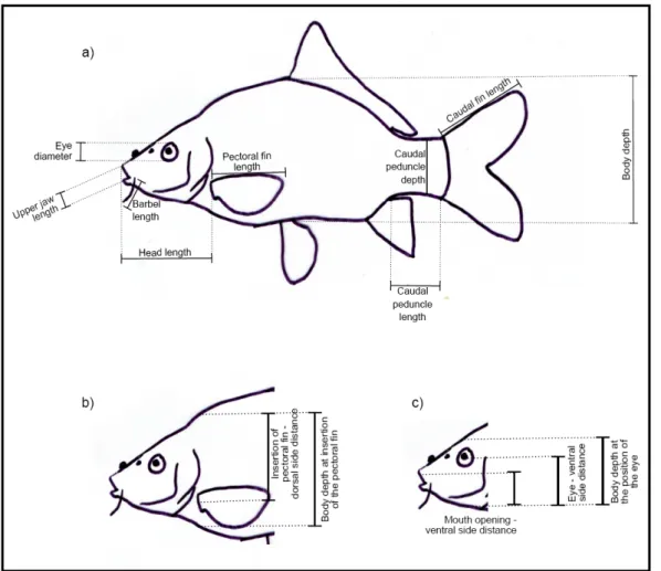
http://ddsdx.uthscsa.edu/dig/ itdesc.html. The traits, which are shown in Fig. 2.5., were equally weighed (Appendix III, table 2.1.). All fish pictures needed to measure the traits were collected from the sources listed in Appendix IV. Only pictures where the traits of interest were visible and measurable were chosen. The ideal picture showed the fish from the side taken from a 90° angle to the surface on which the fish was lying. Measurements for 26 species that also occur in Europe were taken from a study that Schleuter (pers. comm.) had previously done for Europe.

Fig. 2.5.: Picture showing the functional traits measured on the whole fish a, and on the head in detail b, c (Schleuter pers. comm.).

To make the measurements comparable among species, all measurements were standardized to the standard length of the fish, except for the number of barbels, the mouth and eye position, the two ratios - maximum body depth to caudal peduncle depth and maximum body depth to caudal peduncle length. To obtain the position of

(29)

the pectoral fin, the top body – pectoral fin distance was divided by the body depth at the pectoral fin insertion. Mouth-, pectoral fin - and eye positions were calculated by dividing both bottom head – mouth distance and bottom head – eye distance by head diameter respectively. The number of barbels and the maximum length was extracted from literature (Lee et al. 1981, Moyle 2002) and www.fishbase.org.

The significance of each trait in terms of functional expression for the animal is listed in table 2.1. The traits have been divided into two categories according to their role for the movement and behaviour of the fish (Dumay et al. 2004, Gatz 1979, Schleuter pers. comm., Sibbing et al. 2001, Webb 1987). The traits related to “habitat

and swimming ability” consist of pectoral fin length (PL), its position (PFPos), the

maximum body depth (BdD), the caudal peduncle length (CpL), and the caudal peduncle length relative to the maximum body depth (CpL/BdD), the caudal peduncle depth relative to the maximum body depth (CpD/BdD), the length of the caudal fin (CL) and the position of the eye (EP). These describe the fish’s ability to swim, turn and manoeuvre and sheds light on its habitat by speed, swimming skills and position in the water column. The group “diet and food acquisition” consists of the traits mouth position (MP), eye diameter (ED), barbel length (BarbL), head length (HL), length of the upper jaw (UJawL) and maximum body length (Lmax) and gives information about the prey size, the location of food acquisition and the detection of prey items.

To reveal intraspecific variations of the traits measured caused by the different quality of the pictures and to test the accuracy of my measurements, the coefficient of variation (CV = standard deviation/mean*100) was calculated for all trait measurements. It expresses the standard deviation in percent of the mean value. All values with a CV of more than 30 % were measured again. In case no correction was possible due to the low quality of the image (mostly of head or mouth region) the photos were excluded. Exceptions were made for some cases, where the picture collection was rather awkward and the few pictures available had to be included. In these pictures however CV is not higher than 40%.

(30)

Table 2.1.: Significance of the morphological traits for the performance of the fish grouped into their functional classes and their treatment or calculation.

Niche Axis Morphological trait Interpretation Treatment

Habitat and swimming

Ability PL Pectoral fin length Manoeuvre speed, swimming velocity Standardized by standard length

PFPos

Pectoral Fin Position Turning capacity Division of top body-pectoral fin distance

(BdpD) by body depth at pectoral fin insertion (BdDp), both

standardized

BdD

Maximum body depth

Manoeuvrability, hydrodynamics in the habitat Standardized by standard length CpL

Caudal peduncle length Swimming speed, endurance, acceleration Standardized by standard length

CpL/BdD

Caudal peduncle length relative

to max. body depth

Swimming speed Both values

stadardized by standard length

CpD/BdD

Caudal peduncle depth relative

to max. body depth

Swimming ability Both values

stadardized by standard length

CL

Caudal fin length Swimming ability Standardized by standard length

EP

Eye Position Vertical Position in the water column Division of bottom head-eye distance

(HeD) by head diameter HD Diet and food

acquisition MP Mouth position Location of food acquisition Division of bottom head-mouth distance (HmD) by head diameter (HD) ED Eye diameter Adaptation to light conditions, size of prey items

Standardized by standard length

BarbL

Number of barbels Non-visual food detection,

indicating benthic feeders

Retrieved from literature

HL

Head length Relative prey size Standardized by standard length

UJawL

Upper jaw length Relative prey size Standardized by standard length

Lmax

Maximum length Actual prey size Retrieved from literature

2.3. Calculating the Functional Diversity Indices

Since functional diversity indices (Daufresne et al. 2008, Diaz et al. 2001, Diaz et al. 2007, , Mason et al. 2003, Mason et al. 2005, Petchey et al. 2006, Schleuter et al.

(31)

accepted) are not independent of species richness, each index was calculated from actual observed values based on randomised null models of the fish communities (Gotelli et al. 1996). The 1000 null models run were then summed in one value with formula I:

SES = Obs-meanExp/sdExp (formula I)

where, SES = standardized Index, Obs = non standardized, observed value, meanExp = mean

of the randomisations, sdExp = standard deviation of the randomisations;

Each Index was calculated two times, once for the basins containing only the native species and a second time for the complete occurrence in all basins, including also non-native species. However a basin had to show at least a number of three species, the minimum needed to calculate FE and FD. The basins Santa Clara, Santa Margarita and San Louis Rey have therefore been excluded from the calculation of Indices of only native species.

2.3.1. Functional Richness (FR)

The FR Index measures how much of the niche space is actually occupied by the present species. It is obviously related positively to species richness (SR), although two communities with the same SR may show different FR. This depends on the trait distribution in the two communities. Communities with a very low FR and a high SR have uniform niche occupation among the different species, which have similar trait values. This might be the case for example after adaptive radiation of one species followed by the emergence of several subspecies with similar trait characteristics. A high FR in a community with low SR indicates that the few species present differ substantially in terms of their trait characteristics and their functional distribution in the ecosystem, thus in their niche occupation. A situation where FR is within the same range as SR occurs, when the species are randomly distributed in the niche space and different niches commanding diverse trait compositions are occupied.

Following the recommendations and instructions of Schleuter et al. (in press) the one-dimensional FRls Index was used to measure FR (formula II). FRIs is based on the variability of traits of single species instead of the community´s trait range, and is calculated as the union of all species´ trait ranges at one site, relative to the union of

(32)

species´ trait ranges at all sites together.

( )

[

]

( )

[

]

∫

∈ ∈ dx x dx x st c S s st c S s ₁ 1 U max max FRIs Functional Richness (one-dimensional) Where st

( )

x 1

is 1 if x is between min and max, else it is 0

where, s and t = notations for species and traits respectively, Sc = set of species present in the community c;

formula II

This Index is more appropriate than the other existing FR-Indices since it takes the existence of empty space within the functional trait space into account, and therefore reflects communities with uneven trait distribution much more adequate. It is further orthogonal to the FE- and FD-Indices used, indicating that the three are not correlated with each other. The increase of absolute, non standardized FR attributed to the introduction of non-native species (Fig. 3.8.) is expressed as ∆FRI and calculated according to the formula III, where FRi(Obs) is the observed Functional Richness of both native and non-native species and FRii(Obs) is the FR of only native species:

∆ FRI = FRi(Obs) - FRii(Obs) (formula III)

2.3.2. Functional Evenness (FE)

The FE Index measures how the traits are distributed within the occupied trait space. A high FE indicates that the traits are regularly distributed. A low FE indicates that traits cluster in separate clouds, and that there are unused resources or under utilised niche space. It applies to the species abundance within a niche space.

As for FR, an appropriate FE Index is used according to the recommendations and instructions of Schleuter et al. (in press). The multivariate FEm (formula IV) provided the best fit to the data. It uses the abundance- weighted Euclidian distances between all species to calculate first the minimum spanning tree (MST) that links all the species in a multidimensional trait space and then measures the regularity of the branch lengths of the MST.

(33)

FEm Functional Evenness (multi-dimensional)

( ) (

_{( ) (}

)

₎

1 1 1 1 1 1 1 , / ' / min ' ' − − − − ⎥ ⎥ ⎥ ⎦ ⎤ ⎢ ⎢ ⎢ ⎣ ⎡ −

∑

_∑

∈ ∈ c c E e c E e e e S S S A A e dist A A e dist formula IV

Where dist(e) = Euclidian distance, Ae = sum of the abundances of the endpoint species of

edge e in the minimum spanning tree, Sc = set of species present in the community c, A =

total abundance of all species;

2.3.3. Functional Divergence (FD)

Functional divergence is a measure of the variance of species´ functions and the position of their clusters in the trait space. The higher the FD values for a community the lower the competition for resources will be, since functional divergence is a measure of diversity of niche occupation. Since all available FD indices meet the requirements, it was rather unproblematic choosing an appropriate Divergence Index (Schleuter et al., in press). However, following the recommendations of Schleuter (in press), the FDQ-Index was chosen. This index is based on the Simpson index to calculate species diversity. It weighs the trait-based distances between pairs of species (dist(s,s´)) by the product of their relative abundances and is calculated according to formula V:

FDQ Functional Divergence

where, As = abundance of species, Sc = set of species present in the community, dist(s,s’) =

distance between species pairs based on mean trait values; (multivariate) s

∑ ∑

∈Scs∈Sc s s _dist _s _s A A A ' 2 ' ₍ _, _'₎ formula V

2.4. Testing for normality

To test whether data are normally distributed, a Shapiro Wilk Normality test was conducted in R with the shapiro.test() - function. This test was developed in 1965 by Samuel Shapiro and Martin Wilk to test the null hypothesis that a sample x originate from a normally distributed population. As in other tests for statistical significance the null hypothesis is rejected if the p-value is less than a chosen α-value, here 0.1,

(34)

following the recommendations of Royston (1995) and as prescribed by default in the R software. Log-transformation was used to normalize data for temperature, actual evapotranspiration, number of non-natives, number of natives, portion of cropland, degree of urbanisation, total human population and basin area. Functional divergence is very close to a normal distribution and was therefore not transformed. For the results of the single Shapiro tests see Appendix V.

2.5. Testing the 3 Hypothesis for Biological Invasion

2.5.1. Biotic Acceptance Hypothesis

To see whether data confirmed this hypothesis, I correlated the number of non-native species with temperature, actual evapotranspiration, basin area and precipitation.

2.5.2. Biotic Resistance Hypothesis

To control whether this hypothesis is applicable to the data, the number of native species and their functional diversity indices were correlated with the number of non-native species.

2.5.3. Human Activity Hypothesis

This hypothesis was tested using data on total human population in the basin areas, degree of urbanisation and extent of agricultural use, in terms of cropland cover.

2.6. Single trait distribution along the temperature gradient

To reveal the changes in the mean of single trait values per basin as a function of the addition of native species, all single traits were separated for native and non-native species and plotted against temperature. Traits were further classified according to their functional group. The function xy-plot() in the lattice package of R was used. 22 CemOA : archive ouverte d'Irstea / Cemagref

(35)

2.7. Principal Component Analysis (PCA)

Principal component analysis was invented in 1901 by Karl Pearson. It was originally not meant for ecological analysis, but it is widely applied by ecologists nowadays (Leyer et al. 2007, Ludwig et al. 1988, Manly 1994). It is a common method in multivariate statistics to explore data. The basic principle is the transformation of a number of possibly correlated variables into a smaller number of uncorrelated variables. For this purpose, the data are projected on factorial plans, which means that the data are projected on axes to maximize the variance of the projection. The data cloud itself is the projection of the data in n-dimensions, where n is the number of variables. The maximisation of represented variances is therefore not far from maximising the size of the projection of the cloud on the axis in the factorial plan. The resulting components are linear combinations of the initial variables. In fact, it is a tool to make multivariate data more manageable. PCA like other factorial analysis make it easier to visualize multivariate data, thanks to the reduction in number of dimensions (Veslot pers. comm.).

First step is the calculation of a variance-covariance matrix, which for a normed PCA corresponds to the matrix of Pearson´s linear correlation coefficient (PLCC), r. This matrix, say the correlation matrix, is a symmetric matrix that gives the PLCC for all the pairs of variables. It is possible to visualize r geometrically in a triangle, which is the basis for the graphical explanation of a PCA (Leyer 2007).

The traits are in the present case considered as vectors in the basin space and r is the scalar product divided by the product of standard deviations, which is here equal to 1 because of standardisation. If r is zero the two vectors are orthogonal, if r is 1 the two traits are parallel and in the same direction, if r is -1 they are parallel but in opposite direction. Because of prior standardisation, all vectors have by default the same length, the same point of origin and enclose an angle α. The size of α is dependent on the strength of correlation between the two vectors (Fig. 2.6.). This correlation is also named “loading”. α can be calculated following the rules of simple trigonometry due to the fact that a connection between point B on OB and S on OS encloses a right-angled triangle. The distance OS ( sr ) is therefore the adjacent leg, OB (bv) the hypotenuse and the cosine of α is sr /bv. Since bv is by default 1 due to standardisation (included as a constraint in the calculation for maximum variance),

(36)

the cosine of α is equivalent to the length of sr . The size of α thus indicates the length of , which ranges between -1 and 1, like the Pearson coefficient of correlation. sr

0 0 0

B

S

α α α

a

b

c

Fig. 2.6.: Graphical demonstration of correlation between two variables shown as vectors. Situation a indicating a strong positive correlation, b showing two orthogonal vectors indicating no correlation at

all and c showing a strong negative correlation.

A similar scenario can be created in more difficult cases with more than one variable and therefore more than one vector. The principle component analysis now tries to connect all these vectors by a common axis that maximises the sum of of all vectors. This expresses the maximum variation possible and in practice is the coordinate on the new basis vector. Since negative values appear for negative correlations, the s -values are squared. This sum is then expressed as the eigenvalue of an axis (formula V) and the sum of the eigenvalues is equal to the sum of the variables for a normed PCA (Dufour 2008).

sr sr

r

EV = OS1² + OS2² + OS3² + … Formula V

The eigenvalues are usually plotted in a barplot that indicates the decreasing importance of the axis. Most importantly, any following axis will always be orthogonal to the prior axes, which signifies that it is independent.

The PCA reduces the number of dimensions and summarizes the redundant information through few principal components. The axes with low EV can probably be interpreted as statistical noise. The choice of the relevant number of components is a difficult task and the existing rules are mostly empirical. I therefore based my decision of relevant components on an eigenvalue of more than one, which is a common method. The division of eigenvalues by the number of variables analysed gives the importance of the component in percentage of the variance it explains. Mathematically, the computation of eigenvectors (and eigenvalues) is a problem of

(37)

maximisation under constraints, which can be solved using the Lagrangian approach (Veslot pers. comm.). The expression of the lagrangian method is of the form L = V – λ * c. Where V is the variance of the projected data, λ is the unknown eigenvector and c is the constraint. The eigenvector is here normalized to one and for each orthogonal axis the prior axes are added as additional constraints. The derivation of this expression gives the maximum L and from this λ can be retrieved. It is equivalent to the variance of the coordinates of the projection of data points onto the component of a sample. For all plots, only the first and the second axis were taken into consideration, apart from the s.corcircle plots where the general representation of the single traits on the factorial plans also includes the third axes.

To conduct PCA using the dudi.pca() function in the ade4 R-package, I generated a database with the mean trait values of species occurring in the basins. Since both the mean trait value per basin and the mean trait value of all basins are projected on the same factorial plans a conjoint interpretation is possible. In fact, this ordination method is a way to graphically interpret the trait characteristics for the single basins. This method was also used to correlate the trait distribution with environmental parameters and the biological influence of non-native occurrence. This was done by the cex() command in R, which plots the size of a data point according to the value of an additional variable. An s.class plot was generated for displaying the trait distribution of basins that have non-native occurrence lower than 33% and basins in which non-native occurrence is higher than 33%. An s.class plot is basically a grouping of points according to the levels of one or more factors, here the 33% non-native occurrence. 25 CemOA : archive ouverte d'Irstea / Cemagref

(38)

0 500 1 000 km

CANADA

USA

Native Species Richness Studied basins USA SRna 0 - 10 11 - 20 21 - 30 31 - 40 CemOA : archive ouverte d'Irstea / Cemagref

(39)

0 500 1 000 km

CANADA

USA

Non-native Species Richness Studied basins

SRnn 0- 5 6- 10 11 - 15 16- 20 21- 25 26- 30 Alosa sapidissima

Ce m OA : a rc hi ve o uv ert e d'I rs te a / C e ma gr ef

(40)

CemOA

: archive

ouverte

d'Irstea

(41)

0 5 10 15 20 25 30 35 Big .Sur Che halis Stil lagu am ish Nis qual ly Sal inas San ta.M aria .Cal Bea r.riv er Wa lker Nap a San .Lui s.O bisp o Fras er Car mel San ta.M arga rita Eel San ta.In ez San .Lui s.R ey Dea th.V alle y Hum bold t Rus sian Sac ram ento Kla mat h Cos um nes San ta.C lara San .Die go Col um bia San .Joa quin Los. Ange les n ° n o n -n ati ve sp eci es CemOA : archive ouverte d'Irstea / Cemagref

(42)

0 5 10 15 20 Salve linus.fo ntinal is Lepo mis. microlo phus Notem igonu s.cry soleu cas Ameiu rus.c atus Doro soma. peten ense Ameiu rus.ne bulos us Pomo xis.a nnula ris Salm o.trutt a Pimep hales .prom elas Caras sius. auratu s Ameiu rus.m elas Ictalu rus.p uncta tus Cypri nus.c arpio Pomo xis.n igrom acul atus Micro pteru s.dol omieu Alosa .sapid issi ma Gamb usia. affinis Lepo mis.c yane llus Lepo mis.m acroch irus Micro pteru s.sal moide s Oc cu rr en ce ∆ ∆ Ce m OA : a rc hi ve o uv ert e d'I rs te a / C e ma gr ef

(43)

CemOA

: archive

ouverte

(44)

0 500 1 000 km

CANADA

USA

Studied basins 00.0.1- 0- 0.1.2 0.2- 0.3 0.3- 0.4 0.4- 0.5 ΔFRI ΔFRI Ce m OA : a rc hi ve o uv ert e d'I rs te a / C e ma gr ef

(45)

CemOA

: archive

ouverte

(46)

CemOA

: archive

ouverte

(47)

Alosa sapidissima CemOA : archive ouverte d'Irstea / Cemagref

(48)

CemOA

: archive

ouverte

(49)

CemOA

: archive

ouverte

(50)

CemOA

: archive

ouverte

(51)

3.4.1.1. Temperature [°C]

3.4.1.2. Actual Evapotranspiration [mm*a(-1)_]

3.4.1.3. Basin Area [km²]

3.4.1.4. Precipitation [mm*day(-1_)]

3.4.2.1. Number of native species

(52)

FR FE FD p-value Adjusted R² CemOA : archive ouverte d'Irstea

(53)

Adjusted R²

3.4.3.1. Total human population

Ce m OA : a rc hi ve o uv ert e d'I rs te a / C

(54)

3.4.3.2. Urbanisation

3.4.3.3. Cropland

Lampetra Anguilla

(55)

CemOA

: archive

ouverte

(56)

CemOA

: archive

ouverte

(57)

CpL.BdD 0.5 -0.7 CpL -0.8 CpD -1.0 CpD.BdD -0.8 PL -0.9 PFPos 0.9 ED -0.9 EP 0.7 MP -0.5 0.5 HL -0.9 UjawL 0.9 Lmax_cm 0.7 0.5 BarbL -0.8 CemOA : archive ouverte d'Irstea / Cemagref

(58)

CemOA

: archive

ouverte

(59)

CemOA

: archive

ouverte

(60)

CemOA

: archive

ouverte

(61)

CemOA

: archive

ouverte

(62)

4. Discussion

4.1. Non-native species and their distribution

One third of all fish occurrence data in the selected drainage basins is of non-native nature and half of the basins have at least 25% non-native species. This is in accordance with the present trend of a redistribution of species and biological invasion that is menacing biodiversity worldwide (Nentwig et al. 2007). Accordingly, Leprieur et al. (2008) found that the pacific coast of North America is one of the six global hot spots of freshwater fish invasion. The other five regions are distributed all over the world (pacific coast of South America, southern South America, western and southern Europe, central Eurasia, South Africa and Madagaskar, South Australia and New Zealand). All six regions are characterised by the highest proportion of native fish species appearing on the IUCN red lists, that indicate a high risk of extinction in the wild (Leprieur et al. 2008).

Most non-native species in pacific North America are established in the southernmost basins. The biotic acceptance hypothesis showed that the number of non-natives is positively correlated with temperature. A warm climate favours performance in general and might also promote the adaptation of generalists to a new environment. Spawning is for some fish species triggered by certain temperatures to guarantee gamete viability, growth and survival (Hokanson 1977). Besides, the overall activity level in many fish species is determined by temperature (Hokanson 1977). On the contrary, low water temperatures may lead to slow growth in some species and inhibit recruitment in others (Patton et al. 1996).

Another major factor influencing non-native success is, according to the biotic acceptance hypothesis, the basin area. Although, there was no correlation between the two variables in the present case, other studies have shown a general positive relationship between basin area and the number of non-native species (Gido et al. 1999). However again other studies suggest that basin area only has a minor effect on their numbers (Leprieur et al. 2008). Neither evapotranspiration nor precipitation, which are two further parameters suggested to play a role in the establishment of non-native species (Leprieur et al. 2008), appeared to affect the abundance of non-non-native species in the present study.