Part III
Appendices
Appendix A
Equations of fluid motion
A.1
Navier-Stokes equations
Fluid flow is characterized by a set of partial di↵erential equations, which describe the conservation of mass, momentum (Navier-Stokes equations) and energy in a compressible fluid (using Einstein’s summation):
@⇢ @t + @⇢ui @xi = 0 (A.1) @ @t⇢ui+ @ @xj ⇢uiuj = @P @xj ij + @Tij(v) @xi (A.2) @⇢E @t + @ @xj(⇢ujE) = @qi @xi + @ @xj(ui(P ij+ T (v) ij )) + ˙Q (A.3)
In Eqs. (A.1)-(A.3), E is the total energy of the fluid, u is the velocity vector, ⇢ is the fluid density, T(v) is the viscous stresses tensor, q is the heat flux and ˙Q is a heat source term (if existing). Finally, this set of equations is accompanied by the perfect gas law:
P = ⇢rT (A.4)
where r is the specific gas constant of the fluid and is equal to r = R/W , where W is the molar mass of the fluid and R is the molar gas constant equal to 8.314472 J/K/mol. The viscous stress tensor for Newtonian fluids (such as air) can be computed as:
Tij(v) = 2 3µ @uk @xk ij + µ ✓ @ui @xj + @uj @xi ◆ (A.5) where µ is the dynamic viscosity of the fluid. It is a function of the temperature, and throughout this work it follows a power law with respect to a reference viscosity and temperature: µ(T ) = µref ✓ T Tref ◆ 0.695 (A.6)
162 Chapter A : Equations of fluid motion
Finally, the formula for the heat flux q reads:
qi = @T
@xi (A.7)
In Eq. (A.7), is the heat conduction coefficient, calculated using the Prandtl number
P r (assumed constant) using = µCp
P r.
These equations describe the flow in the absolute frame of reference. If the equations are to be resolved in the relative frame of reference for rotating blades, as if an observer was sitting on the blade surface, the velocity is switches to the relative velocity for which 2 additional forces impact its evolution. These are a) the centrifugal force fv = !2R, where ! is the angular velocity, R the radius, and b) the Coriolis force fcor = 2!⇥ W , where W is the relative velocity. The relative and absolute velocities are linked through the formula V = W + U, as shown in section 1.3, with U being the rotational velocity of the blade.
Reacting flows are governed by the same equations complemented by the fact that the combustion of hydrocarbons leads to a large number of di↵erent species constantly created and consumed by chemical reactions. As a result, species conservation equations are introduced and the energy equation is modified to account for the reaction charac-teristics and forces exerted on the species [25]. For k = 1, ..., N components the species conservation equation reads:
@⇢Yk @t + @ @xj (⇢ujYk) = @ @xj Jj,k+ ˙!k (A.8)
and the energy equation reads: @⇢E @t + @ @xj(⇢ujE) = @qi @xi + @ @xj(ui(P ij+ T (v) ij )) + ˙Q (A.9)
In Eq. (A.8), Vk is the di↵usion velocity of species k, Yk is the mass fraction, Ji,k is the di↵usion flux for species k and ˙!k is the reaction rate for species k.
The heat flux is modified to take into account the flux due to the di↵usion of the species: qi = @T @xi ⇢ N X k=1 Ji,khs,k, (A.10)
where hs,kis the sensible enthalpy of species k. In Eqs. (A.10) and (A.8), Ji,k is formulated as: Ji,k = ⇢ ✓ DkWk W @Xk @xi YkVic ◆ (A.11) where Xk is the molar fraction of species k, Dk is the di↵usion coefficient of the species k and Vc
i is a correction velocity to ensure mass conservation [25]. The di↵usion coefficient of species k is calculated as:
A.2 Filtered Navier-Stokes equations 163
Dk = µ
⇢Sc,k
, (A.12)
where Sc,k is the Schmidt number of species k. Finally, the correction velocity Vic is computed as: Vic = N X k=1 DkWk W @Xk @xi . (A.13)
It is important to note that the gas constant r of the fluid is now dependent on the molar mass of the mixture W , computed as:
1 W = N X k=1 Yk Wk (A.14)
A.2
Filtered Navier-Stokes equations
LES was first introduced in 1963 by Smagorinsky [171], in an attempt to directly simulate the large eddies existing in turbulent flows while modeling those in the sub-grid scales. For compressible flows, a spatial mass-weighted Favre filtering is performed [25]:
⇢ ˜f (x, t) =
Z 1
1
⇢f (x0)G(x x0)dx0 (A.15)
where f can be any variable and G is the filter function. The overbar denotes a filtered variable while the tilde denotes the Favre filter operation ˜f = ⇢f⇢. Thus, a RANS-like decomposition f = f + f0 still exists, however f is the filtered variable and not its statistical or temporal average. It is noted that the filter function satisfies the normalization condition:
Z 1
1
G(x)dx = 1 (A.16)
Performing the filtering allows to resolve the large scales of turbulence, while cutting o↵ the smaller ones. The filter width allows also to determine the extent of the resolved scales compared to the unresolved ones. Applying the filtering to the equations of motion (assuming that the filter is homogeneous and the filtering operation commutes with the gradient) yields for the mass conservation:
@⇢
@t +
@⇢ ˜Uj
@xj = 0. (A.17)
164 Chapter A : Equations of fluid motion " @⇢ ˜Ui @t + @⇢ ˜UiUj˜ @xj # = @ @xj[P ij T (v) ij ⌧ijr], (A.18) @⇢ ˜E @t + @ @xj(⇢ ˜E ˜Uj) = @ @xj[uj(P ij ⌧ij) + qj + q r j] + Q. (A.19)
The species equation becomes: @⇢ ˜Yk @t + @ @xj ⇣ ⇢˜ujYk˜ ⌘= @ @xj ⇥ Jj,k + Jj,kr ⇤+ ˙!k. (A.20)
Equations (A.18) - (A.20) give rise to similar closure problems as in RANS, notably for the residual stress ⌧r
ij, the residual heat flux qjr and the sub-grid scale di↵usive species flux vector Jr
j,k. They are respectively defined by:
⌧ijr = ]UiUj Ui˜ Uj˜, (A.21a)
qir= ⇢⇣UiEg Ui˜ E˜⌘, (A.21b)
Ji,kr = ⇢( guiYk ui˜Yk).˜ (A.21c)
These terms represent the unresolved turbulent length scales that the mesh is in-capable to capture. This concept is illustrated in Fig. A.1, where a set of eddies is superposed to a numerical grid. The larger red eddies are the ones that can be resolved with a few cell points available per eddy diameter, while the blue ones are too small to be captured by the mesh and will be removed by the filtering operation. For a good quality LES, the mesh construction should be such to enable the resolution of the large eddies well into the inertial sublayer of the turbulent spectrum, while cutting o↵ the small scales that contain only a small part of the turbulent kinetic energy [54].
A.2.1
LES modeling
While the sub-grid scales hold a small portion of the kinetic energy (Chapman [54] sug-gests that LES should be able to resolve around 90% of the total turbulent kinetic energy), they are responsible for the dissipation of energy in the turbulent cascade. As a result, ignoring them would result very quickly in energy accumulating in the system. To rectify this, modeling is required by means of a so called Sub-Grid Scale (SGS) model, in an attempt to mimic the real behavior of the finest turbulent scales onto the resolved field. To achieve this objective, as with several RANS turbulence models, the Boussinesq ap-proximation is commonly employed. For the SGS stress, the Boussinesq apap-proximation links it to the filtered rate-of-strain. It reads for compressible flows [25]:
⌧ijr ij 3 ⌧kk= 2⌫t ✓ ˜ Sij ij 3 Skk˜ ◆ (A.22) 164
A.2 Filtered Navier-Stokes equations 165
Eddies to resolve
Sub-grid scale eddies
Figure A.1: The LES concept: large turbulent scales can be resolved by the mesh while the smaller ones have to be modeled
In Eq. (A.22) Sij = 1
2 ⇣ @Uj @xj + @Uj @xi ⌘
is the filtered rate-of-strain tensor and ⌫t is the turbulent viscosity that is to be closed. Several SGS models exist in the literature.
Below, a short description of three commonly used SGS models employed in this thesis is provided.
• Smagorinsky SGS model [171]
It is the most elementary model developed for LES. It has the advantages of being easy to implement and robust. It is often used in conjunction with wall modeling to avoid numerical instabilities. The formula for the eddy viscosity reads:
⌫⌧ = l2SS = (Cs )2 q
2SijSij (A.23)
In Eq. (A.23) lS is the Smagorinsky length scale and Cs is the Smagorinsky coeffi-cient, usually taken to be around 0.18.
• Wall Adapting Local Eddy-viscosity model (WALE) [57]
Developed by Nicoud et al [57], the WALE model aims at capturing the change of scales close to walls without using a dynamic approach, such as the one proposed by Germano [222], therefore reducing the computational cost. Contrary to the simple Smagorinsky model, WALE model disappears in cases where there is pure shear.
⌫⌧ = (Cw )2 (s d ijsdij)3/2 ( ˜SijSij)˜ 5/2+ (sd ijsdij)5/4 (A.24)
166 Chapter A : Equations of fluid motion with sd ij being: sdij = 1 2(˜g 2 ij + ˜gji2) 1 3g˜ 2 kk ij with ˜gij = @ ˜ui @xj, (A.25) • model [168]
The model, developed by Nicoud et al [168], attempts to satisfy all the above
mentioned properties P1-P3. Instead of being based on the strain rate tensor, its operator is formulated based on the singular values ( 1, 2, 3) of the velocity gradient tensor:
⌫⌧ = (C )2D with D = 3( 1 2)(2 2 3)
1
, (A.26)
where C = 1.5. It is the most recently developed of all the models employed, hence its capacity in handling more complex configurations has not been tested.
As with RANS models, SGS models are not perfect and might not follow certain uni-versal flow properties and erroneously introduce additional turbulent viscosity. Besides modeling the sub-grid scales, all SGS models should be able to follow three universal prop-erties. A primary property is that turbulence stresses are damped near the walls (they scale with y3, where y is the distance from the wall [167]), thus turbulent viscosity should follow the same behavior (named property P1). Additionally, two other desired proper-ties are that turbulent viscosity should be zero in case of pure shear and pure rotation (property P2) as well as when there is isotropic or axisymmetric contraction/expansion (property P3) [168].
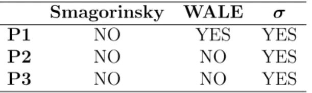
Table A.1 summarizes which of the desired properties are satisfied by the formulation of the three SGS models.
Smagorinsky WALE
P1 NO YES YES
P2 NO NO YES
P3 NO NO YES
Table A.1: Summary of the three sub-grid scale models, their constants and whether they satisfy the desired properties
The SGS contribution to the heat flux is modeled simply as: qir= t@ ˜T @xi + N X k=1 Ji,kr hs,k (A.27)
In Eq. (A.27) tis a modified heat conduction coefficient, calculated based on a constant
turbulent Prandtl number, here assumed constant and equal to P rt = 0.6, and the
turbulent viscosity as:
A.2 Filtered Navier-Stokes equations 167
t = ⌫tCp P rt
(A.28) Similarly, the SGS di↵usive species flux vector is computed as:
Ji,kr = ⇢ DktWk W @ ˜Xk @xi Yk˜ V˜ c,t i ! (A.29) where Dt k = S⌫tt c,k, with S t
c,k being the turbulent Schmidt number, here equal to 0.6 for all species.
168 Chapter A : Equations of fluid motion
Appendix B
Combustion modeling
A difficult problem is encountered in Large Eddy Simulations of premixed flames: the
thickness 0
Lof a premixed flame is generally smaller than the standard mesh size xused for LES. For this reason, the Dynamic Thickened Flame (TF) model has been developed to facilitate the resolution of flame fronts on a LES mesh. To achieve that, the flame
is thickened by multiplying the di↵usive fluxes by a thickening factor F. This flame
thickening factor is dynamically determined to have a maximum value in the flame zone and decrease to unity in non-reactive zones as:
F = 1 + (Fmax 1)S (B.1)
where S is a sensor to determine the flame position depending on the local temperature
and mass fractions and Fmax = Nc
x
0
L with Nc being the number of cells used to resolve the flame front. The necessity for a sensor becomes evident if one considers that in non reactive zones, where only mixing takes place, the molecular and thermal di↵usions will
be overestimated by a factor F if a non-dynamic approach is employed. In these zones,
the thickening factor should be corrected to go to unity.
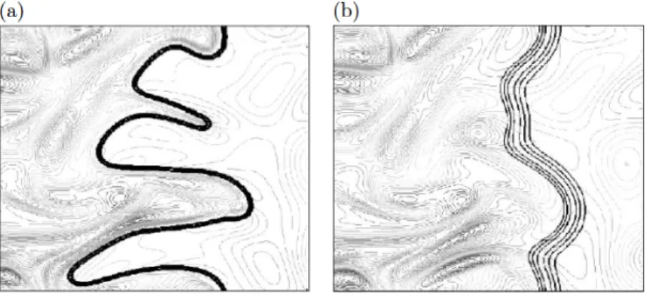
Figure B.1: Direct Numerical Simulation of flame/turbulence interactions by Angelberger
et al. [24] and Poinsot and Veynante [25]. (a) non-thickened flame and, (b) thickened flame (F = 5)
170 Chapter B : Combustion modeling
In turbulent flows, simply thickening the flame front is not enough as the interaction between turbulence and chemistry is altered: eddies smaller than 0
L do not interact with the flame any longer. As a result, the thickening of the flame reduces the ability of the vortices to wrinkle the flame front. As the flame surface is decreased, the reaction rate is underestimated (Fig. B.1). In order to correct this e↵ect, an efficiency function E has been developed from DNS results and implemented into AVBP. The formula for the efficiency function is defined as the wrinkling ratio between the non-thickened reference flame and the thickened flame and it reads:
E = ⌅( 0 L) ⌅( 1 L) = 1 + ↵ ⇣ e 0 L, u0 e S0 L ⌘u0 e S0 L 1 + ↵ ⇣ e 1 L, u0 e S0 L ⌘u0 e S0 L (B.2) In Eq. (B.2), corresponds to the integration of the e↵ective strain rate induced by the turbulent scales between the Kolmogorov dissipative scales ⌘K and the filter width
e, i.e the scales a↵ected by the flame thickening. It is formulated as: ✓ e 0 L ,u 0 e S0 L ◆ = 0.75exp 1.2 (u0 e/S 0 L)0.3 ✓ e 1 L ◆2/3 (B.3) where S0
L and 0Lare the laminar flame speed and thickness when no thickening takes
place and 1
L = F L0. The variable ↵ is a constant of the model and u0 e is the SGS
turbulent velocity that is computed using a Laplacian operator described in [219]: u0 e = c2 3x| @2 @xj@xj ✓ elmn @un @xm ◆ (B.4) The energy and species conservations equations with the combustion modeling be-come: @⇢ ˜E @t + @ @xj(⇢ ˜E ˜Uj) = @ @xj ujP ij 2µ˜ui( ˜Sij 1 3Skk ij˜ ) (B.5a) + @ @xj " CpEF µ P r @ ˜T @xj # + @ @xj " N X k=1 EF µ Sck Wk W @ ˜Xk @xi ⇢ ˜Yk( ˜V c j + ˜V c,t j ) ! ˜hs,k # +EQ F @⇢ ˜Yk @t + @ @xj ⇣ ⇢˜ujYk˜ ⌘= @ @xj " EFSckµ WkW @ ˜@xiXk ⇢ ˜Yk( ˜Vjc+ ˜Vjc,t) # (B.5b) +E ˙!k F 170
Appendix C
Theory of Dynamic Mode
Decomposition
The output of a typical numerical solver is a series of M instantaneous solutions (snap-shots), saved every user-specified timestep t (significantly larger than the timestep of the simulation). In DMD, each snapshot is treated as a vector of length N (usually the number of grid points times the flow variables to be analyzed). Memory constraints nor-mally dictate that N >> M . The data from the solutions can hence be represented by the following set of vectors:
VN1 ={v1, v2, v3, ..., vN} (C.1)
In Eq. (C.1). VN
1 has a size of N ⇥ M and can be split into two sets, each of size
N ⇥ (M 1):
VN 11 ={v1, v2, v3, ..., vN 1} (C.2a)
VN2 ={v2, v3, v4, ..., vN} (C.2b)
An unknown matrix A is introduced that transforms any snapshot vi in the data
sequence over one time step t:
Avi = vi+1 (C.3)
where A is a linear operator that can be considered an approximation to the Navier-Stokes equations. Applying the propagation matrix to the entire dataset VN 11 gives:
AVN 1
1 = VN2 (C.4)
The characteristics of the operator A can be studied through its eigenvectors n and eigenvalues n, which provide mode structures and frequencies respectively. However, the matrix A is either unknown or too large and a lower dimension approximation is usually looked for.
To do so, ↵ the number of snapshots M is large enough, the solution vectors become linearly dependent leading to:
172 Chapter C : Theory of Dynamic Mode Decomposition
vN =X
i<M
↵ivi+ eN (C.5)
where eN is the residual that tends to 0 as the number of snapshots M is increasing.
Using Eq. (C.5) and introducing a companion matrix S of size (M 1)⇥ (M 1)
and of the form:
S = 0 B B B B B @ 0 0 · · · 0 ↵1 1 0 · · · 0 ↵2 0 1 · · · 0 ↵3 ... ... ... ... 1 0 · · · 1 ↵M 1 1 C C C C C A (C.6) we can write: AVN 1 1 = V2N = VN 11 S (C.7)
Equation (C.7) indicates that the modes of A, of size (N 1)⇥ (N 1), can be looked for in the reduced matrix S. There are several formulations for the S matrix in the
literature, for example by expanding VN 11 via a Singular Value Decomposition (SVD)
[188] or a QR-decomposition [223]. In this work, the variant proposed by [224] is used. In this approach, the operator S is reformulated using Eq. (C.7):
S = (VN 11 ) 1VN2 (C.8)
First, introducing the SVD, one can write:
VN 11 = U ⌃WH (C.9)
where U and W are unitary matrices and ⌃ is diagonal. The superscript H indicates the
conjugate transpose of the matrix.
Then, the inverse of VN 11 is computed using a Moore-Penrose pseudo inversion [225] as:
(VN 11 ) 1 = W ⌃ 1UH (C.10)
From Eq. (C.9), U can be straightforwardly computed: U = VN 11 W ⌃ 1. Introducing it in Eq. (C.10) and replacing the whole expression in Eq. (C.8) the companion matrix can be computes as:
S = W ⌃ 1⌃ 1WH(VN 11 )HVN2 (C.11)
Considering the diagonalization:
173
(VN 11 )HVN 11 = W ⌃2WH (C.12)
the matrices W and ⌃ can be also computed from an eigenvalue decomposition of (VN 11 )HVN 1
1 .
The last step is to solve the eigenvalue problem Ssn = µnsn where sn and µn are the eigenvectors and eigenvalues of S. Note that the eigenvectors n of the matrix A, which correspond to the DMD modes, are simply the projection of sn onto the snapshot basis:
n = VN 11 sn (C.13)
The associated complex angular frequency of the modes follows:
!n= ln(sn)
t (C.14)
Finally, the global amplitude of each dynamic mode is defined simply as its L2 norm, || n||L2 =
p
174 Chapter C : Theory of Dynamic Mode Decomposition
Appendix D
MISCOG method - Journal of
Computational Physics
Journal of Computational Physics 274 (2014) 333–355 Contents lists available atScienceDirect
Journal
of
Computational
Physics
www.elsevier.com/locate/jcpAn
overset
grid
method
for
large
eddy
simulation
of turbomachinery
stages
Gaofeng Wanga,b,∗, Florent Duchainea, Dimitrios Papadogiannisa,
Ignacio Durana, Stéphane Moreaub, Laurent Y.M. Gicquela
aCFDteamCERFACS,42avenueGaspardCoriolis,31057ToulouseCedex1,France bUniversitédeSherbrooke,Sherbrooke,QCJ1K2R1,Canada
a r t i c l e i n f o a b s t r a c t
Articlehistory:
Received19October2013
Receivedinrevisedform25April2014 Accepted4June2014
Availableonline11June2014 Keywords:
Largeeddysimulation Turbomachinery Rotor–statorinteractions Oversetgrids
A coupling method based on the overset grid approach has been successfully developed to couple multi-copies of a massively-parallel unstructured compressible LES solver AVBP for turbomachinery applications. As proper LES predictions require minimizing artificial dissipation as well as dispersion of turbulent structures, the numerical treatment of the moving interface between stationary and rotating components has been thoroughly tested on cases involving acoustical wave propagation, vortex propagation through a translating interface and a cylinder wake through a rotating interface. Convergence and stability of the coupled schemes show that a minimum number of overlapping points are required for a given scheme. The current accuracy limitation is locally given by the interpolation scheme at the interface, but with a limited and localized error. For rotor–stator type applications, the moving interface only introduces a spurious weak tone at the rotational frequency provided the latter is correctly sampled. The approach has then been applied to the QinetiQ MT1 high-pressure transonic experimental turbine to illustrate the potential of rotor/stator LES in complex, high Reynolds-number industrial turbomachinery configurations. Both wave propagation and generation are considered. Mean LES statistics agree well with experimental data and bring improvement over previous RANS or URANS results.
2014 Elsevier Inc. All rights reserved.
1. Introduction
Computational Fluid Dynamics (CFD) hasbeen developed over thepast few decades and hasbeen intensively used as adesign toolofgasturbines forpropulsionor powergenerationsystems.Because ofincreasingmarketand environmental constraintsthattargethighefficiency,highpowertoweightratio,lownoiseandhighreliability,currentandnextgeneration of gasturbine engines will require improvedCFD tools. Indeed to contributeefficiently to ourunderstanding and thereby produce better engines, unsteady physical and chemical phenomena that take place in these engines need to be better apprehended.This inthelong termwillhave tobeaddressed foreachsub-component, butalso inafullyintegrated way:
i.e. simulatingatonce the compressor, thecombustor and theturbine [1]. Inthespecific context ofCFD,Large Eddy Sim-ulation(LES) [2]isa goodcandidate andhasalready been used tosimulate thecombustorof gasturbines[3,4]and some specific isolated parts of turbomachinery applications [5–13], but few applications are today available in turbomachinery stages [14–17]. Infact, CFD for turbomachinery still remainsa challenge because ofthe highReynoldsand Mach-number
* Correspondingauthorat:CFDteamCERFACS,42avenueGaspardCoriolis,31057ToulouseCedex1,France. E-mailaddress:[email protected](G. Wang).
http://dx.doi.org/10.1016/j.jcp.2014.06.006
334 G. Wang et al. / Journal of Computational Physics 274 (2014) 333–355
flows, theimportanceofseveral lossmechanisms that greatlyimpacttheoperatingcondition andefficiencyofthese com-ponentsaswellasmixing effectsbetweenhotstreamfromthecombustionchamberandfresh coolinggases, multi-species flows, rotation and technological effects. Current industrial turbomachinery simulations usually involve Reynolds-Averaged Navier–Stokes (RANS)orUnsteadyRANS (URANS)equations, whichrelyon turbulence models[18,19]to predictthemean flowfieldsintheseelements.Fortheknownrotor/statorinteractions,URANSisnecessarytocapturetheunsteady determin-isticinteractionsthatarepresentintheseconfigurations[20].TodaythecomputationalcostofRANSorURANSisacceptable forengineeringapplicationsand explaintheirdailyuseinrealapplications.Howeversuchtoolsshowlimitswheneverused fortestingoff-designpointcomputations[14]orevenatdesignconditionswhentransitiontoturbulenceorsecondaryflows playmajorroles.ThemodelingneededwithRANSorURANSlimitsengineersfromfurtherefficientlyimprovingthedevices andexpensivetestbenchingsofmultipleconceptsarestillmandatorytoday.
Withthe rapiddevelopment ofHighPerformanceComputing (HPC)[21], recentefforts havebeen madeon the predic-tionofthecomplexturbulentflowsaroundisolatedpartswithhigh-fidelityfullyunsteadyLES(seereviewbyTucker [22]). Although much more computationally intensive than RANS, LES can alleviate the modeling efforts by explicitly resolving the temporal and spatial evolutions of the large flowstructures while filtering out the smaller ones [23,24]. Preliminary demonstrations show that LES can resolve flows with transitions, separations [5,6,13] and thereby improve heat transfer predictions on structured or unstructured meshes [8,10,12]. Tip-clearance flow predictions [7] have also been addressed successfully withLES. McMullanand Page[14]have demonstrated that LES canpredict surface pressureon theMonterey cascadewithasufficientlyrefinedmesh. Algorithmicdevelopmentscomplementedbyhighperformance massivelyparallel machines allow todayto have LES solvers capable of handling 21 billions unstructured tetrahedral cells with a very rea-sonable speed-up [25] making useof up to one million cores at once [26,27]. Following the analysis of Tucker [28], this capability seemsto beapproaching LES requirementsof most gasturbines inaircraft applications. The application to real machinesiscurrentlybeinginvestigatedandthreeconfigurationsofcompressorstages[14,16,17]andonetransonicturbine stage[15,29]havealreadybeenreported:ascaledlaststageoftheCranfieldBBRcompressorwithaReynoldsnumberbased on thestatormidspanchord of Re=180,000,theCambridgeaxialcompressor (Re=350,000),theCME2axialcompressor
(Re=500,000) and the MT1 axial turbine (Re=2,600,000).Even inthese first LES predictions of compressor or turbine
stages, numerical challenges are still present. First, the high computational costs relate to the complexity of these flows with high Reynolds numbers Re∼O(105−7), which impose large grids. Secondly, the modeling difficulty comes from an
adequate resolutionor modelingofthe wall flowphysicssinceit mayhave adramaticimpacton themain blade-channel flow and vice-versa. Thirdly, current LES codes require high spatial and temporal accuracy [30] that may not survive at therotating interfacestoyield adequateand relevant unsteadypredictionsofcomponentinteractions. Indeedthe numeri-caltreatmentofarotatinginterfacewillimpacttheoveralldiscretization-schemequalityandproperties.Typically,resolved vortical,acousticandentropywavesshouldtravelwiththeflowandthereforecrosstheinterfacewithoutbeingsignificantly alteredbythenumericaltreatment topreservetheLESnatureofthesolverinthisregion.1
Thelast pointis crucialfor turbomachinery stagesimulations and israrelydiscussed orvalidated inreported LES [29]. In an attempt to provide validation of the interface treatment for LES of turbomachinery, a coupling interface based on oversetgridsispresentlyproposedand studiedwithspecificemphasisontheresultingschemeproperties.Theoversetgrid methodhasbeen proposedand developed for instancebyVolkov [31],Magnusand Yoshihara [32], Starius [33], Attaand Vadyak[34],Beneket.al.[35,36],Berger [37],Henshawand Chesshire[38,39].Ithasrecentlybeen studiedand appliedfor Computational AeroAcoustics (CAA) [40–42], coupling CFD/CAA [43], conjugate heat transfer problems [44], moving body applications [45–49] or to handle complex geometries [8,50] with very high accuracy [51,52]. It has also been used in RANS of external and turbomachinery flows where it is commonly known as the Chimera method [35] and reported as providing an equivalentaccuracy asthe sliding mesh method [53]. In thespecific RANS context where fieldsare smooth and independentof time, conservation is sufficient for the rotor/stator interface since the turbulence is fully modeled or describedbysomeextraconservation equationstowards thesteady statesolutionoftheproblem.Numerical requirements of RANS are hence limited to the interpolation scheme at the interface meshes that needs to be conservative, which is usually obtained by taking first-order area-based interpolation within the sliding mesh [54]. For LES, most of the flow structuresareresolvedso flowfieldsaretimedependentand containalargerangeofwavelengths coveringallthescales from the geometry upto thefinest local grid resolution. To preserve thequality of such simulations all this information shouldbetransferredthroughtheinterfacewithaslessinfluenceaspossibletomaintainflowcoherence,evolutionaswell asthenumericalpropertiesofthescheme.Theprimaryobjectiveisthus toavoiddissipatingordispersingthesignalwithin theoriginal context ofthe numericalscheme used awayfrom thisboundary. Tomeet suchrequirements,the oversetgrid methodisofinterestasincreasingitsaccuracyisstraightforward forstructuredmeshes[8,40,41,43,51,52,55–58],though it may lead tosome complexity in thegeneration ofthese overlapping regions [59]. Oversetunstructuredmeshes havealso beendeveloped inthepastdecade[60–64] andarerecentlybeingconsideredforahigh-orderinterfacetreatment [42,65].
Inthefollowing,theoverlappingmovinginterfaceisimplementedbasedonadomaindecompositionapproach[66]with an unstructured compressible high-performance parallel LES solver. The resulting strategy is hereafter called MISCOG for MultiInstanceSolverCoupledthroughOverlappingGrids.Thedetailsofthecouplingand associatednumericalfeaturesare
G. Wang et al. / Journal of Computational Physics 274 (2014) 333–355 335
given in Section 2. Convergence and numerical errors of the proposed method are thenchecked on canonical caseswith static or moving coupling interfaces in Section 3. A specific attention is brought to the dispersive and dissipative errors introducedbytheinterfacetreatment.Propagation ofacousticand vorticalwaves(anisentropicvortex)arefirstconsidered andthetranslatinginterfaceisintroduced.Therotatinginterfaceisthentestedonarotatingcylinder.Finallytwoexamples of the developed methodology for wave propagation and generation in an actual turbine, involving both translating and rotatinginterfaces,are presentedinSection 4.Thenew LEStool isappliedto theQinetiQMT1 highpressureturbine [67], whichhasbothhighReynoldsand Machnumberstypicalofmodernturboengines.
2. Numericalmethodandimplementation
The objective of the present section is to provide a description of the numerical methods retained for the treatment of the rotor/stator interface problem using the overset grid method. First, governing equations, numerical schemes and formalismspresentintheCFDcodeareexposedfollowedbythepresentationofthenumericalapproachintroducedtodeal withtheexchangeofinformationattheinterfacebelongingtothefixedandrotatingdomains.
2.1. Governingequations
ThefilteredLESunsteadycompressibleNavier–Stokesequationsthatdescribethespatiallyfilteredmass,momentumand energy(ρ,ρU,ρE)conservations, canbewritteninthefollowingconservativeform:
∂W
∂t + ∇ ·F=0, (1)
where W isthevectorcontainingtheconservativevariables(ρ,ρU,ρE)T and F = (F,G,H)T istheflux tensor.For
conve-nience,thisfluxisusuallydividedintotwocomponents:
F=FC(W)+FV(W,∇W), (2)
whereFC istheconvectiveflux dependingon W andFV istheviscous fluxdependingonbothW anditsgradients∇W.
The contributions ofSub-Grid Scale (SGS)turbulence models areincluded inthe viscous flux through theaddition of the so calledturbulent viscosity νt [18,24]. Forsimplicity,thepresent workrelieson thestandardSmagorinskySGS modelfor whichtheturbulentviscosityismodeledby
νt= (CS$g)2 !
2S˜ijS˜ij, (3)
where ˜Sij denotes the resolved rate-of-strain tensor, CS denotes model constant and $g denotes the characteristic filter
length,usuallycorrespondingtothelocalmeshcellsize[68].
2.2. Numericalschemes
The governing equations are solved by the unstructured compressible LES solver, AVBP in which several numerical schemesare available[27,69]. Only two ofthoseare presently considered.First, theLax–Wendroff scheme(LW) isa 2nd-order finite volume scheme in time and space, which corresponds to theaccuracy of most commercial codes as well as most ofthe turbomachinery CFD tools availabletoday [70].Secondly, thetwo-step Taylor–Galerkin finiteelement scheme TTG4A (4th-order in timeand 3rd-orderin space) provides improvedLES quality on unstructuredgrids [71].All schemes are expressed in the cell-vertex numerical discretization approach, for its compactness and effectiveness on parallel HPC. Thecell-basedresiduals,i.e.thespatiallydependenttermsoftheequationsoneachcontrolvolumeΩj,arethencalculated
byintegratingthefluxesoverthecellas:
RΩj= 1 VΩj " ∂Ωj F·n dS, (4)
where VΩj isthecellvolumeand∂Ωj itsboundarywithnormalvectorn.Sincetheintegrationisobtainedaroundavertex,
adistributedversionofthesecell-basedresidualsRk isconstructedviadistributionmatrices.OnecanhenceexpressEq.(1)
intothesemi-discretescheme
dWk dt = Rk= − 1 Vk # j|k∈Ωj DkΩjVΩjRΩj, (5)
where Vk is acontrol volume associated with anode k and DkΩj is thedistribution matrix that weights thecell residual
fromthecellcenter Ωj tonodek[72,73].
Instatic(withstationarymeshelement)parallelcomputations,thecomputationaldomainisdividedintoseveral individ-ualvertices-sharedpartitioneddomainseachofwhichisattributedtooneprocessorusingDomainDecompositionMethods
336 G. Wang et al. / Journal of Computational Physics 274 (2014) 333–355
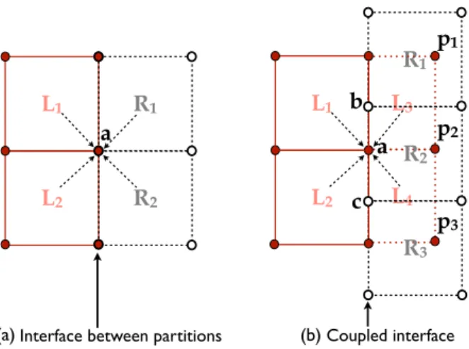
Fig. 1. (a)DDMforcell-vertexschemesusedinparallelcomputationsand(b)theproposedmethodforrotor/statorinterface.L1,2,3,4(composedof:solid lines–edgesandfilledsymbolsforthevertices)andR1,2,3(composedof:dashedlines–edgesandopensymbolsforvertices)denotethecellsontheleft andrightsidesofapartitioneddomain,respectively. Inthecaseofamovingfluidboundary,pointsa ofdomainL andpointsb,c ofdomainR arethe verticestobecoupledattheinterface.Pointsp1,2,3andL3,4areadditionalverticesinvolvedinthecouplingwhentheoverlappingmethodisintroduced.
(DDM)[66].Fig. 1(a) illustratestheconventionalDDMstaticcouplingprocessforacell-vertexscheme.Thecells(L1,2,R1,2)
aregroupedintotwo domainsrespectively denotedbyL andR andcontributetothecommonnodea cell residual.Indeed incell-vertexschemes,thecell-based residualsarecomputedlocally(i.e. for allindividualcells,L1,2,R1,2)and scatteredto
thebelongingvertices. Vertexa that islocatedatthe interfacethereforeneeds allthecontributionsfrom theneighboring partitions for thenodal residual to be evaluated following Eq. (5). In conventional approachesof static massively parallel codes,thisissimply donethroughnetworkcommunications.
2.3. Oversetmethodforrotor/statorcomputations
Theproblemfor therotor/stator couplingissimilar totheDDMproblem describedaboveexcept that thetwodomains
L and R are moving (translatingor rotating)relativelyto eachother. Non-conformalvertices(shown inFig. 1b) are hence presentatagiveninstantandalongtheinterface.Additionalevaluationsateveryiterationarethereforeneededifcompared withstaticDDM.Numerically,severalcouplingmethodsarepossibleforsuchproblems,allofwhichintroducethenotionof interpolation forinformation reconstructionaround oron theinterface. Intheimplementation, Lagrange interpolatorscan beusedforexchangingvariablesfollowing:
Lf = nsh
#
i=1
f(qi) φi, (6)
where f is a function approximated by Lagrange polynomial elements and f(qi) are the function values at the vertices
qi;nsh is the number of degrees of freedom of the element and φi are its shape functions. For nodes in an element or
on a surface, the interpolationcoefficients are calculated basedon theshape functions usingthe local coordinates ofthe elements. In the current study, simple linear shape functions, i.e. barycentric interpolation or bilinear interpolations are used inagreementwithP1 (triangularin2D andtetrahedralin3D) and Q1 (quadin2D andhexahedralin3D) elements,
implyinganorder2 fortheseoperations.
Rotor/stator interface treatment may be introduced at various steps of the numerical scheme. Coupling fluxes before computing thecell-based residuals ofEq. (4) hasthebenefit ofinvolvingonly the interfacenodes limitingthenumberof unknownsand potentialmanipulations.Withinsuchacontext,thecomputedfluxesshouldbeinterpolatedon the2D cou-pledinterfacefora3D computationasperformedinthetraditionalslidingmeshapproachforexample [54].Analternative istocouple nodalresiduals.Inthisapproach,eachnodalresidual RL
a,RbR and RRc arecalculated bycounting the
contribu-tionsofallsub-domainlocalcellsusingEq.(5)first.Thecontributionsofeachmissingdomain(i.e.:R2residualcontribution
tonodea for example)arethenestimatedbyintroducinganadditiveinterpolationLtoobtainthevertexa residualatthe interfaceforexample,
Ra= RaL+ L$RRb,RRc%. (7)
Withthisapproach,thedifficultycomesfromtherotationtermsaddedinthetransportequationsofthemovingdomain that are not compliant with the static part of theconfiguration. As a result such a schemewas found to be unstable in the case of a rotating domain coupled to a static domain if using simple linear interpolation schemes. The last solution, retained inthefollowing,consistsinreconstructingtheresiduals usinganoversetgrid methodthatdirectly exchangesthe multi-domainconservativevariablesbyinterpolation.As showninFig. 1(b),oversetgridsisintroducedrelyingonextended domainsL bytwoL3,4ormoreghostcellsinthenormal directionoftheinterfacesothatthenodalresidualofvertexa can
G. Wang et al. / Journal of Computational Physics 274 (2014) 333–355 337
Fig. 2. Communication framework of coupling rotor/stator interface.
conservative variableswithin theoverlap region to evaluate theright-hand side of Eq. (4).Note finallythat cells L3,4 are
geometrically overlapped withthedomain R with pointslocatedin cellsR1,2,3.In themoregeneric cases,theextent and
topology of the duplicated cells will not coincide. The unknown conservative variables of the overset vertices p1,2,3 are
henceapproximatedthrough aninterpolationfromtheinformationofcellsR1,2,3.Thesameprocedureisused tocompute
the nodal residuals of b,c in domain R that is also extended onto mesh L by two or more cells, since it is a two-way
coupling. This third approach is selected here asit is easily implemented externally from any base CFD code and yields high-orderaccuracyifused inconjunctionwithhighorderinterpolation[41,43,51,52,58,74].
Interms ofmethodology and overall strategy,theexternal code coupling ispreferred over an internal implementation to extendtheavailableLES solverso thatit candealwith rotor/statorsimulations. Hencetwo ormorecopiesof thesame LESsolver(namelyAVBP)eachwithitsowncomputationaldomainandstaticDDMalgorithmexecutingagivenpartitioning withagiventarget numberofprocesses,arecoupledthroughtheparallelcouplerOpenPALM[75].Thedetailed implemen-tationofsuchcouplingincludes:(1) findtheenclosedcell;(2) calculatethelocalcoordinates inthecell;(3) calculate the
interpolationcoefficientsusingashapefunction;(4)calculatetheinterpolatedvalueusingEq.(6).Thecurrent
implementa-tion[75]iscompatiblewiththeCGNSinterpolationtool [76]andisexternaltotheCFDcode.Finally,notethatahighorder interpolation isviable for unstructuredmeshes byintroducing high ordershape functions [77], but with some significant additionaleffortsinimplementingtheproperstencilsefficiently.
Fig. 2 shows a typical communication framework for a rotor/stator coupling approach using the MISCOG method de-scribed above. For this case, the whole flow domain should initially be divided into static (AVBP01) and rotating parts (AVBP02). For rotating parts, the code uses the moving-mesh approach in the absolute frame of reference while the re-mainingunitsimulatestheflowinthestationarypartinthesamecoordinatesystem[78].Theinterfacesbetweenthetwo units involving rotating and non-rotating parts are coupled with the overset grids by interpolating and then exchanging the conservativevariables wherever needed and asdescribed above. To do so, anefficient distributed searchalgorithm is implemented in the coupler OpenPALM to locate the points in parallel partitioned mesh blocks. This coupling algorithm will thenupdate at eachtime step the information and carry the interpolation from one sub-MPI world to the next and vice-versa. Issues of numerical stabilityof thecoupled solution and the convergence of thiscoupled problem aredirectly linkedtothesizeoftheoverlappedregionandthestencilofthenumericalschemesselected[79].
3. Numericalanalysisofthecouplingapproach
Prior to the application of the proposed solution to a high fidelityLES ofrotor/stator problem, three validation cases areconductedfocusingonacousticalwavepropagation(1D),convectionofaninviscid orviscous vortex(2D),androtating boundaries(2D).Eachcaseiscomputedtwice:thefirstevaluationisusedtoyieldthebenchmarksolutionusingone stan-dardAVBPprocedure runningon onemeshwhilethesecond computationuses twonon-conformal overlappingmeshes to evaluatetheMISCOGstrategy.Theprimaryobjectiveistoqualifyandquantifyerrorsintroducedbythecoupling approach.
3.1. Acousticswavetravelinginastaticcoupledsimulation
AnaccuratecompressibleLESshouldfirsttransportacousticwavesproperly.Thefirstvalidationcaseisthereforethe sim-pleproblemofa1D propagatingacousticwave(Eulerequation)inadomainwhoseboundaryconditionsarenon-reflective and theacoustic signal covers the entirecomputational domain. Fig. 3 illustrates theconfiguration for thereference and coupled simulations. In the latter, two overlapping 1D meshes are computationallycommunicating usingMISCOG. In the
338 G. Wang et al. / Journal of Computational Physics 274 (2014) 333–355
Fig. 3. 1D acousticwavepropagationsimulatedbytwoapproaches:(a)thestand-alonesolverand(b)theequivalentcoupledapproach.Thetotallengthof thecomputationaldomainisLandthecellsizeis $x.
Fig. 4. Inletwavesignal(P0)andsignalsatthedownstreamprobeforthestandardsimulation(P1)andthecoupledsimulation(P2)asafunctionoftime
tnormalizedbytheperiodT (meshresolutionof$x/λ=0.125 andLWscheme).DefinitionsofthegainfactorFandphase-shiftτ.
overlapped region, the meshes arenon-coincident and thevertices fromone mesh arelocated atthecenter ofthe corre-spondingcellintheother mesh.Theconservativevariablesover several layersofnodeson eachside arecoupledand will beupdatedbasedontheinterpolatedvaluesoftheothermeshateachtimestep.
Theincomingacousticwaveisimposedattheleftsideboundaryofthedomain(Fig. 3)usingtheInletWaveModulation (IWM)approach[80],whichisequivalenttomodulatingthetargetvelocityattheinlet as:
uinlet=U0+ P
A
ρ0c0sin(2πf t). (8)
The amplitude of the pressure perturbation is PA =100 Pa. The temporal frequency is f =1000 Hz. A zero mean flow
velocityisset(U0=0),andthedensityρ0=1.172 kg/m3andsoundspeedc0=347.469 m/s ofthemeanflowcorrespond
to atmospheric conditions. Navier–Stokes Characteristic Boundary Conditions (NSCBC) are used at both inlet and outlet boundaries toprevent wave reflections [81]. Thetotal length L of thecomputationaldomainischosen to be10 timesthe selected wave length,λ=c0/f, whichis thendiscretizedbydifferent meshresolutions, $x∈ [λ/40,λ/4].To focuson the
spatialdiscretizationerror,thetimestepsofallcasesaresettoaverysmallphysicalvalue$t=6 ms,whichcorrespondsto
aCourant–Friedrichs–Lewy(CFL)numberof0.2forthefinestmesh($x= λ/40)and0.02forthecoarsestmesh($x= λ/4).
Thetwonumericalschemes(LWandTTG4A)presentedabovearetestedhere.
Fig. 4 shows the temporal evolutions of this flowsolution obtained with LW. The inlet wave signal (P0) is compared
with the outlet probed signal for the two different approaches (P1 for the standalone computation and P2 for the
cou-pledone). Only two wave periods oftheinput signals are taken for amesh resolution $x= λ/8. In theexactsolution to
sucha problemthe sinewave shouldbepreservedand only a delay ofτex=L/c, where c standsfor thespeed of sound,
should be present at all frequencies. A gain factor F and a phase-difference τ between inlet and outlet signals are in-troduced for all simulations to assess the differences with this exact solution. The results of the standalone simulations then provide the dissipative and dispersive properties of the selected scheme. When comparing with the results of the coupledsimulations, theadditionalcontributionofthecouplingschemeandparticularlytheeffectoftheinterpolationcan beassessed. Fig. 5quantifiesbotherrors illustratedin Fig. 4.In Fig. 5(a), forlargenumbers ofpointsper wave-length, all schemesshow asmalllevel ofdissipation:thegainfactorapproachesunityinallcasesas$x/λdecreases confirming the
convergence of the discretized system (with or without interpolation). It shows that dissipation increases asthe number of pointsper wave-length decreases, making F almost vanishing when themesh resolution is poor: $x/λ=0.16 for LW
and $x/λ=0.25 forTTG4A stressing thesuperiority oftheTaylor–Galerkin schemes forcompressibleLES [30,72].Several
coupled computations with varying numbers of overlapping points No are also shown in Fig. 5(a) (No=1,4,5), to find
G. Wang et al. / Journal of Computational Physics 274 (2014) 333–355 339
Fig. 5. The gain factor F (a) and phase-shiftτ (b) errors for both standard and coupled simulations.
theoreticaland numericalanalyses[79].Usingoneorfouroverlappednodesalsoyieldsverysimilarresults.ForTTG4A,four overlapping nodesareneeded tocoverthefullstencil attheinterface. Asshown inFig. 5(a)adding afifth pointoneither side of the overlapped interface does not improve the gain factorcurve, since itdoes not appear in thestencil. Fig. 5(b) shows the phase errors for standard and coupled simulations. The curves indicate that interpolation does impact the re-sultsmainlyatverypoorlyresolvedscales.Alltheseresultsareconsistentwithconventionalanalysisofnumericalschemes designed forLESand confirmthat theproposedrotor/stator interfacetreatment meetsLESrequirements providedthatthe uncoupled discretization schemeis of highorder to minimize numerical dispersion and dissipation. This desired resultis howeverobtainedonlyif usedwithasufficientnumberofoverlappingpoints.Resultsalsoconfirmthat theinterface treat-mentcomeswithanincreaseddissipationatallresolutions. Increaseddispersionappearsmainlyfor poorlyresolvedwave lengths.
3.2. Inviscidvortextravelinginastaticandmovingcoupledsimulation
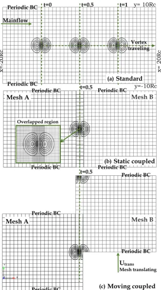
AccuratecompressibleLESalsoreliesonthemodelandsolverabilitytoresolveandtransportvortices withinacomplex geometry. The second validation case is specifically chosen to address the ability of the proposed solution to resolve a 2D vortextraveling through theoverlapped interface usingEuler equations. The numerical setupsare given inFig. 6.The standard and reference case(Fig. 6(a)) has asinglemesh composedof 2Nx×Nx quad cellsof size $x=20Rc/Nx, where
Rc is theradius of thevortex, coveringarectangular (x,y) domainof dimensions[−20Rc,+20Rc]× [−10Rc,+10Rc]. For
the coupled cases, two computational domains are provided in Figs. 6(b) and (c), and consist of two rectangular boxes with an overlapped region for which No points are present on each side of the interface. The first box covers a domain
of [−20Rc,No$x]× [−10Rc,+10Rc] and is meshed with (Nx+No)×Nx quad cells(indicated as MeshA in Fig. 6). The
secondboxcovers [−No$x+ $x/2,+20Rc]× [−10Rc,+10Rc]andhas(Nx+No)× (Nx+1)quadcells(indicatedas Mesh
B inFig. 6).Similarlyto thefirsttest case,theoverlapped vertices arelocatedatthecenter ofthequadcellsof theother mesh.Twotypesofcoupled simulationsareconducted:(1) astaticcoupling;(2) acouplingwithatranslatinginterfacein
whichthesecondcoupledmeshisperiodicallytranslatingintheverticaldirectioninFig. 6,ataconstantspeedof100,200 and 300 m/s(typicalrotatingspeedsofrelevantturbomachinery applications).NSCBCareusedagainatbothinletatoutlet boundaries to avoid wavereflections. To prevent spuriouseffects from thedomainboundaries, alllateral surfaces arealso settobeperiodic.
An initial isotropic vortex [30,81,82] is imposed on a uniform mean flow going from left to right. It is based on the streamfunction
Ψ (x,y)= Γe−r2/2R2c, (9)
whereΓ isthevortex strengthandr=&(x−xc)2+ (y−yc)2 thegeometricdistancetothevortex center(xc,yc),initially
locatedatxc= −10Rc and yc=0. Rc controlsthesizeofthevortex.Theresulting velocityandpressurefieldssimply read
u=U0+∂Ψ ∂y=U0− Γ R2 c (y−yc)e−r 2/2R2 c, v= −∂Ψ ∂x= Γ R2 c (x−xc)e−r 2/2R2 c, P =P0−ρΓ 2 2R2 c e−r2/R2 c, (10)
where P0 and U0 stand for the reference background pressure field and flowvelocity respectively. For the present
sim-ulations the different parameters are Rc =0.01556 m, P0=101,300 Pa, ρ=1.172 kg/m3 and a constant uniform flow
U0=100 m/s. Three levels of vortex strength Γ =0.036,0.1 and 0.5 m2/s are chosen leading to velocity fluctuations
u'max=v'
max=1.4,3.9 and 19.4 m/s and pressurefluctuations P'max=3.1,24.1 and 601.8 Pa respectively. The timesteps
are chosen toyield CFL=0.07 to minimize temporal effects. Additionalsimulations are obtained for CFL=0.7 as
recom-mendedforTTG4A[73].
Only predictionsfor CFL=0.07 are shown in Fig. 6for the threesimulation setups.In Fig. 6(a), theinitial vortex
340 G. Wang et al. / Journal of Computational Physics 274 (2014) 333–355
Fig. 6. Schematicofstandardandcoupledsimulationsofvortextraveling:(a)Standardcase;(b)Staticcoupledcase; (c)Movingcoupledcase:similarmesh sizesasthepreviouscoupledcase,exceptthatmeshBistranslatingatspeedofutrans=100, 200or 300 m/s.Themeshsizeis $x=Rc/4 withNx=80 andNo=4 (onlyone-fourthofgridpointsareshown).Theinviscidvortex(withradiusRc),shownbyisolinesoflateralvelocity,isinitializedattimet=0 andistraveling fromlefttorightandpassingthroughtheinterface(t=0.5).Timetisnormalizedbythevortexconvectiontimeovertraveldistance, 20Rc/U0.
standalonesetup.InFigs. 6(b)and (c)forthestatic andmovingmeshrespectively,thevortexhasreachedthecenterofthe couplinginterface.As evidencedbytheisolines,thevortexiswellpreservedinthecoupledcasesevenwhenitcrossesthe couplinginterfaces.
Numericalconvergenceoftheproposedcoupledstrategyisthenaddressedondifferentmeshresolutions(Nx from20to
200),usingboththeLW and TTG4A schemes,withthe quadraticmeanerrors oftheinstantaneouspressurefield P (most sensitivevariable) L2(P)= (,P(2= '# Vi(,P,i)2 (1/2 (11) andthemaximumerror
L∞(P)= (,P(∞=max)|,P,i|*, (12)
where,P,iisthedifferencebetweenthenodalvalueoftheanalyticalpressurefieldandtheschemevalue,and Vi isthearea
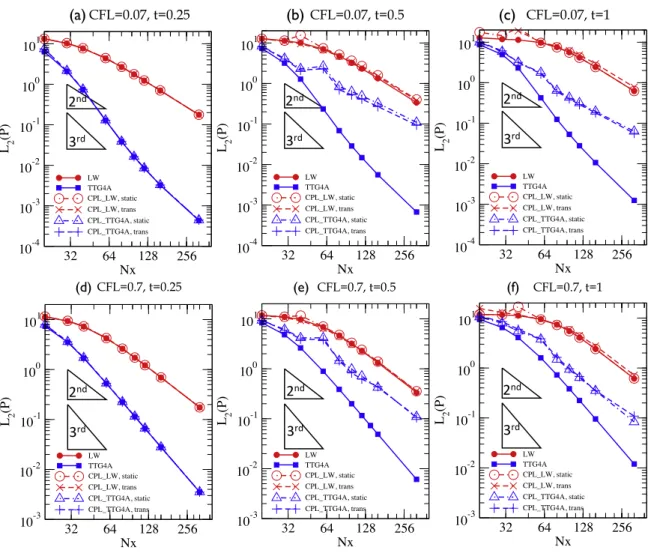
of thecell. Theanalytical fieldsare given byEq. (10)with thevortex center advected tothe anticipatedpositions. Figs. 7 and8show L2(P)and L∞(P)curvesasafunctionofthegridresolutionatthreedimensionlessinstantst=0.25,0.5 and 1,
when the vortex is convected from the initial position x= −10Rc at t=0, to the positions x= −5Rc (upstream of the
interface)att=0.25,x=0 (crossingtheinterface)att=0.5,andx=10Rc (downstreamoftheinterface)att=1.
InFig. 7(a), convergenceatt=0.25 isfirstcheckedforthesmallCFLnumberof0.07.Therearetwosets ofconvergence
G. Wang et al. / Journal of Computational Physics 274 (2014) 333–355 341
Fig. 7. ThequadraticmeanerrorsofinstantaneouspressurefieldsL2(P)versusmeshresolutionNx fordifferentcasesusingtheLWorTTG4Aschemes. Thepressureprofilesarecomparedwiththeanalyticprofileswhenthevortexreaches upstreamof theinterface (t=0.25),theinterface(t=0.5)and thedownstreamoftheinterface(t=1).ThecomputationsareusingtwosetsoftimestepswithCFL=0.07 (top)andCFL=0.7 (bottom).Thetranslation speedsforthetranslatingcoupledcasesisUtrans=200 m/s.
the standard one. As expected, simulations using LW recover the scheme 2nd-order spatial accuracy, while simulations using TTG4A reaches a 3rd-orderaccuracy or slightly above. In Fig. 7(b), convergence results are given at t=0.5. In the
coupled cases, all static and translating (Utrans =200 m/s) have similar error levels and slopes. Since the two domains
are presently coupled by a2nd-order linearinterpolation scheme, only 2nd-order spatialaccuracies are ensured for both LW and TTG4Asimulations. Higher-order interpolationwould be required to achieve higher spatial accuracy.Yet, coupled simulations withTTG4Acontain almostadecade less errorsthan thecoupledLW for any givengrid resolution, asalready evidencedintheabove 1D testcase.InFig. 7(c),att=1,allthecoupledsimulationskeeptheir2nd-orderspatialaccuracy, eventhoughthevortexhastraveled10Rc downstreamtheinterface.Again,themesh-translatingcoupledcaseshavesimilar
errorlevels asthestatic ones.Figs. 7(d)–(f)show thesameconvergedresults forCFL=0.7.All coupledcasesagainexhibit
2nd-orderaccuracybecauseofthe2nd-orderinterpolation(Figs. 7(e)and(f)).Thetranslatingcoupledcasesalsohavesimilar convergencerates asthestaticones.
Temporal evolution ofthe above simulations isnow considered to assessthe spuriouserrors introduced atevery time step bythe moving coupled domains. The following mesh resolution is chosen: Nx=80 ($x=Rc/4=3.89 mm). Fig. 9
shows the time traces of the pressure signals monitored at the middle point of the overall computational domain for different vortex strengths. Fig. 9(a) stresses that alltemporal signals agreewell withthe standardsimulationfor aCFL of 0.07.Onlyhigh-frequencypressurefluctuationsareintroduced bythetranslatinginterfaceasevidencedinthezoom ofthe plot. When a standard FFTof the signal is performed in Figs. 9(b) and (c), these spurious oscillations are identified by a tonearound51.9 kHz independentofthevortex strengthsand thecoupling onlyintroducesthisadditionalhigh-frequency
noise.WhentheCFLisincreasedto0.7inFig. 9(d),thesameconclusionscanbedrawnforallvortexstrengths, exceptthat additionalhumpsappear aroundthetone.
The vortex strength is then set to Γ =0.5 m2/s. The pressure spectra are presented for different translating speeds
Utrans=100,200 and 300 m/s in Fig. 10(a) and for different mesh sizes $x in Fig. 10(b), allcases being summarized in
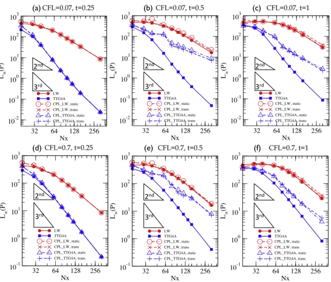
propor-342 G. Wang et al. / Journal of Computational Physics 274 (2014) 333–355
Fig. 8. Themaximumerrorsof instantaneouspressurefields L∞(P)versusmeshresolutionNxfordifferentcasesusingtheLWorTTG4Aschemes.The pressureprofilesarecomparedwith theanalyticprofileswhen thevortexreachesupstreamoftheinterface (t=0.25),theinterface(t=0.5)andthe downstreamof theinterface (t=1).Thecomputationsareusingtwosetsoftime stepswith CFL=0.07 (top)andCFL=0.7 (bottom). Thetranslation speedsforthetranslatingcoupledcasesisUtrans=200 m/s.
Fig. 9. Temporalevolutionsofpressuresignalsatthecentralposition (0, 0)ofinterfacefordifferentvortexintensities(top: Γ=0.5 m2/s;bottom: Γ= 0.036 m2/s)instandard,staticcoupledandtranslating(Utrans=200 m/s)coupledcases.Timetraces(a)andspectra(b)–(c)forCFL=0.07.(d)Spectrafor
G. Wang et al. / Journal of Computational Physics 274 (2014) 333–355 343
Fig. 10. Spectraofpressuresignalsatthecentralposition(0,0)ofinterfaceintranslatingcoupledcases(CFL=0.07;vortexintensityΓ=0.5):(a)with differenttranslatingspeeds,Utrans=100, 200 and 300 m/s andmeshsize $x=Rc/4;(b)withdifferentmeshsizes,$x=Rc/4,Rc/6 and Rc/8 fora translatingspeedUtrans=200 m/s;(c)atdifferentmonitoringpositionsforatranslatingspeedUtrans=200 m/s;(d)usingdifferenttimeratiosαt=38.9, 19.45, 7.78and 3.89.
Table 1
Frequency ftransofpressuresignalspectraintranslatingcoupledcaseswithdifferentmeshsizes $xandtranslatingspeedsUtrans.
$x[mm] Utrans[m/s] ftrans[kHz] Strans= ftransUtrans$x
3.8900 100 25.9 1.0075
3.8900 200 51.9 1.0095
3.8900 300 77.8 1.0088
2.5933 200 77.8 1.0088
1.9450 200 103.8 1.0094
tional to the mesh size, asconfirmed bythe non-dimensional ratio or equivalent Strouhal number obtained as the ratio betweenthesethreeparameters
Strans= ftransUtrans
$x =1.0. (13)
Interpolationerrorisindeedfluctuatingintimeasthepositionofdonorcellsevolveswithtime.Thelevelofthisnumerical noise is however two orders ofmagnitude smallerthan themain vortex signal and can be considered negligible as long asitdoes notinterfere with LESresolvedlarge-scalemotions. Moreover, thishigh frequencynoise decreasesrapidly away fromthemiddlepointasshowninFig. 10(c)and ishigherthan thetypicalfrequenciesofcombustionand turbomachinery noiseofinterest.Finally, Fig. 10(d)clearlyshowsthat theadditional humpsobservedinFig. 9(d) arerelatedto theratio of thetranslationperiod Ttrans tothetimestep$t
αt= Ttrans
$t =
$x/Utrans
CFL· $x/(U0+c0). (14)
On theone hand,biggerαt leadtoless spuriousfrequencybandsinthepressurespectra,andwhen Ttrans iswellresolved
bythetimestep, only thepeaktranslating frequencyat51.9 kHzcanbe seen.Ontheother hand, poorsampling of Ttrans
leadstoaliasingfrequencies [79,83].
3.3. Viscousvortextravelinginastaticandmovingcoupledsimulation
Theviscous vortex[84]validation caseischosen toqualify themomentum diffusionusingfull 2DNavier–Stokes equa-tions. The samesetups as in the previous inviscid vortex problem is used here: thestatic test cases shown in Figs. 6(a) and (b), and themoving coupled caseconsisting of two computationaldomains coupled with MISCOG as inFig. 6(c). An initialvortexwithacoreradius Rc=0.01556 m isimposedusingEq.(10)onaviscousflowwithuniformmeanconvecting
velocity U0=100 m/s.TwoReynoldsnumbers(Re=U0Rc/ν)are chosenRe=102 and Re=1020. The CFLnumber isset to 0.7 andthe two numericalschemes LW and TTG4A aretested for different meshresolutions. The diffusion operatoris
344 G. Wang et al. / Journal of Computational Physics 274 (2014) 333–355
Fig. 11. Viscousvortextraveling case:thetransversevelocityv convectedanddiffusedwithtimetinsimulationsusingLW(a)andTTG4A(b)schemes. Timetisnormalizedby20Rc/U0.Meshsize$x=Rc/4 andRe=102.
Theanalyticalsolutionforthistemporallyevolvingvelocityfieldcanbeobtainedthroughaperturbationanalysisofthe governingequationsdetailedin[85],andreads:
u(x,y,t)=U0− Γ R2c (y−yc) α2 e −r2/2αR2c (15) v(x,y,t)= Γ R2c (x−xc) α2 e −r2/2αR2 c (16)
wheretheparameterα isdefinedas
α=1+2νt/R2c (17)
wherethevortexstrengthisΓ =0.5 m2/s andthedistancer ismeasuredrelativetothevortexcenter(xc, yc)traveling at
U0.Thekinematicviscosity νequals1.52×10−3 or1.52×10−2 m2/s forthetwoReynolds-numbercasesrespectively.
Fig. 11 shows the temporal evolution of the transverse velocity component v along the x-axis. The vortex is initially locatedat x= −10Rc att=0, travelingfrom leftto rightwiththe meanconvectingflowwhiledecayingdueto diffusion.
Thecoupledsimulationhastwocomputationaldomains(indicatedbytwodifferentsymbols)coupledattheinterfacex=0. The vortex core travels through the interface att=0.5 and reachesx=10Rc att=1. The results predictedby the
cou-pledsimulations fitvery wellwith thoseofthestandard referencesimulations. The TTG4Aschemeagreesbetter withthe analyticalsolutionthan theLWscheme,asithaslessnumericaldiffusionand dispersion.
ThevelocityanditsgradientprofilesacrossoralongtheinterfacearefurthercheckedinFig. 12forthetwoschemes.The transverse velocity v iscontinuousacrosstheinterfaceinFigs. 12(a)and (b).All simulationsinalldomainsyieldthesame results. Thesameconclusioncanbedrawn forthelongitudinal velocityu alongtheinterface(x=0)inFigs. 12(c)and (d). Figs. 12(e) to(h) show themagnitudes ofthe gradientsof thetransverse velocity v. Very similar results areobtained for boththecoupledand standardcases.However,thecouplinginterfaceseemstocause aslightdampingofthemagnitudeof thegradients,andthecontinuityofthederivativesisnolonger fulfilledbecauseofthelinearinterpolation.
In Fig. 13 the numerical convergence is again checked by the L2-error and L∞-error on the transverse velocity
field versus mesh resolution Nx by comparing with the exact analytical solution (Eq. (16)). For both Reynolds numbers
Re=1020 and 102 (Figs. 13(b) and (c) respectively), the TTG4A scheme exhibits 3rd-order spatial accuracy and the LW scheme 2nd-order accuracy in avery similar manner asthe inviscid case(Fig. 13(a)). Similarly, the order of thecoupled TTG4Aschemeisreducedto2nd-orderbecauseofthe2nd-order interpolation.
3.4. Flowpastarotatingcylinder
AcompressibleLESofa rotor/statorconfigurationinvolves wakescrossing rotatingboundaries. Thefinalvalidationcase thereforeinvolvesanoverlapping rotatinginterface,andtheflowpastarotatingcylinder. Itisawell-investigated test-case targeting wake dynamics and flow control [86]. Two critical parameters are relevant to this problem: (1) the Reynolds
G. Wang et al. / Journal of Computational Physics 274 (2014) 333–355 345
Fig. 12. Thevelocityanditsgradientprofileswhentheviscousvortextravelsthroughtheinterface att=0.5;analyticalsolution(hardlines),standard referencesimulation(dashedlines)andcoupledsimulation(lineswithsymbols).ThesimulationsareusingtheLW(left)orTTG4A(right)schemes.Mesh size$x=Rc/4 andRe=102.
peripheral velocityratioα=0.5Dω/U0, definedastheratio ofthevelocitymagnitude atthesurfaceofthecylinderωD/2
to the free-stream velocity. The case retained in the following simulation uses Re=200 and α=3.5. For thisoperating
condition,astationarysolutionisexpectedwithtransienteffectsinducedbytheinitialmotionofthecylinder [86]. As shown in Fig. 14, two numerical configurations are again used for the simulation. In Fig. 14(a), a standard stan-dalonesimulationusesasinglerectangulardomainofdimensions[−50D,50D]× [50D,200D]with acylindercenteredat (0,0).Thecylinderboundarycondition isarotatingisothermalwall withaprescribedrotatingwall velocityinthecounter
clockwisedirection ata speedof ω=2αU0/D. Themain flowvalue, U0, isassigned attheupstream boundarywhile the
downstreamoutletusesareferencestaticpressure.InletandoutletboundariesalsouseNSCBC.Thetopandbottom bound-aries are set to beadiabatic slip wall conditions. A close-up view of the unstructured mesh(made of triangular cells)is given inFig. 14(a), with thesmallestcell sizeequalto D/400 located onthe cylindersurface. Thecoupled simulationhas
thesamemeshtopology, but consistsoftwo meshes:one rotatingmesharoundthe cylinderand extendingradially upto
r≤2.25D. Itsrotation speedis fixedatω=2αU0/D and thecylinder wall condition isinthiscasean isothermalno-slip
condition. A static mesh represents the outer domain for r≥1.75D. The two meshes overlap on an annulus located at
r=2D with an overlapping thicknessof 0.5D. The characteristic mesh size is 0.05D inthis region in bothmeshes. The
numericalschemeofbothsimulationsisTTG4A.As mentionedabove, thetwo computationsareimpulsivelystartedfroma uniformfreestreamfieldcoveringthewholedomain.Thetransientiscomputedforatotaldimensionlesstimeof200 (time normalizedbytheconvectivetimeD/U0),untiltheflowhasreachedasteadystate.Theresultsofthecoupledconfiguration
are in excellent agreementwith the standardmethod asevidenced bythe instantaneousvorticity fieldsin Fig. 14 or the axialvelocity U profilesnear the coupledregion and atdifferent instantsin Fig. 15. Transient inducedeffects are further
346 G. Wang et al. / Journal of Computational Physics 274 (2014) 333–355
Fig. 13. QuadraticmeanandmaximumerrorsofinstantaneousfieldsoftransversevelocityL2(v)(a)–(c)andL∞(v)(d)–(f)versusmeshresolutionNxfor differentcasesusingtheLWorTTG4Aschemes.Thetransverseprofilesarecomparedwiththeanalyticprofileswhenthevortexreachestheinterface (t=0.5)forthreedifferentReynoldsnumbers:(a),(d)inviscidvortex;(b),(e)Re=1020;(c),(f)Re=102.
illustrated inFig. 16 where therecordedlift and dragcoefficients temporalevolutions are shownto fully agree whatever the CFDapproach retained. At convergence, thelift and dragcoefficients are CL= −13.41 and CD= −0.03 which isvery
closedtoresultsobtained byMittaland Kumar[86]forthesameconditions,CL= −13.54 andCD= −0.02.
4. LESapplications
As discussedinthe introduction,the motivationforaccurateand efficient couplingstrategiesis toprovide acontrolled numerical formalismallowingfullLESin rotatingmachines.Thelattershouldbeable toaccount forallwave mechanisms in stagesincludingwave generationand propagation. As evidenced inthe previoussections, MISCOG implementedwithin OpenPalm provides an easy to implement extension for existing LES massively parallel solvers as the one developed at CERFACS for bothtranslating and rotatinginterfaces. Toillustratethe feasibilityof LESin suchacontext, two applications are considered,one dealing with wave propagationin alinear cascade(translatinginterface), theother coping with wave interactionandgenerationinarealistic turbinestage(rotatinginterface).
4.1. LESofarotorlinearcascadeforindirectnoisepredictions
Thefirstapplication isthesimulationofthepropagationofacousticand entropywavesinalinearrotorcascadeshown in Fig. 17. This simpler set-up is preferred here as very long simulation times are required to statistically converge the reflectedandtransmittedwavesatlowfrequencies ofinterestincombustionnoise.Thecascadegeometryistakenfromthe mid-spanprofile of theMT1rotor bladedescribed inthenextsection [67,87]. Theselected inlet and outlet relativeMach numbers are0.653 and 0.366 respectively.The inlet and outlet flowangles are −75.76◦ and −60◦ respectively.The inlet
and outlettotal pressures are18.464 and 14.239 barsrespectively.Atranslating speed of500 m/sisimposed tothe rotor blade. The meanflow issubject to a modulated inflow or outflow condition with eitheracoustic or entropy plane waves in thestationary frameas detailedbyDuran and Moreau [88]. As before, these pulsatedwaves areimposed usingNSCBC boundaryconditions.Periodicboundaryconditionsareusedonthesideedges ofthecomputationaldomain.
G. Wang et al. / Journal of Computational Physics 274 (2014) 333–355 347
Fig. 14. Simulationsof aRe=200 flowpastarotatingcylinder:iso-contoursofvorticityarepredictedby(a)singledomainsimulation(b)twodomain coupledsimulationand(c)MittalandKumar[86]simulation.Theratiooftherotatingsurfacespeedandfreestreamspeedαis3.5.Thepresentedzoom nearthecylinder [−3.5D,3.5D] × [−5D,9D]isextractedfromtheentirecomputationaldomain [−50D,50D] × [50D,200D].
Fig. 15. Velocityprofilesalongaverticallinepositionedatx=2D (showninFig. 14)atdifferentinstantst=10,20 and200 ofthesimulations.Continuous linesdenotethestandardstand-alonesimulationapproach.Symbolsrefertothecoupledsimulationresults:staticpart(!)androtatingpart(1).
Threedifferent simulationsare performedwithAVBPusingtheTTG4Ascheme.First afixedmesh servesasa reference calculation asin the above test cases. A second methodinvolves continuously deforming themesh in themoving region around the blade. More details on the application of this Arbitrary Lagrangian–Eulerian (ALE) method can be found in Duran andMoreau [88].FinallytheMISCOG methodis appliedwithtranslating interfaces.As showninFig. 17anentropy wave or equivalently the temperature fluctuation is applied at the fixed inlet location. These waves are then traveling from left to right because of the mean inflow velocity field and create two acoustic waves (one reflected and the other transmitted)whengoing throughtherotorbladepassage.This isthesourceofindirectcombustion noiseinthefirststage of an actual turbine [89,90]. Similar results have been obtained with acoustic waves imposed either at the inlet or the