HAL Id: hal-01373867
https://hal.archives-ouvertes.fr/hal-01373867
Submitted on 29 Sep 2016HAL is a multi-disciplinary open access archive for the deposit and dissemination of sci-entific research documents, whether they are pub-lished or not. The documents may come from teaching and research institutions in France or abroad, or from public or private research centers.
L’archive ouverte pluridisciplinaire HAL, est destinée au dépôt et à la diffusion de documents scientifiques de niveau recherche, publiés ou non, émanant des établissements d’enseignement et de recherche français ou étrangers, des laboratoires publics ou privés.
Parametric shape modeler for hulls and appendages
Elisa Berrini, Bernard Mourrain, Yann Roux, Guillaume Fontaine, Eric Jean
To cite this version:
Elisa Berrini, Bernard Mourrain, Yann Roux, Guillaume Fontaine, Eric Jean. Parametric shape modeler for hulls and appendages. COMPIT’16, May 2016, Lecce, Italy. pp.255-263. �hal-01373867�
1
Parametric shape modeler for hulls and appendages
Elisa Berrini, Inria / MyCFD, Sophia-Antipolis/France, [email protected] Bernard Mourrain, Inria, Sophia-Antipolis/France, [email protected]
Yann Roux, MyCFD, Sophia-Antipolis/France, [email protected]
Guillaume Fontaine, K-Epsilon, Sophia-Antipolis/France, [email protected] Eric Jean, Profils, Marseille/France, [email protected]
Abstract
This paper describes a parametric shape modeler tool for deforming hulls and appendages, with the purpose of being integrated into an automatic shape optimization loop with a CFD solver. The modeler allows generating shapes by controlling the parameters of a twofold parameterization: geometrical – based on a skeleton approach – and architectural – based on the design practice and effects on the object’s performance. The resulting forms are relevant and valid thanks to a smoothing term to ensure shape consistency control. Thanks to this approach, architects can directly use a NURBS CAD model in the modeler tool and will obtain variations of the initial design to improve performance without additional work. The methodology developed can be applied to any shape that can be described by a skeleton, e.g. hulls, foils, bulbous bows, but also wind turbines, airships, etc. The skeleton consists of a set of B-Spline curves composed of a generating curve and section curves. The deformation of the shape is performed by changing explicit parameters of the representation or implicit parameters such as architectural parameters. The new shape is obtained by minimizing a distance function between the current parameters and the target’s in combination with a smoothing term to assure shape consistency control. Finally, the 3D surface wrapping the skeleton is rebuilt using surface network technics. This paper presents the general methodology and an example of application to a bulbous bow on a fishing trawler, with RANSE CFD computations to determine the best design.
1. Introduction
Automatic shape optimization is a growing field of study, with applications in various industrial sectors. As the performances of a flow-exposed object can be obtained accurately with CFD (Computational Fluid Dynamics), small changes in design can be captured and analysed. To exploit these performance analysis capabilities, it is important to have a precise and efficient control of the geometry of the objects. The results of the modelling/analysis process rely on two main ingredients. To evaluate with accuracy the hydrodynamic properties of a hull, accurate flow solvers are required. Free surface needs to be captured precisely, as well as turbulent flow phenomena. Reynolds-averaged Navier-Stokes (RANS) solvers, completed with a powerful grid generator, are well adapted to capture accurately the flow around complex objects.
To improve the form of a hull in order to increase its performances, a precise shape consistency control is essential when performing deformations. Naval architects need to use shape quality preserving tools to modify hulls avoiding non-realistic forms.
The coupling of an accurate flow solver and a quality preserving shape modeler is the basis for an efficient automatic shape optimization loop. An optimisation algorithm can optionally complete the loop to determine automatically new shape parameter values according to the CFD results.
We propose a parametric shape modeler tool for deforming objects, with the purpose of being integrated into an automatic shape optimization loop with a CFD solver. Our tool has the ability to generate valid forms from an architectural point of view thanks to an innovative shape consistency control based on architectural parameters. A skeleton composed of a generating curve and a family of section curves represents the object. The generalizable concept of skeleton-based approach allows us
2 to apply our tool to a large selection of shapes e.g. hulls, foils, bulbous bows, propellers, wind turbines, airships, etc.
In this paper we present an application to the bulbous bow of a fishing trawler ship. The aim is to reduce the total drag of the hull thanks to bulb form variations. With the parametric modeler, we create a set of shapes exploring the parameters domain and use RANSE CFD computations to determine the best design.
2. Related work
Optimising the shape of the bulbous bow has been seen as an efficient way to reduce the drag of a hull, and thus the costs of exploitation of the ship, since several years. The coupling of a flow solver to a modeler and an optimisation algorithm is a widely used methodology. Some of the previous work can be seen in Valdenazzi (2003), Hochkirch (2009), Blanchard (2013).
Shape deformation for ships is a relatively recent approach. However, deformation techniques have been wildly developed in other application fields, such as 3D animations or movies.
Free Form Deformation – FFD – and morphing are classical methods created for 3D animations purposes, and they have been applied to shape optimization for ships. Morphing generates shapes interpolated from two extremal ones. Such a methodology allows to explore a precise panel of shapes if the architect has a clear idea of the extremal values. FFD consist in enclosing the object within a simpler hull, usually a cube as described by Sederberg (1986), then the object is transformed when the hull is modified. FFD is applied to ship hulls by Kang (2012), Peri (2013). FFD and morphing are usually applied to meshes and not a continuous geometry in a naval context, thus limiting deformation because the meshes can be subject to degeneration. FFD method can be very efficient with a small number of degrees of freedom to control the whole shape of the object. However, in order to perform local deformations, the only way is to increase the number of control points by refining the areas of interest. Moreover, FFD does not take into account any architectural parameters when deforming an object, leading possibly to non-realistic results.
Engineering dedicated CAD software recently provides parametric design features, allowing the user to build parametrized models such as CatiaTM or GrasshopperTM for Rhinoceros 3DTM. When these
parameters are modified, the corresponding elements of the object are modified. Thanks to the relationship between elements, the deformation propagates throughout the whole model.
Specific software have been developed during the last decades for ship applications. One of the most widespread is CAESESTM form Friendship Systems, allowing the user to create geometries using
advanced parameters that can be modified easily by hand or automatically with a CFD optimization loop as described by Papanikolaou (2011). Similarly, a ship dedicated tool Bataos, used by Jacquin
(2003) allows to modify the shape of sections of the hull by multiplying or adding predefined
functions to the control points the B-Spline curve describing the section.
The aim of our tool is to be used without any human interaction once an original geometric model is available, independently of the way it is built and of its quality.
3. Parametric modeler
To obtain smoothly deformed shapes, we propose a new modeler tool based on a generic methodology, allowing us to describe a large panel of objects in the same way. We parameterize shape with a generic skeleton concept, completed by specific architectural parameters according to the studied shape.
3 3.1. Shape parameterization
3.1.1. Geometrical parametrisation
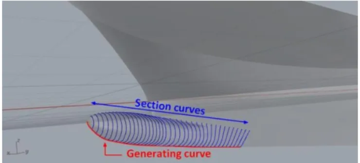
The skeleton consist of a set of B-Spline curves composed of generating curve and section curves. The purpose of the generating curve is to describe the general shape of the object. The sections are similar to the classic architect’s line plan, describing more precisely the outlines of the object around the generating curve. Once the generating curve is identified on the CAD model, sections are computed as intersections between the studied object and a family of planes along the generating curve. A fitting process is used, inspired by Wang (2000), to create the B-Spline curves that approximate the intersection curves.
Figure 1 – Skeleton of a bulbous bow
3.1.2. Architectural parameters
We define a set of architectural parameters on the studied object according to the design practice and effects on the object performance. The strategy of our modeler is to control the whole shape through these parameters. Both generating curve and section curves have an independent set of parameters, as illustrated in Figure 2 and Figure 3. In this example the length, the angle, the height and width are relevant parameters to control the shape of a bulbous bow. Our model allows to enrich the parameter set with new kinds of parameters, such as the value of sectional areas included for each section.
Figure 2 – Generating curve parameters Figure 3 – Section parameters We introduce an observer function 𝜙 that computes the set of parameters 𝑃 on a given geometry 𝐺: 𝜙: 𝐺 ⟶ 𝑃. For the generating curve the parameters are real and finite values whereas sections describe parameters as a function along the generating curve, thus defining 𝜙 in an infinite dimensional space. In order to reduce the dimension of 𝜙 we represent the functions of parameters with B-Spline curves with a small number of control points.
3.2. Shape deformation
In our methodology, deforming an object corresponds to finding a new geometry 𝐺 that matches a given set of architectural parameters 𝑃. Referring to the definition of the observer function 𝜙, to deform a shape we need to compute 𝜙−1: 𝑃 ⟶ 𝐺. Starting from the B-Spline description of the
4 until the current parameters matches the target one, for the generating curve and the section curves independently. This problem can be defined as a non-linear constrained optimization problem, the control point coordinates being the solution of a specific minimization system.
The minimisation system is built with four terms:
1. The first term 𝐸𝑝𝑎𝑟𝑎𝑚 measures the distance of the current parameters values to the target ones.
2. The second term 𝐸𝑠ℎ𝑎𝑝𝑒 is introduced to ensure consistency control by measuring the distance of
the current generating or section curve to the original one.
3. The third term allows taking into account specific constraints 𝐹 for the studied object, usually position or tangency constrains. These constraints are defined for each section and are not necessarily the same for all sections. For a bulbous bow, as we use a half hull, we have to ensure that the section curves end in a plane (here 𝑌 = 0) and that the tangent at the extremity along the vessel centerline are preserved.
4. The last term controls the overall smoothness of the shape by introducing stiffness between successive control points. It consist in correction terms 𝑀𝑙 to control respectively 𝒞1 and 𝒞2
properties of control points.
The definition of the problem is well adapted to Sequential Quadratic Programming (SQP). SQP algorithm uses Newton’s method to find roots of the gradient. We start with the original curve as the starting point of the algorithm, then we decrease the shape consistency term and the smoothing control term at each iteration and start the SQP again with the last computed curve. The algorithm stops when the value of the objective function reaches a fixed threshold.
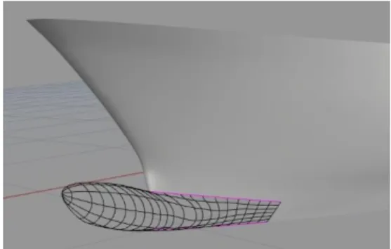
3.3. Surface reconstruction
The optimization method outputs deformed sections and generating curves, corresponding to the skeleton of a new shape. To evaluate the shape performances with a CFD solver, we first need to reconstruct the 3D surface wrapping the deformed skeleton. Moreover, building a new surface allows to obtain a cleaned-up model for the meshing tool.
For complex objects, multi-patch surfaces are required. In such cases, a particular attention has to be given to the continuity between them: for our application, patches have to be at least 𝒞1. We chose to
focus on Surface Network technique, described by Piegl (1997), which ensures the continuity between adjacent surfaces by building the curve grids with specific tangency constraints on the boundary. The computed grid is illustrated in Figure 4.
5 4. Numerical methods
4.1. Mesh generation
To generate non-conformal full hexahedral unstructured meshes on complex arbitrary geometries, we use HEXPRESSTM from Numeca International. In addition, the advanced smoothing capability
provides high-quality boundary layers insertion, Wackers (2012). The software HEXPRESSTM creates
a closed water-tight triangularized volume, embedding the ship hull, then a body-fitted computational grid is build.
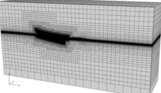
One of the meshes used in our simulations is shown in Figure 5 and Figure 6. The grid generation process requires clean and closed geometries to provide robust meshes. Thanks to the shape consistency control and the smooth reconstruction of surfaces, the modeler generates shapes which are well-adapted to these requirements and which allows to produce high-quality meshes for computations.
During the computation, the automatic mesh refinement has been used. Automatic, adaptive mesh refinement is a technique for optimising the grid in the simulation, by adapting the grid to the flow as it develops during the simulation to increase the precision locally. This is done by locally dividing cells into smaller cells, or if necessary, by merging small cells back into larger cells in order to undo earlier refinement. During the computation, the number of cells increases from 1.9 to approximatively 2.2 million cells, for a half hull mesh. Figure 5 shows a view of the whole grid and Figure 6 shows the mesh refinement around the hull and the free surface at the end of the computation.
Figure 5 – General view of the mesh and the
computational domain Figure 6 – Mesh around the hull
4.2. Flow solver
ISIS-CFD, available as a part of the FINETM/Marine computing suite, is an incompressible, unsteady
Reynolds-averaged Navier-Stokes (RANS) solver. For the turbulent flow, additional transport equations for the modeled variables are discretized and solved. The two-equation k-ω SST linear eddy-viscosity model of Menter is used for turbulence modeling. The solver is based on the finite volume method to build the spatial discretisation of the transport equations. The unstructured discretisation is face-based, which means that cells with an arbitrary number of arbitrarily shaped faces are accepted. This makes the solver ideal for adaptive grid refinement, as it can perform computations on locally refined grids without any modification.
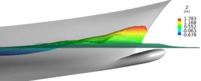
Free-surface flow is simulated with a multi-phase flow approach: the water surface is captured with a conservation equation for the volume fraction of water, discretised with specific compressive discretisation schemes, Queutey (2007). The vessels dynamic trim and sinkage are resolved during the simulation.
6 Figure 7 – Free surface elevation
5. Application on bulbous bow deformation
We aim to reduce the total drag of a fishing trawler ship thanks to variations of its bulbous bow shape. Starting from a first geometry of the hull with a bulbous bow, see Figure 8, we generate a set of shape variations with the parametric modeler. Then the total drag of each shape is computed with ISIS-CFD. We use this initial set of data to build a Design of Experiments (DOE) on which we will apply a response surface methodology, as explained by Jones (2011), to explore new design possibilities. The DOE can be seen as a database of objective function values, here the total drag of the hull, associated to design parameter values, which are the architectural parameters used in the modeler. The response surface methodology then allows us to compute an estimate value of the objective function for any parameters included in the database bounds. To sample the design parameter values of the database, we use a Latin Hypercube distribution Iman (1981).
We describe the construction of the Latin Hypercube in the following section, then we present the corresponding results computed with ISIS-CFD.
5.1. Deformations of the bulbous bow
We chose three parameters to control the bulb shape: the length and angle of the generating curve (see Figure 2) and the width of the sections (see Figure 3). Deformations are parameterized as percentages of the initial parameters values. We describe the limits of the exploration domain in Table I:
Table I – Limits of parameters domain
Length Angle Width
Initial value 1.61 m 31.52° 0.83 m (value at mid-bow) Min variation 15% (=1.86m) -25% (=23.64°) -20% (=0.66 m)
Max variation 90% (=3.07m) 0% (=31.52°) 20% (=0.99 m)
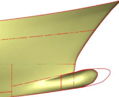
The initial bulb being quite short, we assumed that shapes with a lower length than 1.86m will not positively influence the drag, likewise we restricted the bulb to not be longer than the extremity of the upper bow. For the angle, we noticed that when the length of the bow is increased, keeping the original value will cause the bulb to pierce the free surface, again this configuration is unwanted. From the bounds described in Table I, intermediary values are computed with a Latin Hypercube method. We illustrate in Figure 8 the initial hull (yellow) with a one of the variation (red) included in the Latin Hypercube (Length: +42.86% ; Angle: -23.08% ; Width: +0.0%).
7 Figure 8 – Initial hull (yellow) vs. a bulbous bow shape variation (red)
5.2. RANS CFD results
The studied trawler ship has a length at waterline of 22.35 metres and a displacement of 150 metric tons. Simulations are done at a speed of 13 knots (6.688m/s). Trim and sinkage are solved, while the hull speed is imposed according to a ¼ sinusoidal ramp law. Fluid characteristics are the following:
𝜌 (kg/m3) 𝜇 (Pa.s)
Water 1026.02 0.00122 Air 1.2 1.819 * 10-5
We present in Table II the results obtained from the Latin Hypercube distribution. Table II represents the Design of Experiments used for the response surface methodology.
Table II – Drag results for the different bulbous bow shapes # Length variation (%) Angle variation (%) Width variation (%) Total Drag (N) Pressure drag (N) Viscous drag (N) % reduction in total drag from original hull 0 0.0000 0.0000 0.0000 73740 63853 9887 0% 1 0.4286 -0.2308 0.0000 71760 61848 9912 2.69% 2 0.8571 0.0000 0.0000 72120 62196 9924 2.20% 3 0.4670 -0.2180 0.084 71428 61451 9977 3.13% 4 0.5069 -0.1821 -0.1786 72441 62508 9933 1.76% 5 0.1944 -0.1026 -0.0467 73015 63186 9829 0.98% 6 0.5349 -0.1252 -0.1364 72479 62490 9989 1.71% 7 0.3807 -0.0861 -0.106 71440 61453 9987 3.12% 8 0.1704 -0.1688 0.164 72603 62701 9902 1.54% 9 0.2693 -0.2262 0.0445 72027 62142 9885 2.32% 10 0.3464 -0.1091 -0.0289 72266 62414 9853 2.00% 11 0.6319 -0.0887 0.1853 71676 61513 10163 2.80% 12 0.6717 -0.1514 -0.1711 72312 62261 10051 1.94% 13 0.2381 -0.1368 0.0324 72037 62200 9837 2.31% 14 0.6777 -0.1411 -0.0069 71634 61588 10046 2.86% 15 0.5870 -0.1981 0.0999 71054 60971 10083 3.64% 16 0.3110 -0.1717 0.1365 71660 61714 9946 2.82% 17 0.4391 -0.2095 -0.0818 72380 62484 9896 1.84%
8 We illustrate the surface elevation of the best results (#3, #7 and #15) in Figure 9, Figure 10 and Figure 11.
Figure 9 – Free surface elevation for case #3
Figure 10 – Free surface elevation for case #7
Figure 11- Free surface elevation for case #15 The response surface can be used as a surrogate model on which we can solve an optimization problem: we can find its minima using a genetic algorithm. Those minima give the parameter values that potentially improve the objective function values, here the total drag of the hull.
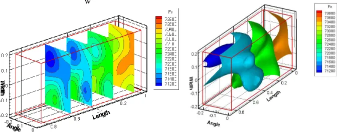
Figure 12 and Figure 13 show a graphical representation of the response surface. Figure 12 represents cutting planes of the design space, showing two main local minima. In Figure 13, we show iso-values of the total drag Fx. We can identify a region where the objective function is predicted to be smaller than in the other part of parameter domain.
w
Figure 12 – Cut planes of the response surface Figure 13 – Iso values of the total drag Fx in the response surface
We identify one of the minimum though a genetic algorithm corresponding to the following parameters values: Length: +60.3% ; Angle: +0% ; Width: +9.36%. The response surface predicted a drag of 71019.58 N. We performed a new ISIS-CFD computation with a geometry corresponding to the new parameters values and we obtained a real total drag value of 71553.21 N, representing 2.97 % of drag reduction from the original bulbous bow. To obtain better results, two strategies have to be developed: first the response surface has to be enriched by new values in order to represent more accurately the real distribution of drag according to the parameters. Then more advanced methods to find the point of maximum interest in the response surface can be used. For example, algorithms based on Kriging such as Efficient Global Optimization find minima on a surrogate models by maximizing the probability of improvement of the objective function as shown in Jones (1998) and Duvigneau
9 6. Conclusion and future work
This paper presents a method for smooth shape deformation. The twofold parametrization, geometrical and architectural, demonstrates its capability to generate simulation-suited models with large possible shape domain. The skeleton based approach allows us to use the developed methodology to different kind of objects, e.g. hulls, foils, bulbous bows, propellers, wind turbines, airships, etc.
Further work will focus on the link with CFD solvers. A fully automated optimization loop will be developed. With the integration of an optimization algorithm as Efficient Global Optimization, the process of finding minima on the surrogate model would be significantly improved.
7. Acknowledgements
The project was achieved with the financial support of ANRT (Association Nationale de la Recherche et de la Technologie).
8. References
BLANCHARD, L. ; BERRINI, E. ; DUVIGNEAU, R. ; ROUX, Y. ; MOURRAIN, B. ; JEAN, E. (2013) Bulbous bow shape optimization. 5th International Conference on Computation Mehtods in Marine Engineering (Marine 2013), pp. 412–423.
DUVIGNEAU, R.; CHANDRASHEKAR, P. (2012) Kriging-based optimization applied to flow
control. International Journal for Numerical Methods in Fluids 69/11, pp. 1701–1714.
HOCHKIRCH, K; BERTRAM, V. (2009) Slow Steaming Bulbous Bow Optimization for a Large
Containership. COMPIT 2009: Conf. Computer and IT Appl. Maritime Ind, pp. 390–389
IMAN, R.L.; HELTON, J.C.; CAMPBELL, J.E. (1981). An approach to sensitivity analysis of
computer models, Part 1. Introduction, input variable selection and preliminary variable assessment.
Journal of Quality Technology 13/3, pp.174–183.
JACQUIN, E. ; ALESSANDRINI, B. ; BELLEVRE, D. ; CORDIER, S. (2003) Nouvelle méthode de
design des carnes de voiliers de compétition. 9ème Journée de l’hydrodynamique.
JONES, D.R.; SCHONLAU, M.; WELCH, W.J. (1998) Efficient global optimization of expensive
black-box functions. Journal of Global Optimization 13/4, pp. 455–492.
JONES, D. R. (2001) A Taxonomy of Global Optimization Methods Based on Response Surfaces, Journal of Global Optimization, 21/4, pp. 345–383
KANG, J.; LEE, B. (2012), Geometric interpolation and extrapolation for rapid generation of hull
forms. COMPIT 2012: Conf. Computer and IT Appl. Maritime Ind, pp. 202–212.
PAPANIKOLAOU, A.; HARRIES, S.; WILKEN, M.; ZARAPHONITIS, G. (2011) Integrated ship
design and multiobjective optimization approach to ship design. International Conference on
Computer Applications in Shipbuilding
PERI, D.; DIEZ, M. (2013) Robust design optimization of a monohull for wave wash minimization. 5th International Conference on Computation Mehods in Marine Engineering (Marine 2013), p. 89–100. PIEGL, L.; TILLER, W. (1997) The NURBS Book (2Nd Ed.). New York, NY, USA: Springer-Verlag New York, Inc.
10 QUEUTEY, P; VISONNEAU. M. (2007) An interface capturing method for free-surface
hydrodynamic flows. Computers & Fluids, 36/9, pp. 1481–1510.
SEDERBERG, T.W.; PARRY, S.R (1986). Free-form deformation of solid geometric models. SIGGRAPH Comput Graph 20/4, pp. 151–160.
VALDENAZZI, F.; HARRIES, S.; JANSON, C.E.; LEER-ANDERSEN, M.; MAISONNEUVE, J.J.; MARZI, J.; RAVEN, H. (2003) The fantastic RORO: CFD optimization of the forebody and its
experimental verification.NAV2003
WACKERS, J; DENG, G.B.; LEROYER, A.; QUEUTEY, P. ; VISONNEAU, M. (2012) Adaptive
grid refinement algorithm for hydrodynamic flows. Computers & Fluids 55, pp. 85–100.
WANG, W.; POTTMANN, H.; LIU, Y. (2006) Fitting b-spline curves to point clouds by