HAL Id: hal-00748939
https://hal.archives-ouvertes.fr/hal-00748939
Submitted on 6 Nov 2012
HAL is a multi-disciplinary open access
archive for the deposit and dissemination of
sci-entific research documents, whether they are
pub-lished or not. The documents may come from
teaching and research institutions in France or
abroad, or from public or private research centers.
L’archive ouverte pluridisciplinaire HAL, est
destinée au dépôt et à la diffusion de documents
scientifiques de niveau recherche, publiés ou non,
émanant des établissements d’enseignement et de
recherche français ou étrangers, des laboratoires
publics ou privés.
Non-parametric estimation of the coefficients of ergodic
diffusion processes based on high-frequency data
Fabienne Comte, Valentine Genon-Catalot, Yves Rozenholc
To cite this version:
Fabienne Comte, Valentine Genon-Catalot, Yves Rozenholc. Non-parametric estimation of the
co-efficients of ergodic diffusion processes based on high-frequency data. M. Kessler, A. Lindner, M.
Sorensen. Statistical Methods for Stochastic Differential Equations, Chapman & Hall/CRC
Mono-graphs on Statistics & Applied Probability, pp.341-381, 2012, SemStat series. �hal-00748939�
Non-parametric estimation
of the coefficients of
ergodic diffusion processes
based on high-frequency data
Fabienne Comte, Valentine Genon-Catalot and Yves Rozenholc UFR de Math´ematiques et Informatique, Universit´e Paris Descartes – Paris 5
45 rue des Saints-P`eres, 75270 Paris cedex 06, France
5.1 Introduction
The content of this chapter is directly inspired by Comte, Genon-Catalot, and Rozenholc (2006; 2007). We consider non-parametric estimation of the drift and diffusion coefficients of a one-dimensional diffusion process. The main assumption on the diffusion model is that it is ergodic and geometrically β-mixing. The sample path is assumed to be discretely observed with a small regular sampling interval∆. The estimation method that we develop is based on a penalized mean square approach. This point of view is fully investigated for regression models in Comte and Rozenholc (2002, 2004). We adapt it to discretized diffusion models.
5.2 Model and assumptions
Let(Xt)t≥0be a one-dimensional diffusion process with dynamics described
by the stochastic differential equation:
dXt= b(Xt)dt + σ(Xt)dWt, t≥ 0, X0= ⌘, (5.1)
where(Wt) is a standard Brownian motion and ⌘ is a random variable
inde-pendent of(Wt). Consider the following assumptions: 341
[A1]−1 l < r +1, b and σ belong to C1((l, r)), σ(x) > 0 for all x2 (l, r).
[A2] Forx0, x2 (l, r), let s(x) = exp (−2Rxx0b(u)/σ
2(u)du) denote the scale
density andm(x) = 1/[σ2(x)s(x)] the speed density. We assume
Z l s(x)dx = +1 = Z r s(x)dx, Z r l m(x)dx = M <1. [A3] The initial random variable⌘ has distribution
⇡(x)dx = m(x)/M 1(l,r)(x)dx.
Under [A1] – [A2], equation (5.1) admits a unique strong solution with state space the open interval(l, r) of the real line. Moreover, it is positive recur-rent on this interval and admits as unique stationary distribution the normal-ized speed density⇡. With the additional assumption [A3], the process (Xt) is
strictly stationary, with marginal distribution⇡(x)dx, ergodic and β-mixing, i.e.limt!+1βX(t) = 0 where βX(t) denotes the β-mixing coefficient of
(Xt). For stationary Markov processes such as (Xt), the β-mixing coefficient
has the following explicit expression βX(t) =
Z r l
⇡(x)dxkPt(x, dx0)− ⇡(x0)dx0kT V. (5.2)
The normk.kT V is the total variation norm andPtdenotes the transition
prob-ability (see e.g. Genon-Catalot, Jeantheau, and Lar´edo (2000) for a review). The statistical study relies on a stronger mixing condition which is satisfied in most standard models.
[A4] There exist constantsK > 0 and ✓ > 0 such that:
βX(t) Ke−✓t. (5.3)
In some cases, assumption [A4] can be checked directly using formula (5.2) (see Proposition 5.14 below). Otherwise, simple sufficient conditions are avail-able (see e.g. Proposition 1 in Pardoux and Veretennikov (2001)). Lastly, we strengthen assumptions onb and σ to deal altogether with finite or infinite boundaries and keep a general, simple and clear framework. We also need a moment assumption for⇡ and that σ be bounded.
[A5] LetI = [l, r]\ R.
(i) Assume thatb 2 C1(I), b0bounded onI, σ2 2 C2(I), (σ2)00bounded
onI.
(ii) For allx2 I, σ2(x) σ2 1.
[A6] E(⌘8) <1.
Lemma 5.1 Under Assumptions [A1] – [A3] and [A5] – [A6], for allt, s such
that|t − s| 1, for 1 i 4, E((Xt− Xs)2i) c|t − s|i.
Proof. Using the strict stationarity, we only need to study E((Xt− X0)2i) for
t 1. By the Minkowski inequality, (Xt− X0)2i 22i−1[( Z t 0 b(Xs)ds)2i+ ( Z t 0 σ(Xs)dWs)2i].
For the drift term, we use the H¨older inequality, [A5] and the strict stationarity to get: E ( Z t 0 b(Xs)ds)2i $ t2i−1Z t 0 E(b2i(Xs))ds t2iC(1 + E(⌘2i)),
withC a constant. For the diffusion term, we use the Burkholder–Davis–Gundy inequality and obtain:
E ( Z t 0 σ(Xs)dWs)2i $ C E( Z t 0 σ2(Xs)ds)i C tiσ12i
withC a constant. This gives the result.
5.3 Observations and asymptotic framework
We assume that the sample pathXtis observed atn + 1 discrete instants with
sampling interval∆. The asymptotic framework that we consider is the context of high-frequency data: the sampling interval∆ = ∆ntends to0 as n tends
to infinity. Moreover, we assume that the total lengthn∆nof the time interval
where observations are taken tends to infinity. This is a classical framework for ergodic diffusion models: it allows us to estimate simultaneously the drift b and the diffusion coefficient σ and to enlighten us about the different rates of estimation of these two coefficients. For the penalized non-parametric method developed here, the asymptotic framework has to fulfill the following strength-ened condition.
[A7] Asn tends to infinity, ∆ = ∆n! 0 and n∆n/ ln2n! +1.
To simplify notations, we will drop the subscript and simply write∆ for the sampling interval.
5.4 Estimation method
5.4.1 General description
We aim at estimating functionsb and σ2of model (5.1) on a compact subset
assume from now on that
A = [0, 1], and we set
bA= b1A, σA= σ1A. (5.4)
The estimation method is inspired by what is done for regression models (see e.g. Comte and Rozenholc (2002, 2004)). Suppose we have observations (xi, yi), i = 1, . . . , n such that
yi= f (xi) + noise, (5.5)
wheref is unknown. We consider a regression contrast of the form t! γn(t) = 1 n n X i=1 (yi− t(xi))2.
The aim is to build estimators forf by minimizing the least-square criterion γn(t). For that purpose, we consider a collection of finite dimensional linear
subspaces of L2([0, 1]) and compute for each space an associated least-squares estimator. Afterwards, a data-driven procedure chooses from the resulting col-lection of estimators the “best” one, in a sense to be precised, through a pe-nalization device. For adapting the method to discretized diffusion processes, we have to find a regression equation analogous to (5.5), i.e. find forf = b, σ2
the appropriate couple(xi, yi) and the adequate regression equation. Of course,
starting with a diffusion model, we do not find an exact regression equation but only a regression-type equation, one for the drift and another one for the diffu-sion coefficient. Hence, estimators forb and for σ2are built from two distinct
constructions and the method does not require one to estimate the stationary density⇡.
5.4.2 Spaces of approximation
Let us describe now some possible collections of spaces of approximation. We focus on two specific collections, the collection of dyadic regular piecewise polynomial spaces, denoted hereafter by [DP], and the collection of general piecewise polynomials, denoted by [GP], which is more complex. As for nu-merical implementation, algorithms for both collections are available and have been implemented on several examples.
In what follows, several norms for[0, 1]-supported functions are needed and the following notations will be used:
ktk = (R01t2(x)dx)1/2, ktk⇡= (
R1
0 t2(x)⇡(x)dx)1/2,
ktk1= supx2[0,1]|t(x)|.
(5.6) By our assumptions, the stationary density⇡ is bounded from below and above
on every compact subset of(l, r). Hence, let ⇡0, ⇡1 denote two positive real
numbers such that,
8x 2 [0, 1], 0 < ⇡0 ⇡(x) ⇡1. (5.7)
Thus, for[0, 1]-supported functions, the normsk.k and k.k⇡are equivalent.
Dyadic regular piecewise polynomials
Letr≥ 0, p ≥ 0 be integers. On each subinterval Ij = [(j− 1)/2p, j/2p),
j = 1, . . . , 2p, considerr + 1 polynomials of degree `, '
j,`(x), ` = 0, 1, . . . r
and set'j,`(x) = 0 outside Ij. The spaceSm, m = (p, r), is defined as
generated by theDm= 2p(r + 1) functions ('j,`). A function t in Smmay be
written as t(x) = 2p X j=1 r X `=0 tj,`'j,`(x).
The collection of spaces(Sm, m2 Mn) is such that, for rmaxa fixed integer,
Mn={m = (p, r), p 2 N, r 2 {0, 1, . . . , rmax}, 2p(rmax+ 1) Nn}.
(5.8) In other words,Dm NnwithNn n. The maximal dimension Nn will
be subject to additional constraints. The role ofNnis to bound all dimensions
Dm, even whenm is random. In practice, it corresponds to the maximal
num-ber of coefficients to estimate. Thus it must not be too large.
More concretely, consider the orthogonal collection in L2([−1, 1]) of Legen-dre polynomials(Q`, ` ≥ 0), where the degree of Q` is equal to `,
gener-ating L2([−1, 1]) (see Abramowitz and Stegun (1972), p.774). They satisfy |Q`(x)| 1, 8x 2 [−1, 1], Q`(1) = 1 and R−11 Q2`(u)du = 2/(2` + 1).
Then we setP`(x) = (2` + 1)1/2Q`(2x− 1), to get an orthonormal basis of
L2([0, 1]). Finally,
'j,`(x) = 2p/2P`(2px− j + 1)1Ij(x), j = 1, . . . , 2
p, ` = 0, 1, . . . , r.
The spaceSmhas dimensionDm = 2p(r + 1) and its orthonormal basis
de-scribed above satisfies & & & & & & 2p X j=1 r X `=0 '2j,` & & & & & & 1 Dm(r + 1).
Hence, using notations (5.6), for allt2 Sm,ktk1 (r + 1)1/2D1/2m ktk.
with a single spaceSm. In particular, sinceNn n, the following holds: Σ = X m2Mn exp (−Dm) = rXmax r=0 X p:2p(r+1)N n exp (−2p(r + 1)) <1. (5.9)
Finally, let us sum up the two key properties that are fulfilled by this collection. The collection(Sm)m2Mnis composed of finite dimensional linear sub-spaces
of L2([0, 1]), indexed by a setMndepending onn. The space Smhas
dimen-sionDm Nn n, 8m 2 Mn, whereNndesignates a maximal dimension,
andSmis equipped with an orthonormal basis('λ)λ2Λm with|Λm| = Dm.
The following holds:
(H1) Norm connection: There existsΦ0> 0, such that,
8m 2 Mn,8t 2 Sm,ktk1 Φ0D1/2m ktk. (5.10)
(H2) Nesting condition: There exists a space denoted bySn, belonging to the
collection, with8m 2 Mn, Sm⇢ Sn, with dimension denoted byNn.
In Birg´e and Massart (1998, p.337, Lemma 1), it is proved that property (5.10) is equivalent to:
There existsΦ0> 0,k
X
λ2Λm
'2λk1 Φ20Dm. (5.11)
There are other collections of spaces satisfying the above two properties and for which our proofs apply (for instance, the trigonometric spaces, or the dyadic wavelet generated spaces).
General piecewise polynomials
A more general family can be described, the collection of general piecewise polynomials spaces denoted by [GP]. We first build the largest spaceSnof the
collection whose dimension is denoted as above byNn(Nn n). For this, we
fix an integerrmaxand letdmaxbe an integer such thatdmax(rmax+1) = Nn.
The spaceSn is linearly spanned by piecewise polynomials of degree rmax
on the regular subdivision of[0, 1] with step 1/dmax. Any other spaceSmof
the collection is described by a multi-indexm = (d, j1, . . . , jd−1, r1, . . . , rd)
whered is the number of intervals of the partition, j0 := 0 < j1 < · · · <
jd−1< jd:= 1 are integers such that ji2 {1, . . . , dmax−1} for i = 1, . . . d−
1. The latter integers define the knots ji/dmaxof the subdivision. Lastlyri
rmaxis the degree of the polynomial on the interval[ji−1/dmax, ji/dmax), for
i = 1, . . . , d. A function t in Smcan thus be described as
t(x) =
d
X
i=1
withPi a polynomial of degreeri. The dimension ofSm is still denoted by
Dm and is equal toPdi=1(ri+ 1) for all the(dmaxd−1−1)choices of the knots
(j1, . . . , jd−1). Note that the Pi’s can still be decomposed by using the
Legen-dre basis rescaled on the intervals[ji−1/dmax, ji/dmax). The collection [GP]
of models(Sm)m2Mn is described by the set of indexes
Mn = {m = (d, j1, . . . , jd−1, r1, . . . , rd), 1 d dmax,
ji2 {1, . . . , dmax− 1}, ri2 {0, . . . , rmax}} .
It is important to note that now, for allm2 Mn, for allt2 Sm, sinceSm ⇢
Sn,
ktk1
p
(rmax+ 1)Nnktk. (5.12)
Hence, the norm connection property still holds but only on the maximal space and no more on each individual space of the collection as for collection [DP]. This comes from the fact that regular partitions are involved in all spaces of [DP] and only in the maximal space of [GP]. Obviously, collection [GP] has higher complexity than [DP]. The complexity of a collection is usually evalu-ated through a set of weights(Lm) that must satisfyPm2Mne
−LmDm <1.
For [DP],Lm= 1 suits (see (5.9)). For [GP], we have to look at
X m2Mn e−LmDm = dXmax d=1 X 1j1<···<jd−1<dmax X 0r1,...,rdrmax e−LmPdi=1(ri+1).
From the equality above, we deduce that the choice LmDm= Dm+ ln ✓ dmax− 1 d− 1 ◆ + d ln(rmax+ 1) (5.13)
can suit. Actually, this relation guides the choice of the penalty function used in the practical implementation. To see more clearly what orders of magnitude are involved, let us chooseLm= Lnfor allm2 Mn. Then, we have a further
bound for the series: X m2Mn e−LmDm dXmax d=1 ✓ dmax− 1 d− 1 ◆ (rmax+ 1)de−dLn dmaxX−1 d=0 ✓ dmax− 1 d ◆ [(rmax+ 1)e−Ln]d+1
(rmax+ 1)⇥1 + (rmax+ 1)e−Ln⇤ dmax−1
(rmax+ 1) exp(dmax(rmax+ 1)e−Ln)
ThusLm= Ln= ln(Nn) ensures that the series is bounded. (For more details
on these collections, see e.g. Comte and Rozenholc (2004) or Baraud, Comte, and Viennet (2001b).
5.5 Drift estimation
5.5.1 Drift estimators: Statements of the results
The regression-type equation for the drift is as follows: Yk∆:= X(k+1)∆− Xk∆ ∆ = b(Xk∆) + Zk∆+ Rk∆ (5.14) where Zk∆= 1 ∆ Z (k+1)∆ k∆ σ(Xs)dWs, Rk∆= 1 ∆ Z (k+1)∆ k∆ (b(Xs)−b(Xk∆))ds. (5.15) The couple(Xk∆, Yk∆) stands for the data (xk, yk). The term Zk∆is a
mar-tingale increment (with respect to the filtrationFk∆ = σ(Xs, s k∆)) and
plays the role of the noise term. The termRk∆is a remainder due to the
dis-cretization. Now, we consider a collection which may be either [DP] or [GP]. ForSma space of the collection and fort2 Sm, we set
γn(t) = 1 n n X k=1 [Yk∆− t(Xk∆)]2. (5.16)
We define an estimator ˆbmofbAbelonging toSmas any solution of:
ˆbm= arg min t2Sm
γn(t). (5.17)
Note that, with this definition, only the random Rn-vector (ˆbm(X∆), . . . ,
ˆbm(Xn∆))0is uniquely defined. Indeed, letΠmdenote the orthogonal
projec-tion (with respect to the inner product of Rn) onto the subspace{(t(X∆), . . . ,
t(Xn∆))0, t 2 Sm} of Rn. Then(ˆbm(X∆), . . . , ˆbm(Xn∆))0 = ΠmY where
Y = (Y∆, . . . , Yn∆)0. Any functiont in Sm such thatt(Xk∆) = ˆbm(Xk∆),
k = 1, . . . , n, is a solution of (5.17).
This is the reason why we adopt a specific definition of the risk of an estimator. Consider the following empirical norm for a functiont:
ktk2 n= 1 n n X k=1 t2(X k∆). (5.18)
The risk of ˆbmis defined as the expectation of the empirical norm:
E(kˆbm− bAk2
Note that, for a deterministic functiont, E(ktk2
n) =ktk2⇡=
R
t2(x)⇡(x)dx.
The following proposition provides an upper bound for the risk of an estimator ˆbmwith fixedm. Let bmdenote the orthogonal projection ofb on Sm.
Proposition 5.2 Assume that [A1] – [A7] hold. Consider a spaceSmin
col-lection[DP] or [GP] with maximal dimension satisfyingNn= o(n∆/ ln2(n)).
Then the estimator ˆbmofb is such that (see (5.4))
E(kˆbm− bAk2 n) 7⇡1kbm− bAk2+ K σ2 1Dm n∆ + K0∆ + K00 n∆, (5.19)
whereK, K0andK00are some positive constants.
As usual, there appears to be a squared bias termkbm − bAk2 and a
vari-ance term of order Dm/(n∆), plus additional terms due to the
discretiza-tion. It is standard for diffusion models in high-frequency data to assume that ∆ = o(1/(n∆)) so that the two last terms in (5.19) are negligible with respect to the variance term. It remains to select the dimensionDmthat leads to the
best compromise between the squared bias term and the variance term.
Consider the case [DP]. To compare the result of Proposition 5.2 with the opti-mal non-parametric rates exhibited by Hoffmann (1999), let us assume thatbA
belongs to a ball of some Besov space,bA2 B↵,2,1([0, 1]), and that r +1≥ ↵.
Then, forkbAk↵,2,1 L, it is known that kbA− bmk2 C(↵, L)D−2↵m (see
DeVore and Lorentz (1993, p.359) or Lemma 12 in Barron, Birg´e, and Massart (1999)). Thus, choosingDm= (n∆)1/(2↵+1), we obtain
E(kˆbm− bAk2
n) C(↵, L)(n∆)−2↵/(2↵+1)+ K0∆ +
K00
n∆. The first term(n∆)−2↵/(2↵+1)is exactly the optimal non-parametric rate (see
Hoffmann (1999)). Under the condition∆ = o(1/(n∆)), the last two terms in (5.19) are negligible with respect to(n∆)−2↵/(2↵+1).
As a second step, we must ensure an automatic selection ofDm, which does
not use any knowledge onb, and in particular which does not require knowing its regularity↵. This selection is done by defining
ˆ m = arg min m2Mn h γn(ˆbm) + pen(m) i , (5.20) with pen(m) a penalty to be properly chosen. We denote by ˆbmˆ the resulting
estimator and we need to determine pen(.) such that, ideally, E(kˆbmˆ − bAk2 n) C inf m2Mn ✓ kbA− bmk2+ σ2 1Dm n∆ ◆ + K0∆ +K00 n∆, withC a constant, which should not be too large. We almost reach this aim.
Theorem 5.3 Assume that [A1] – [A7] hold and consider the nested
collec-tion of models [DP] withLm = 1 or the collection [GP] with Lmgiven by
(5.13), both with maximal dimensionNn= o(n∆/ ln2(n)). Let
pen(m)≥ σ12(1 + Lm)Dm
n∆ , (5.21)
where is a universal constant. Then the estimator ˆbmˆ ofb with ˆm defined in
(5.20) is such that E(kˆbmˆ− bAk2 n) C inf m2Mn ( kbm− bAk2+ pen(m))+ K0∆ + K00 n∆. (5.22) Inequality (5.22) shows that the adaptive estimator automatically realizes the bias-variance compromise. Nevertheless, some comments need to be made. It is possible to choose the equality in (5.21) but this is not what is done in practice. It is better to have additional terms to avoid underpenalization. The constant in the penalty is numerical and must be calibrated for the problem. Another important point is thatσ2
1is unknown. In practice, it is replaced by a
rough estimator.
5.5.2 Proof of Proposition 5.2
Let us set (see (5.15)), for any functiont(.), ⌫n(t) = 1 n n X k=1 t(Xk∆)Zk∆, Rn(t) = 1 n n X k=1 t(Xk∆)Rk∆. (5.23) Using (5.14) – (5.16) – (5.18), we have: γn(t)− γn(b) =kt − bk2n+ 2⌫n(b− t) + 2Rn(b− t).
Recall thatbmdenotes the orthogonal projection ofb on Sm. By definition of
ˆbm,γn(ˆbm) γn(bm). So, γn(ˆbm)− γn(b) γn(bm)− γn(b). This implies
kˆbm− bk2n kbm− bk2n+ 2⌫n(ˆbm− bm) + 2Rn(ˆbm− bm).
The functions ˆbmandbmbeingA-supported, we can cancel the termskb1Ack2n
that appear in both sides of the inequality. This yields
kˆbm− bAk2n kbm− bAkn2+ 2⌫n(ˆbm− bm) + 2Rn(ˆbm− bm).
Recall notations (5.6) and let B⇡
m={t 2 Sm,ktk⇡= 1}.
We use the standard inequality2xy ✓2x2+ y2/✓2which holds for all✓6= 0
with✓2= 8: 2⌫n(ˆbm−bm) 2kˆbm−bmk⇡ sup t2Bπ m |⌫n(t)| 1 8kˆbm−bmk 2 ⇡+8 sup t2Bπ m [⌫n(t)]2.
Similarly, 2Rn(ˆbm− bm) 2kˆbm− bmkn 1 n n X k=1 R2k∆ !1/2 18kˆbm− bmk2n+ 8 1 n n X k=1 R2 k∆.
Because the L2⇡-norm,k.k⇡, and the empirical norm (5.18) are not equivalent,
we must introduce a set on which they are, and afterwards prove that this set has small probability. Let us define (see (5.8))
Ωn= 8 < :!/ 6 6 6 6ktk 2 n ktk2 ⇡ − 1 6 6 6 6 1 2, 8t 2 [ m,m02Mn (Sm+ Sm0)/{0} 9 = ;. (5.24) OnΩn,kˆbm− bmk2⇡ 2kˆbm− bmkn2, andkˆbm− bmkn2 2(kˆbm− bAk2n+
kbm− bAk2n). Hence, some elementary computations yield:
1 4kˆbm− bAk 2 n1Ωn 7 4kbm− bAk 2 n+ 8 sup t2Bπ m [⌫n(t)]2+ 8 n n X k=1 R2 k∆.
Now, using [A5] and Lemma 5.1, we get E(R2k∆) 1 ∆E Z (k+1)∆ k∆ (b(Xs)− b(Xk∆))2ds c0∆. Consequently, E(kˆbm−bAk2 n1Ωn) 7kbm−bAk 2 ⇡+32 E sup t2Bπ m [⌫n(t)]2 ! +32c0∆. (5.25)
Consider a basis ofSm, say{ λ, λ2 Jm}, which is orthonormal with respect
toL2
⇡, and with|Jm| = Dm. Fort2 B⇡m,
[⌫n(t)]2
X
λ2Jm
[⌫n2( λ)].
Using the martingale property of (5.23) and the bound of σ2(.), we get: E[⌫2 n( λ)] = 1 n2∆2 n X k=1 E ( 2 λ(Xk∆) Z (k+1)∆ k∆ σ2(Xs)ds ) σ 2 1 n∆ Z 2 λ(x)⇡(x)dx = σ21 n∆. Therefore, E sup t2Bπ m [⌫n(t)]2 ! σ 2 1 n∆Dm.
Gathering bounds, and using the upper bound ⇡1defined in (5.7), we get
E(kˆbm− bAk2
n1Ωn) 7⇡1kbm− bAk
2+ 32σ21Dm
n∆ + 32c0∆.
Now, it remains to deal withΩc
n. Sincekˆbm−bAk2n kˆbm−bk2n, it is enough to
check that E(kˆbm− bk2n1Ωc
n) c/n. Write Yk∆= b(Xk∆) + "k∆with "k∆=
Zk∆+ Rk∆. Recall that Πmdenotes the orthogonal projection (with respect to
the inner product of Rn) onto the subspace{(t(X
∆), . . . , t(Xn∆))0, t2 Sm}
of Rn. We have (ˆb
m(X∆), . . . , ˆbm(Xn∆))0 = ΠmY where Y = (Y∆, . . . ,
Yn∆)0. Using the same notation for the functiont and the vector (t(X∆), . . . ,
t(Xn∆))0, we see that kb − ˆbmk2n=kb − Πmbk2n+kΠm"k2n kbk2n+ n−1 n X k=1 "2k∆. Therefore, E⇣kb − ˆbmk2n1Ωc n ⌘ E(kbk2 n1Ωc n ) + 1 n n X k=1 E("2k∆1Ωc n ) ⇣E1/2(b4(X0)) + E1/2("4 ∆) ⌘ P1/2(Ωc n).
Using [A5], we have E(b4(X
0)) c(1 + E(X04)) = K. With the
Burholder-Davis-Gundy inequality, we find E("4 ∆) 23 ⇢ 1 ∆ Z ∆ 0 E[(b(Xs)− b(X∆))4]ds + 36 ∆3E ✓Z ∆ 0 σ4(Xs)ds ◆@ . Under [A1] – [A3], [A5] – [A6] and using Lemma 5.1, we obtain E("4
∆)
C(1 + σ4
1/∆2) := C0/∆2. The next lemma enables us to complete the proof.
Lemma 5.4 LetΩnbe defined by (5.24). Then, ifNn O(n∆n/ ln2(n))
P(Ωc
n)
c
n4. (5.26)
The proof of this technical lemma is given in Comte et al. (2007) and relies on inequalities proved in Baraud, Comte, and Viennet (2001a). We stress the fact that it is for this lemma that we need the exponential β-mixing assumption for(Xt). It is also for this lemma that we have constraints on the maximal
dimensionNn.
5.5.3 Proof of Theorem 5.3
The proof relies on the following Bernstein-type inequality:
Lemma 5.5 Under the assumptions of Theorem 5.3, for any positive numbers ✏ and v, we have (see (5.23)):
P(⌫n(t)≥ ✏, ktk2 n v2 ) exp ✓ −n∆✏ 2 2σ2 1v2 ◆ .
Proof of Lemma 5.5.Consider the process: Hn u = Hu= n X k=1 1[k∆,(k+1)∆[(u)t(Xk∆)σ(Xu) which satisfies H2
u σ12ktk21 for all u ≥ 0. Then, denoting by Ms =
Rs 0HudWu, we get that M(n+1)∆= n X k=1 t(Xk∆) Z (k+1)∆ k∆ σ(Xs)dWs = n∆⌫n(t) and that hMi(n+1)∆ = n X k=1 t2(Xk∆) Z (k+1)∆ k∆ σ2(Xs)ds.
Moreover, hMis = R0sHu2du nσ12∆ktk2n, 8s ≥ 0, so that (Ms) and
exp(λMs − λ2hMis/2) are martingales with respect to the filtrationFs =
σ(Xu, u s). Therefore, for all s ≥ 0, c > 0, d > 0, λ > 0,
P(Ms ≥ c, hMis d) P⇣eλMs−λ22hMis≥ eλc−λ22d ⌘ e−(λc−λ22d). Therefore, P(Ms≥ c, hMis d) inf λ>0e −(λc−λ2 2d)= e−c22d. Finally, P(⌫n(t)≥ ✏, ktk2 n v2 ) = P(M(n+1)∆≥ n∆✏, hMi(n+1)∆ nv2σ2 1∆) exp ✓ − (n∆✏) 2 2nv2σ2 1∆ ◆ = exp ✓ −n✏ 2∆ 2v2σ2 1 ◆ . 2
Now we turn to the proof of Theorem 5.3. As in the proof of Proposition 5.2, we have to splitkˆbmˆ − bAk2n =kˆbmˆ − bAk2n1Ωn +kˆbmˆ − bAk
2 n1Ωc
n. For the
study onΩc
n, the end of the proof of Proposition 5.2 can be used.
It remains to look at what happens onΩn. Let us introduce the notation
Gm(m0) = sup t2Sm+Sm0,ktkπ=1
From the definition of ˆbmˆ, we have,8m 2 Mn, γn(ˆbmˆ)+pen( ˆm) γn(bm)+
pen(m). We proceed as in the proof of Proposition 5.2 with the additional penalty terms (see (5.25)) and obtain
E(kˆbmˆ − bAk2 n1Ωn) 7⇡1kbm− bAk 2+ 4pen(m) +32E([Gm( ˆm)]21Ωn ) − 4E(pen( ˆm)) + 32c0∆. The main problem here is to control the supremum of ⌫n(t) on a random
ball (which depends on the randomm). This will be done using Lemma 5.5ˆ and Proposition 5.6 below, proceeding first as follows. We plug in a function p(m, m0), which will in turn fix the penalty:
[Gm( ˆm)]21Ωn {([Gm( ˆm)] 2− p(m, ˆ m))1Ωn}++ p(m, ˆm) X m02Mn {([Gm(m0)]2− p(m, m0))1Ωn}++ p(m, ˆm).
The penalty pen(.) is chosen such that8p(m, m0) pen(m) + pen(m0). More
precisely, the next proposition determines the choice ofp(m, m0).
Proposition 5.6 Under the assumptions of Theorem 5.3, there exists a
numer-ical constant1such that, forp(m, m0) = 1σ12(Dm+ (1 + Lm0)Dm0)/(n∆),
we have E{([Gm(m0)]2− p(m, m0))1Ω n}+ cσ 2 1 e−Lm0Dm0 n∆ .
Proof of Proposition 5.6.The result of Proposition 5.6 follows from Lemma 5.5 applying the L2⇡-chaining technique used in Baraud et al. (2001b) (see Propo-sition 6.1, p.42, and Section 7, pp. 44–47, Lemma 7.1, withs2= σ2
1/∆). 2
Recall that the weightsLm are such that Σ = Pm02Mne−Lm0Dm0 < 1.
Thus, the result of Theorem 5.3 follows from Proposition 5.6 withpen(m)≥ σ2
1(1 + Lm)Dm/(n∆) and = 81. 2
5.5.4 Bound for the L2-risk
In Theorem 5.3, the risk of ˆbmˆ is not measured as a standard L2-risk. In this
paragragh, we prove that a simple truncation of ˆbmˆ allows to study an
inte-grated loss over a compact set instead of our empirical loss. Proposition 5.7 Let
˜b⇤=⇢ ˜b ifk˜bk kn
0 else, where ˜b = ˆbmˆ andkn= O(n). Then,
E(k˜b⇤− bAk2) C inf m2Mn ( kbm− bAk2+ pen(m))+ K0∆ + K00 n∆.
Proof. Recall thatk˜b⇤− bAk2 (1/⇡0)k˜b⇤− bAk2⇡. Then, we decompose the L2 ⇡-norm into: k˜b⇤− bAk2⇡ = k˜b⇤− b Ak2⇡1k˜bkkn1Ωn+k˜b ⇤− b Ak2⇡1k˜bk>kn1Ωn +k˜b ⇤− b Ak2⇡1Ωc n = T1+ T2+ T3.
First, it is easy to see that
E(T3) 2(⇡1k2
n+kbAk2⇡)P(Ωcn),
and withkn= O(n), as we know that P(Ωcn) c/n4, we get a negligible term
of order1/n2.
Next,T1can be studied as above, except that some constants are increased:
T1 k˜b⇤− bAk2⇡1Ωn 2(k˜b − bmk 2 ⇡+kbm− bAk2⇡)1Ωn 4k˜b − bmk2n1Ωn+ 2kbm− bAk 2 ⇡1Ωn 8k˜b − bAk2n1Ωn+ 8kbm− bAk 2 n1Ωn +2kbm− bAk2⇡1Ωn
and we can use the bound obtained in Theorem 5.3 to get that, for allm2 Mn,
E(T1) C(kbm− bAk2+ pen(m)) + K∆ + K 0 n∆. Lastly,T2=kbAk2⇡1k˜bk>kn1Ωn. OnΩn, k˜bk2 ⇡1 0k˜bk 2 ⇡ 3 2⇡0k˜bk 2 n 3 ⇡0 (kbA− ˜bk2n+kbAk2n)
and the study of this term leads to the bound kbA− ˜bk2n kbAk2n+ 1 n n X k=1 "2k∆ with E("2
k∆) c/∆. It follows that, with Markov’s inequality,
E(T2) kbAk2 ⇡P({k˜bk ≥ kn} \ Ωn) kbAk2⇡ P(6kbk2n≥ ⇡0k2n) + P( 3 n n X k=1 "2k∆≥ ⇡0k2n) ! kbAk2⇡ ✓ 4kbAk2⇡ ⇡0k2n + c ∆ 3 ⇡0kn2 ◆ = o(1 n), sincekn= O(n).
Gathering all terms gives that Theorem 5.3 extends to E(k˜b⇤− b Ak2).
5.6 Diffusion coefficient estimation
5.6.1 Diffusion coefficient estimator: Statement of the results
For diffusion coefficient estimation under our asymptotic framework, it is now well known that rates of convergence are faster than for drift estimation. This is the reason why the regression-type equation has to be more precise than for b. We set
Uk∆=
(X(k+1)∆− Xk∆)2
∆ .
The couple of data is now (Uk∆, Xk∆). The regression-type equation is as
follows: Uk∆= σ2(Xk∆) + Vk∆+ ⌧k∆, (5.27) whereVk∆= Vk∆(1)+ Vk∆(2)+ Vk∆(3)with Vk∆(1) = 1 ∆ 2 4(Z (k+1)∆ k∆ σ(Xs)dWs )2 − Z (k+1)∆ k∆ σ2(Xs)ds 3 5 , Vk∆(2) = 1 ∆ Z (k+1)∆ k∆ ((k + 1)∆− s)(σ2)0(X s)σ(Xs)dWs, Vk∆(3) = 2b(Xk∆) Z (k+1)∆ k∆ σ(Xs)dWs, ⌧k∆= ⌧k∆(1)+ ⌧ (2) k∆+ ⌧ (3) k∆with ⌧k∆(1) = 1 ∆ Z (k+1)∆ k∆ b(Xs)ds !2 , ⌧k∆(2) = 2 ∆ Z (k+1)∆ k∆ (b(Xs)− b(Xk∆))ds Z (k+1)∆ k∆ σ(Xs)dWs, ⌧k∆(3) = 1 ∆ Z (k+1)∆ k∆ [(k + 1)∆− s] (Xs)ds, and = σ 2 2 (σ 2)00+ b(σ2)0= Lσ2, (5.28) whereLf = σ2
2f00+ bf0 is the infinitesimal generator of (5.1). The above
relations are obtained by applying the Itˆo and the Fubini formulae. The term Vk∆is a sum of martingale increments whose variances have different orders.
The termVk∆(1)plays the role of the main noise. The term ⌧k∆is a remainder
to what is done for the drift. To estimate σ2on A= [0, 1], we define ˆ σm2 = arg min t2Sm ˘ γn(t), with ˘γn(t) = 1 n n X k=1 [Uk∆− t(Xk∆)]2. (5.29)
And, we obtain the following result.
Proposition 5.8 Assume that [A1]-[A7] hold and consider a modelSmin
col-lection[DP] or [GP] with maximal dimensionNn= o(n∆/ ln2(n)). Then the
estimatorσˆ2
mofσ2defined by (5.29) is such that
E(kˆσ2 m− σ2Ak2n) 7⇡1kσ2m− σ2Ak2+ K σ41Dm n + K 0∆2+K00 n , (5.30)
whereK, K0,K00are some positive constants.
Let us make some comments on the rates of convergence for estimators built with [DP]. If σ2A belongs to a ball of some Besov space, say σA2 2 B↵,2,1([0, 1]), andkσ2Ak↵,2,1 L, with r + 1 ≥ ↵, then kσ2A− σ2mk2
C(↵, L)D−2↵
m . Therefore, if we chooseDm= n1/(2↵+1), we obtain
E(kˆσ2
m− σA2k2n) C(↵, L)n−2↵/(2↵+1)+ K0∆2+
K00
n .
The first term n−2↵/(2↵+1) is the optimal non-parametric rate proved by
Hoffmann (1999). Moreover, under the standard condition∆2 = o(1/n), the
last two terms areO(1/n), i.e. negligible with respect to n−2↵/(2↵+1). As previously, the second step is to ensure an automatic selection ofDm, which
does not use any knowledge on σ2. This selection is done by ˆ m = arg min m2Mn ⇥ ˘ γn(ˆσ2m) + gpen(m) ⇤ . (5.31) We denote byσˆ2 ˆ
mthe resulting estimator and we need to determine the penalty
g
pen as for b. For simplicity, we use the same notation ˆm in (5.31) as in (5.20) although they are different. We can prove the following theorem.
Theorem 5.9 Assume that [A1]-[A7] hold. Consider collection [DP] with Lm= 1 or [GP] with Lmgiven by (5.13) both with maximal dimensionNn
n∆/ ln2(n). Let g pen(m)≥ ˜σ4 1 (1 + Lm)Dm n ,
where˜ is a universal constant. Then, the estimatorσˆ2 ˆ mofσ2withm definedˆ by (5.31) is such that E(kˆσ2 ˆ m− σA2k2n) C inf m2Mn ( kσ2 m− σA2k2+ gpen(m) ) + K0∆2+K00 n . Analogous comments as those given for the drift can be made.
5.6.2 Proof of Proposition 5.8 Let us set ˘ ⌫n(t) = ˘⌫n(1)(t) + ˘⌫n(2)(t) + ˘⌫n(3)(t) (5.32) with ˘ ⌫n(i)(t) = 1 n n X k=1 t(Xk∆)Vk∆(i), (5.33) and ˘ ⌧n(t) = 1 n n X k=1 t(Xk∆)⌧k∆.
We begin with some lemmas. The first one concerns the remainder term. Lemma 5.10 We have (see (5.27))
E(1 n n X k=1 ⌧k∆2 ) K∆2. (5.34)
Proof of Lemma 5.10.We prove that E[(⌧k∆(i))2] K
i∆2fori = 1, 2, 3. Using
[A5] and Lemma 5.1,
E[(⌧(1) k∆)2] E Z (k+1)∆ k∆ b2(Xs)ds !2 ∆E Z (k+1)∆ k∆ b4(Xs)ds ! ∆2E(b4(X 0)) c∆2, E[(⌧(2) k∆)2] 1 ∆2 0 @E Z (k+1)∆ k∆ (b(Xs)− b(Xk∆))ds !4 ⇥ E Z (k+1)∆ k∆ σ(Xs)dWs !41 A 1/2
Using [A5], Lemma 5.1 and the Burkholder–Davis–Gundy inequality, we get E[(⌧(2)
k∆) 2]
c0∆2.
Lastly, [A5] implies that| (x)| K(1 + x2) (see (5.28)), hence
E[(⌧(3) k∆) 2] ∆1E Z (k+1)∆ k∆ ((k + 1)∆− s)2 2(Xs)ds ! E( 2(X 0)) ∆2 3 c 00∆2. Therefore (5.34) is proved. 2
Now, we deal with the noise terms and show that i= 1 gives the main term. In the statement below,K, K0denote constants which may vary from line to line. Lemma 5.11 1. ForSmin collection [DP] or [GP],
E sup
t2Sm,ktkπ=1
(˘⌫n(1)(t))2 !
KDnmσ14.
2. Recall thatSndenotes the maximal space for both collections. Fori = 2, 3,
E sup t2Sn,ktkπ=1 (˘⌫n(i)(t))2 ! K∆Nn n K 0∆2. (5.35)
Proof of Lemma 5.11.To study⌫˘n(1)(t), we consider, as for the drift case, an
orthonormal basis( λ, λ2 Jm) of Smwith respect to L2⇡. So,
E sup t2Sm,ktkπ=1 (˘⌫n(1)(t))2 ! X λ2Jm E((˘⌫(1) n ( λ))2).
Then, we use the fact thatVk∆(1)is a martingale increment and obtain: E((˘⌫n(1)( λ))2) = 1 n2 n X k=1 E( λ2(Xk∆)E([V(1) k∆]2|Fk∆)). Then, E((Vk∆(1))2|Fk∆) 2 ∆2 " E(( Z (k+1)∆ k∆ σ(Xs)dWs)4|Fk∆) +E(( Z (k+1)∆ k∆ σ2(Xs)ds)2|Fk∆) # . Using the Burkholder–Davis–Gundy inequality, we obtain:
E((Vk∆(1))2|Fk∆) Cσ14.
This gives the first part.
For the second part, note that the maximal spaceSn is equipped with an
or-thonormal basis('λ, λ2 Ln) with respect to L2which satisfies for both
col-lections (see (5.11) – (5.12)) k X λ2Ln '2λk1 Φ20Nn, withΦ2 0= rmax+ 1. For i = 2, 3, E sup t2Sn,ktk1 (˘⌫n(i)(t))2) ! X λ2Ln E((˘⌫n(i)('λ))2).
Since the martingale increments(Vk∆(i)) are uncorrelated, we have: E((˘⌫n(i)('λ))2) = 1 n2 n X k=1 E⇣'2λ(Xk∆)(Vk∆(i))2 ⌘ . Therefore, interchanging sums in λ andk, we get:
X λ2Ln E((˘⌫(i) n ('λ))2) Φ2 0Nn n 1 n n X k=1 E((Vk∆(i))2). (5.36) Now, E((Vk∆(2))2) = 1 ∆2E[((σ 2)0(X 0)σ(X0))2] Z (k+1)∆ k∆ ((k + 1)∆− s)2ds C∆(1 + (E(X0))4) and E((Vk∆(3))2) = 4E(b2(Xk∆) Z (k+1)∆ k∆ σ2(Xs)ds) 4 E(b4(Xk∆))E[( Z (k+1)∆ k∆ σ2(Xs)ds)2] !1/2 4(E(b4(X0))E(σ4(X0))) 1/2 ∆ C∆(1 + E(X4 0)). Sincektk2 ktk2
⇡/⇡0, we join the above bounds and (5.36) and obtain the
first inequality in (5.35). SinceNn n∆/ ln2n, Nn∆/n ∆2/ ln2n. This
gives the second inequality. 2
Now, we can prove Proposition 5.8. As for the drift, the starting point is: ˘
γn(t)− ˘γn(σ2) =kσ2− tk2n+ 2˘⌫n(σ2− t) + 2˘⌧n(σ2− t).
Introducing the orthogonal projection σm2 of σ2onSm, we have:
˘
γn(ˆσm2)− ˘γn(σ2) ˘γn(σ2m)− ˘γn(σ2).
After some computations analogous to those done for the drift study, we are led to the following inequality which holds onΩn(see (5.24)):
1 4kˆσ 2 m− σ2Ak2n 7 4kσ 2 m− σA2k2n+ 8 sup t2Bπ m(0,1) ˘ ⌫n2(t) + 8 n n X k=1 ⌧k∆2 , whereB⇡
m(0, 1) = {t 2 Sm,ktk⇡ = 1}. Now we apply Lemma 5.10 and
Lemma 5.11. This yields the first three terms of the right-hand-side of (5.30). The study on Ωc
n is the same as for b with the regression model Uk∆ =
σ2(Xk∆) + ⇠k∆, where ⇠k∆= Vk∆+ ⌧k∆. By standard inequalities, E(⇠∆4)
K{∆4E(b8(X
0)) + E(σ8(X0))}. Hence, E(⇠∆4) is bounded. Moreover, using
Lemma 5.4, P(Ωc
5.6.3 Proof of Theorem 5.9
This proof follows the same lines as the proof of Theorem 5.3. We start with a Bernstein-type inequality.
Lemma 5.12 Under the assumptions of Theorem 5.9, P⇣⌫˘(1) n (t))≥ ✏, ktk2n v2 ⌘ exp ✓ −Cn ✏ 2/2 2σ4 1v2+ ✏ktk1σ12v ◆ and P⇣⌫˘(1) n (t)≥ vσ12(2x)1/2+ σ12ktk1x,ktk2n v2 ⌘ exp(−Cnx). (5.37)
The proof that the first inequality implies the second one above is rather tricky and proved in Birg´e and Massart (1998). Consequently, we just prove the first one.
Proof of Lemma 5.12.First we note that:
E⇣eut(Xn∆)Vn∆(1)|Fn∆ ⌘ = 1 + +1 X p=2 up p!E n (t(Xn∆)Vn∆(1))p|Fn∆ o 1 + +1 X p=2 up p!|t(Xn∆)| pE⇣ |Vn∆(1)|p|Fn∆ ⌘ .
Next we apply successively the Minkowski inequality and the Burkholder– Davis–Gundy inequality with best constant (Proposition 4.2 of Barlow and Yor (1982)). For a continuous martingale(Mt), with M0 = 0, for k ≥ 2,
M⇤
t = supst|Ms| satisfies kM⇤kk ck1/2khMi1/2kk, withc a universal
constant. And we obtain:
E(|V(1) n∆|p|Fn∆) 2p−1 ∆p 8 < :E 0 @ 6 6 6 6 6 Z (n+1)∆ n∆ σ(Xs)dWs 6 6 6 6 6 2p |Fn∆ 1 A +E 6666 6 Z (n+1)∆ n∆ σ2(Xs)ds 6 6 6 6 6 p |Fn∆ !) 2 p−1 ∆p (c 2p(2p)p∆pσ2p 1 + ∆pσ 2p 1 ) (2σ1c)2ppp. Therefore, E⇣eut(Xn∆)Vn∆(1)|F n∆ ⌘ 1 + 1 X p=2 pp p!(4uσ 2 1c2)p|t(Xn∆)|p.
Using pp/p! ep−1, we find E⇣eut(Xn∆)Vn∆(1)|F n∆ ⌘ 1 + e−1 1 X p=2 (4uσ21c2e)p|t(Xn∆)|p 1 + e−1(4uσ12c2e)2t2(Xn∆) 1− (4uσ2 1c2ektk1) . Now, let us set
a = e(4σ12c2)2andb = 4σ12c2ektk1. Since forx≥ 0, 1 + x ex, we get, for allu such that bu < 1,
E⇣eut(Xn∆)Vn∆(1)|F n∆ ⌘ 1 +au 2t2(X n∆) 1− bu exp ✓ au2t2(X n∆) 1− bu ◆ . This can also be written:
E ✓ exp ✓ ut(Xn∆)Vn∆(1)− au2t2(X n∆) 1− bu ◆ |Fn∆ ◆ 1. Therefore, iterating conditional expectations yields
E " exp ( n X k=1 ✓ ut(Xk∆)Vk∆(1)− au2t2(X k∆) 1− bu ◆)# 1.
Then, we deduce that P n X k=1 t(Xk∆)Vk∆(1)≥ n✏, ktk2n v2 ! e−nu✏E ( 1ktk2 nv2exp u n X k=1 t(Xk∆)Vk∆(1) !) e−nu✏E 1ktk2 nv2exp ( n X k=1 (ut(Xk∆)Vk∆(1)− au2t2(X k∆) 1− bu ) ) ⇥ e(au2)/(1−bu)Pnk=1t2(Xk∆) $
e−nu✏e(nau2v2)/(1−bu)E " exp ( n X k=1 (ut(Xk∆)Vk∆(1)− au2t2(X k∆) 1− bu ) )#
e−nu✏e(nau2v2)/(1−bu).
The inequality holds for anyu such that bu < 1. In particular, u = ✏/(2av2+
✏b) gives−u✏ + av2u2/(1− bu) = −(1/2)(✏2/(2av2+ ✏b) and therefore
P n X k=1 t(Xk∆)Vk∆(1)≥ n✏, ktk 2 n v2 ! exp ✓ −n ✏ 2/2 2av2+ ✏b ◆ . 2
We now finish the proof of Theorem 5.9. As for ˆbmˆ, we introduce the additional
penalty terms and obtain that the risk satisfies E(kˆσ2
ˆ
m− σ2Ak2n1Ωn)
7⇡1kσ2m− σA2k2+ 4gpen(m) + 32E sup t2Bπ
m,mˆ(0,1)
(˘⌫n(t))21Ωn
!
−4E(gpen( ˆm)) + K0∆2 (5.38) where Bm,m⇡ 0(0, 1) ={t 2 Sm+ Sm0,ktk⇡= 1}. We use that
(˘⌫n(t))2 2[(˘⌫n(1)(t))2+ (˘⌫n(2)(t) + ˘⌫n(3)(t))2]. By Lemma 5.11, sinceB⇡ m,m0(0, 1)⇢ {t 2 Sn,ktk⇡= 1}, E sup t2Bπ m,mˆ(0,1) (˘⌫n(2)(t) + ˘⌫n(3)(t))2 ! K∆2.
There remains the main term to study ˘ Gm(m0) = sup t2Bπ m,m0(0,1) |˘⌫(1) n (t)|. (5.39)
As for the drift, we write E( ˘G2 m( ˆm)) E[( ˘G2m( ˆm)− ˜p(m, ˆm))1Ωn]++ E(˜p(m, ˆm)) X m02Mn E[( ˘G2m(m0)− ˜p(m, m0))1Ω n]++ E(˜p(m, ˆm)).
Now we have the following statement.
Proposition 5.13 Under the assumptions of Theorem 5.9, for ˜
p(m, m0) = σ41
Dm+ Dm0(1 + Lm0)
n + K∆
2,
where is a numerical constant, we have E[( ˘G2 m(m0)− ˜p(m, m0))1Ωn]+ cσ 4 1 e−Dm0Lm0 n .
The result of Proposition 5.13 is obtained from inequality (5.37) of Lemma 5.12 by aL2
⇡−L1chaining technique. A description of this method, in a more
general setting, is given in Propositions 2–4, pp. 282–287, in Comte (2001), Theorem 5 in Birg´e and Massart (1998) and Proposition 7, Theorem 8 and Theorem 9 in Barron et al. (1999). For the sake of completeness and since the context is slightly different, we detail the proof in the Appendix, Section 5.9. Note that there is a difference between Propositions 5.6 and 5.13 which comes from the additional termktk1appearing in Lemma 5.12.
Choosingpen(m)g ≥ ˜σ4
1Dm(1 + Lm)/n with ˜ = 16, we deduce from
(5.38), Proposition 5.13 andDm Nn n∆/ ln2(n) that,
E(kˆσ2 ˆ m− σ2Ak2n) 7⇡1kσ2m− σ2Ak2+ 8gpen(m) + cσ14 X m02Mn e−Dm0Lm0 n +K0∆2+ E(kˆσm2ˆ − σA2k2n1Ωc n).
The bound for E(kˆσ2 ˆ
m − σ2k2n1Ωc
n) is the same as the one given in the end
of the proof of Proposition 5.8. It is less thanc/n. The result of Theorem 5.9 follows. 2
5.7 Examples and practical implementation
In this section, we consider classical examples of diffusions for which an exact simulation of sample paths is possible and for which the estimation method has been implemented with [GP]. For exact simulation of sample paths, when it is not directly possible, we have in view the retrospective exact simulation algo-rithms proposed by Beskos, Papaspiliopoulos, and Roberts (2006) and Beskos and Roberts (2005). Models of Families 1 and 2 below can be simulated by the algorithm EA1. Among the assumptions, requiring that σ be bounded is rather stringent and not always satisfied in our examples. The other assumptions hold. More details may be found in Comte et al. (2006, 2007)
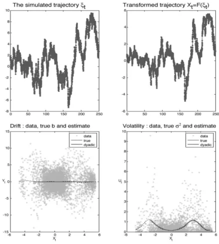
5.7.1 Examples of diffusions Family 1
First, we consider (5.1) with
b(x) =−✓x, σ(x) = c(1 + x2)1/2.
Standard computations of the scale and speed densities show that the model is positive recurrent for ✓+ c2/2 > 0. In this case, its stationary distribution has
density
⇡(x)/ 1 (1 + x2)1+✓/c2.
IfX0 = ⌘ has distribution ⇡(x)dx, then, setting ⌫ = 1 + 2✓/c2, ⌫1/2⌘ has
Student distributiont(⌫). This distribution satisfies the moment condition [A6] for2✓/c2> 7. See Figure 5.1 for the estimation of b and σ2in this case.
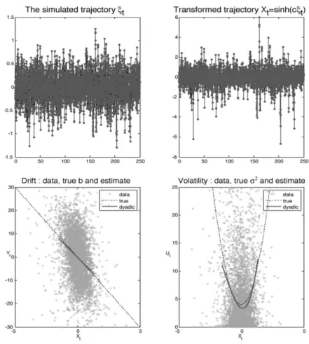
Then, we considerF1(x) = R0x1/(c(1 + x2)1/2dx = arg sinh(x)/c. By the
Itˆo formula, ⇠t = F1(Xt) is solution of a stochastic differential equation with
σ(⇠) = 1 and
Figure 5.1 First example:dXt=−θXtdt+, cp1 + Xt2dWt,n = 5000, ∆ = 1/20,
θ = 2, c = 1, dotted line: true function, full line: estimated function.
Assumptions [A1] – [A3] and [A5] hold for(⇠t) with ⇠0 = F1(X0).
More-over,(⇠t) satisfies the conditions of Proposition 1 in Pardoux and Veretennikov
(2001) implying that(⇠t) is exponentially β-mixing and has moments of any
order. Hence, [A4] and [A6] hold. See Figure 5.2 for the estimation of b and σ2in this case.
Since Xt= F1−1(⇠t), this process is also β-mixing. It satisfies all assumptions
Figure 5.2 Second example:dξt=−(θ/c + c/2) tanh(cξt) + dWt,n = 5000, ∆ =
1/20, θ = 6, c = 2, dotted line: true function, full line: estimated function.
Family 2
For the second family of models, we consider a process(⇠t) with diffusion
coefficient σ(⇠) = 1 and drift
b(⇠) =−✓ ⇠
(1 + c2⇠2)1/2, (5.40)
(see Barndorff-Nielsen (1978)). The model is positive recurrent on R for ✓> 0. Its stationary distribution is a hyperbolic distribution given by
⇡(⇠)d⇠/ exp(−2✓ c2(1 + c
2⇠2)1/2).
Assumptions [A1] – [A3], [A5] – [A6] hold for this model. For [A4], we apply Proposition 1 of Pardoux and Veretennikov (2001).
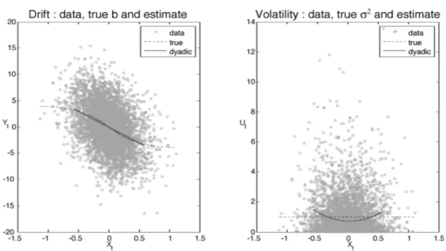
Next, we considerXt = F2(⇠t) = arg sinh(c⇠t) which satisfies a stochastic
differential equation with coefficients: b(x) =− ✓ ✓+ c 2 2 cosh(x) ◆ sinh(x) cosh2(x), σ(x) = c cosh(x).
The process(Xt) is exponentially β-mixing as (⇠t). The diffusion coefficient
σ(x) has an upper bound. See Figure 5.3 for the estimation of b and σ2in this
case.
Figure 5.3 Third example,dXt=− [θ + c2/(2 cosh(Xt))] (sinh(Xt)/ cosh2(Xt))dt
+(c/ cosh(Xt))dWt,n = 5000, ∆ = 1/20, θ = 3, c = 2, dotted line: true function,
full line: estimated function.
we consider Xt= G(⇠t) = arg sinh(⇠t− 5) + arg sinh(⇠t+ 5). The function
G(.) is invertible and its inverse has the following explicit expression, G−1(x) = 1
21/2 sinh(x)
⇥
49 sinh2(x) + 100 + cosh(x)(sinh2(x)− 100)⇤1/2. The diffusion coefficient of(Xt) is given by
σ(x) = 1
(1 + (G−1(x)− 5)2)1/2 +
1
The drift is given by G0(G−1(x))b(G−1(x)) + 1
2G00(G−1(x)) with b given in
(5.40). See Figure 5.4 for the estimation of b and σ2in this case.
Figure 5.4 Fourth example, the two-bumps diffusion coefficientXt = G(ξt), dξt =
−θξt/p1 + c2ξ2tdt + dWt,G(x) = arg sinh(x− 5) + arg sinh(x + 5), n = 5000,
∆ = 1/20, θ = 1, c = 10, dotted line: true function, full line: estimated function.
Family 3
Consider Yta stationary Ornstein-Uhlenbeck process given by dYt=−✓Ytdt+
can be evaluated using the exact formula (5.2). This gives a direct proof of (5.3).
Proposition 5.14 Theβ-mixing coefficient of(Yt) satisfies
βY(t)
exp (−✓t) 2(1− exp (−✓t)).
Proof. We use the expansion of the transition densitypt(x, y) of (Yt) in terms
of the sequence of eigenvalues and eigenfunctions of the infinitesimal genera-torLf (y) = σ2
2f00(y)− ✓yf0(y). For this, we refer e.g. to Karlin and Taylor
(1981, p.333). To simplify notations, we assume that σ2/2✓ = 1 so that the stationary distribution of(Yt) is ⇡(y)dy =N (0, 1). Let us now consider the
n-th Hermite polynomial given, for n = 0, 1, . . ., by: Hn(x) = (−1)n p n! exp (x 2/2) dn dxn[exp (−x 2/2)].
As defined above, this sequence is an orthonormal basis ofL2(⇡) and satisfies,
for alln≥ 0, LHn = −n✓Hn, i.e.,Hnis the eigenfunction associated with
the eigenvalue−n✓ of L. This gives the following expansion: pt(x, y) = ⇡(y)
+1
X
n=0
exp (−n✓t)Hn(x)Hn(y).
SinceH0(x) = 1 and the HnhaveL2(⇡)-norm equal to 1, we get
kpt(x, y)dy− ⇡(y)dykT V = 1 2 Z R|p t(x, y)− ⇡(y)|dy 12 +1 X n=1 exp (−n✓t)|Hn(x)| Z R|H n(y)|⇡(y)dy 12 +1 X n=1 exp (−n✓t)|Hn(x)|.
Integrating w.r.t. ⇡(x)dx and repeating the same tool, we obtain:
βY(t) 1 2 +1 X n=1 exp (−n✓t) = exp (−✓t) 2(1− exp (−✓t)).
The interest of this proof is that it can be mimicked for all models for which the infinitesimal generator has a discrete spectrum with explicit eigenfunctions and eigenvalues.
Now, we consider Xt = tanh(Yt). By the Itˆo formula, we get that (Xt) has coefficients b(x) =−(1 − x2) c2x +✓ 2ln ✓ 1 + x 1− x ◆$ , σ(x) = c(1− x2).
Assumptions [A1] – [A6] are satisfied for(Xt).
Finally, we consider dXt = dc2 4 − ✓Xt $ dt + cpXtdWt.
Withd ≥ 2 integer, (Xt) has the distribution ofPdi=1Yi,t2 where(Yi,t) are
i.i.d. Ornstein-Uhlenbeck processes as above. The process (Xt) satisfies all
assumptions except that its diffusion coefficient is not bounded.
5.7.2 Calibrating the penalties
It is not easy to calibrate the penalties. The method is studied in full details in Comte and Rozenholc (2004). Implementation with [DP] is done on the above examples in Comte et al. (2007) and for [GP] in Comte et al. (2006). We only give here a brief description.
For collection [GP], the drift penalty(i = 1) and the diffusion penalty (i = 2) are given by 2ˆs 2 i n 0 @d − 1 + ln✓ dmax− 1 d− 1 ◆ + ln2.5(d) + d X j=1 (rj+ ln2.5(rj+ 1)) 1 A .
Moreover,dmax = [n∆/ ln1.5(n)], rmax = 5. The constants and ˜ in both
drift and diffusion penalties have been set equal to 2. The termsˆ2
1 replaces
σ21/∆ for the estimation of b and ˆs22replaces σ41for the estimation of σ2. Let
us first explain howsˆ2
2is obtained. We run once the estimation algorithm of
σ2 with a preliminary penalty wheresˆ2
2 is taken equal to2 maxm(˘γn(ˆσm2)).
This gives a preliminary estimator ˜σ20. Now, we take ˆs2 equal to twice the
99.5%-quantile ofσ˜2
0. The use of the quantile here is to avoid extreme values.
We getσ˜2. We use this estimate and setˆs2
1= max1kn(˜σ2(Xk∆))/∆ for the
penalty ofb. In all the examples, parameters have been chosen in the admissible range of ergodicity. The sample sizen = 5000 and the step ∆ = 1/20 are in accordance with the asymptotic context (greatn’s and small ∆’s).
5.8 Bibliographical remarks
Non-parametric estimation of the coefficients of diffusion processes has been widely investigated in the last decades. There are two first reference papers which are only devoted to drift estimation. One is by Banon (1978), who uses a spectral approach and a continuous time observation of the sample path. The other one is by Tuan (1981) who constructs and studies kernel estimators of the drift based on a continuous time observation of the sample path and also on a discrete observation of the sample path for an ergodic diffusion process. More recently, several authors have considered drift estimation based on a con-tinuous time observation of the sample path for ergodic models. Asymptotic results are given as the length of the observation time interval tends to infinity (Prakasa Rao (2010), Spokoiny (2000), Kutoyants (2004) or Dalalyan (2005)). Discrete sampling of observations has also been investigated, with different asymptotic frameworks, implying different statistical strategies. It is now clas-sical to distinguish between low-frequency and high-frequency data. In the for-mer case, observations are taken at regularly spaced instants with fixed sam-pling interval∆ and the asymptotic framework is that the number of obser-vations tends to infinity. Then, only ergodic models are usually considered. Parametric estimation in this context has been studied by Bibby and Sørensen (1995), Kessler and Sørensen (1999), see also Bibby, Jacobsen, and Sørensen (2009). A non-parametric approach using spectral methods is investigated in Gobet, Hoffmann, and Reiß (2004), where non-standard non-parametric rates are exhibited.
In high-frequency data, the sampling interval∆ = ∆n between two
succes-sive observations is assumed to tend to zero as the number of observations n tends to infinity. Taking∆n = 1/n, so that the length of the observation time
intervaln∆n= 1 is fixed, can only lead to estimating the diffusion coefficient
consistently with no need of ergodicity assumptions. This is done by Hoffmann (1999) who generalizes results by Jacod (2000), Florens-Zmirou (1993) and Genon-Catalot, Lar´edo, and Picard (1992).
Now, estimating both drift and diffusion coefficients requires that the sampling interval∆n tends to zero whilen∆n tends to infinity. For ergodic diffusion
models, Hoffmann (1999) proposes non-parametric estimators using projec-tions on wavelet bases together with adaptive procedures. He exhibits mini-max rates and shows that his estimators automatically reach these optimal rates up to logarithmic factors. Hence, Hoffmann’s paper gives the benchmark for studying non-parametric estimation in this framework and assumptions. Nev-ertheless, Hoffmann’s estimators are based on computations of some random times which make them difficult to implement.
asymptotic framework but with nonstationary diffusion processes: they study kernel estimators using local time estimations and random normalization.
5.9 Appendix. Proof of Proposition 5.13
The proof relies on the following Lemma (Lemma 9 in Barron et al. (1999)): Lemma 5.15 Letµ be a positive measure on[0, 1]. Let ( λ)λ2Λbe a finite
orthonormal system in L2\ L1(µ) with|Λ| = D and ¯S be the linear span of
{ λ}. Let ¯ r = p1 Dsupβ6=0 kPλ2Λβλ λk1 |β|1 .
For any positiveδ, one can find a countable setT ⇢ ¯S and a mapping p from ¯
S to T with the following properties: • for any ball B with radius σ ≥ 5δ,
|T \ B| (B0σ/δ)D with B0< 5. • ku − p(u)kµ δ for all u in ¯S, and
sup
u2p−1(t)ku − tk1 ¯rδ, for all t in T.
To use this lemma, the main difficulty is often to evaluate¯r in the different contexts. In our problem, the measureµ is ⇡. We consider a collection of mod-els(Sm)m2Mn which can be [DP] or [GP]. Recall thatB
⇡
m,m0(0, 1) = {t 2
Sm+ Sm0,ktk⇡ = 1}. We have to compute ¯r = ¯rm,m0 corresponding to
¯
S = Sm+ Sm0. We denote byD(m, m0) = dim(Sm+ Sm0).
Collection [DP]–Sm+ Sm0 = Smax(m,m0),D(m, m0) = max(Dm, Dm0), an
orthonormal L2(⇡)-basis ( λ)λ2Λ(m,m0)can be built by orthonormalisation,
on each sub-interval, of('λ)λ2Λ(m,m0). Then
sup β6=0 kPλ2Λ(m,m0)βλ λk1 |β|1 k X λ2Λ(m,m0) | λ|k1 (rmax+ 1) sup λ2Λ(m,m0)k λk1 (rmax+ 1)3/2 p D(m, m0) sup λ2Λ(m,m0)k λk (rmax+ 1)3/2 p D(m, m0) sup λ2Λ(m,m0)k λk⇡ /p⇡0 (rmax+ 1)3/2 p D(m, m0)/⇡0.
Thus herer¯m,m0 (rmax+ 1)3/2/p⇡0.
Collection [GP]– Here we have¯rm,m0 [(rmax+ 1)pNn]/
p
D(m, m0)⇡0.
We now prove Proposition 5.13. We apply Lemma 5.15 to the linear space Sm+ Sm0 of dimensionD(m, m0) and norm connection measured by ¯rm,m0
bounded above. We consider δk-nets,Tk = Tδk \ B
⇡
m,m0(0, 1), with δk =
δ02−kwith δ0 1/5, to be chosen later and we set
Hk= ln(|Tk|) D(m, m0) ln(5/δk) = D(m, m0)[k ln(2) + ln(5/δ0)].
(5.41) Given some point u 2 B⇡
m,m0(0, 1), we can find a sequence {uk}k≥0 with
uk2 Tksuch thatku − ukk2⇡ δk2andku − ukk1 ¯rm,m0δk. Thus we have
the following decomposition that holds for anyu2 B⇡
m,m0(0, 1), u = u0+ 1 X k=1 (uk− uk−1).
Clearlyku0k⇡ 1, ku0k1 ¯r(m,m0)and for allk ≥ 1, kuk − uk−1k2⇡
2(δ2
k+ δk2−1) = 5δ2k−1/2 andkuk− uk−1k1 3¯r(m,m0)δk−1/2. In the sequel
we denote by Pn(.) the measure P(.\ Ωn), see (5.24), (actually only the
in-equalityktk2n 32ktk⇡2 holding for anyt2 Sm+ Sm0is required).
Let(⌘k)k≥0be a sequence of positive numbers that will be chosen later on and
⌘ such that ⌘0+Pk≥1⌘k ⌘. Recall that ˘⌫n(1)is defined by (5.27) – (5.32) –
(5.33). We have IPn " sup u2Bπ m,m0(0,1) ˘ ⌫n(1)(u) > ⌘ # = IPn " 9(uk)k2N2 Y k2N Tk/ ˘ ⌫n(1)(u0) + +1 X k=1 ˘ ⌫n(1)(uk− uk−1) > ⌘0+ X k≥1 ⌘k # IP1+ IP2 where IP1 = X u02T0 IPn(˘⌫n(1)(u0) > ⌘0), IP2 = 1 X k=1 X uk−12Tk−1 uk2Tk IPn(˘⌫n(1)(uk− uk−1) > ⌘k).
Then using inequality (5.37) of Lemma 5.12 and (5.41), we straightforwardly infer that IP1 exp(H0− Cnx0) and IP2Pk≥1exp(Hk−1+ Hk− Cnxk)
if we choose ⇢ ⌘0= σ21( p 3x0+ ¯r(m,m0)x0) ⌘k = (σ21/ p 2)δk−1(p15xk+ 3¯r(m,m0)xk).
Fix ⌧ > 0 and choose x0such that
Cnx0= H0+ Lm0Dm0+ ⌧
and fork≥ 1, xksuch that
Cnxk = Hk−1+ Hk+ kDm0+ Lm0Dm0+ ⌧. IfDm0 ≥ 1, we infer that IPn sup t2Bπ m,m0(0,1) ˘ ⌫n(1)(t) > ⌘0+ X k≥1 ⌘k ! e−Lm0Dm0−⌧ 1 + 1 X k=1 e−kDm0 ! 1.6e−Lm0Dm0−⌧.
Now, it remains to computePk≥0⌘k. We note thatPk=01 δk =P1k=0kδk =
2δ0. This implies x0+ 1 X k=1 δk−1xk " ln(5/δ0) + δ0 1 X k=1 2−(k−1)[(2k− 1) ln(2) + 2 ln(5/δ0) + k] # ⇥D(m, mnC 0) + 1 + δ0 X k≥1 2−(k−1) ! ✓ Lm0Dm0 nC + ⌧ nC ◆ a(δ0) D(m, m0) n + ( 1 + 2δ0 C )( Lm0Dm0 n + ⌧ n), (5.42)
where Ca(δ0) = ln(5/δ0) + δ0(4 ln(5/δ0) + 6 ln(2) + 4). This leads to 1 X k=0 ⌘k !2 σ 4 1 2 " p 2(p3x0+ +¯rm,m0x0)+ 1 X k=1 δk−1(p15xk+ 3¯rm,m0xk) #2 σ 4 1 2 " p 6x0+ 1 X k=1 δk−1p15xk ! + ¯rm,m0 p 2x0+ 3 1 X k=1 δk−1xk !#2 15σ4 1 2 4 px0+ 1 X k=1 δk−1pxk !2 + ¯r2 m,m0 x0+ 1 X k=1 δk−1xk !23 5 15σ41 " 1 + 1 X k=1 δk−1 ! x0+ 1 X k=1 δk−1xk ! +¯r2 m,m0 x0+ 1 X k=1 δk−1xk !23 5 .
Now, fix δ0 1/5 (say, δ0= 1/10) and use the bound (5.42). The bound for
(P+1k=0⌘k)2is less than a quantity proportional to
σ41 " D(m, m0) n + Lm0Dm0 n + ¯r 2 m,m0 ✓ D(m, m0) n + Lm0Dm0 n ◆2 + ⌧ n+ ¯r 2 m,m0 ⌧2 n2 $ .
Now in the case of collection [DP], we have Lm = 1, ¯rm,m0 is bounded
uniformly with respect to m and m0 and (D(m, m0)/n)2 (N
n/n)2
∆2/ ln4(n) with N
n n∆/ ln2(n). Thus the bound for (P⌘k)2reduces to
C0σ14 D(m, m0) n + (1 + rmax) 3∆2/⇡ 0+ ⌧ n+ ¯r 2 m,m0 ⌧2 n2 $ .
Next, for collection [GP], we use that Lm c ln(n), ¯r2m,m0 (rmax +
1)3N
n/(⇡0D(m, m0)) and Nn n∆/ ln2(n) to obtain the bound
¯ r2m,m0 ✓ D(m, m0) n + Lm0Dm0 n ◆2 (rmax+ 1)3 Nn ⇡0D(m, m0) D(m, m0)2 n2 (1 + ln(n)) 2 (rmax+ 1)3 NnD(m, m0) ⇡0n2 (1 + ln(n))2 (rmax+ 1)3 N2 n ⇡0n2 (1 + ln(n))2 2(r max+ 1)3∆2/⇡0.
Thus, the bound for(P⌘k)2is proportional to
σ41 D(m, m0) n + Lm0Dm0 n + 2(rmax+ 1) 3∆2/⇡ 0+ ⌧ n+ ¯r 2 m,m0 ⌧2 n2 $ .
This term definesp(m, m˜ 0) as given in Proposition 5.13.
We obtain, forK = (rmax+ 1)3/⇡0,
IPn " sup u2Bπ m,m0(0,1) [˘⌫n(1)(u)]2> σ14 ✓D m+ Dm0(1 + Lm0) n +K∆2+ 2(⌧ n_ 2¯r 2 m,m0 ⌧2 n2) ◆$ IPn " sup u2Bπ m,m0(0,1) [˘⌫n(1)(u)]2> ⌘2 # 2IPn " sup u2Bπ m,m0(0,1) ˘ ⌫n(1)(u) > ⌘ # 3.2e−Lm0Dm0−⌧
so that, reminding that ˘Gm(m0) is defined by (5.39), E ✓ ˘ G2m(m0)− σ41Dm+ Dm0(1 + Lm0) n + K∆ 2 ◆ + 1Ωn $ Z 1 0 Pn ✓ ˘ G2m(m0) > σ41 Dm+ Dm0(1 + Lm0) n + K∆ 2+ ⌧◆ d⌧ e−Lm0Dm0 Z 1 2σ4 1/¯r(m,m0 )2 e−n⌧/(2σ41)d⌧ + Z 2σ4 1/¯rm,m02 0 e−np⌧ /(2p¯rm,m0σ21)d⌧ ! e−Lm0Dm02σ 4 1 n Z 1 0 e−vdv+2¯r 2 m,m0 n Z 1 0 e−pvdv ! e−Lm0Dm02σ 4 1 n (1 + 4¯rm,m2 0 n ) 0e−Lm0Dm0σ 4 1 n which ends the proof. 2
References
Abramowitz, M., & Stegun, A. (1972). Handbook of mathematical functions
with formulas, graphs, and mathematical tables. Wiley, New York. Bandi, F. M., & Phillips, P. C. B. (2003). Fully nonparametric estimation of
scalar diffusion models. Econometrica, 71, 241–283.
Banon, G. (1978). Nonparametric identification for diffusion processes. SIAM
J. Control Optim., 16, 380–395.
Baraud, Y., Comte, F., & Viennet, G. (2001a). Adaptive estimation in autore-gression or β-mixing reautore-gression via model selection. Ann. Statist., 29, 839–875.
Baraud, Y., Comte, F., & Viennet, G. (2001b). Model selection for (auto)-regression with dependent data. ESAIM Probab. Statist., 5, 33–49. Barlow, M. T., & Yor, M. (1982). Semimartingale inequalities via the
Garsia-Rodemich-Rumsey lemma, and applications to local times. J. Funct.
Anal., 49, 198–229.
Barndorff-Nielsen, O. E. (1978). Hyperbolic distributions and distributions on hyperbolae. Scand. J. Statist., 5, 151–157.
Barron, A. R., Birg´e, L., & Massart, P. (1999). Risk bounds for model selection via penalization. Probab. Theory Related Fields, 113, 301–413. Beskos, A., Papaspiliopoulos, O., & Roberts, G. O. (2006). Retrospective
exact simulation of diffusion sample paths with applications. Bernoulli,
12, 1077–1098.
Beskos, A., & Roberts, G. O. (2005). Exact simulation of diffusions. Ann.
Appl. Probab., 15, 2422–2444.
Bibby, B. M., Jacobsen, M., & Sørensen, M. (2009). Estimating functions for discretely sampled diffusion-type models. In Y. A¨ıt-Sahalia & L. Hansen (Eds.), Handbook of Financial Econometrics (pp. 203–268). North Hol-land, Oxford.
Bibby, B. M., & Sørensen, M. (1995). Martingale estimation functions for discretely observed diffusion processes. Bernoulli, 1, 17–39.
Birg´e, L., & Massart, P. (1998). Minimum contrast estimators on sieves: ex-ponential bounds and rates of convergence. Bernoulli, 4, 329–375. Comte, F. (2001). Adaptive estimation of the spectrum of a stationary Gaussian
sequence. Bernoulli, 7, 267–298.
Comte, F., Genon-Catalot, V., & Rozenholc, Y. (2006). Nonparametric
esti-mation of a discretely observed integrated diffusion model.(Tech. Rep.). MAP 5, Math´ematiques Appliqu´ees - Paris 5, UMR CNRS 8145. Comte, F., Genon-Catalot, V., & Rozenholc, Y. (2007). Penalized
nonpara-metric mean square estimation of the coefficients of diffusion processes.
Bernoulli, 13, 514–543.
Comte, F., & Rozenholc, Y. (2002). Adaptive estimation of mean and volatil-ity functions in (auto-)regressive models. Stochastic Process. Appl., 97, 111–145.
Comte, F., & Rozenholc, Y. (2004). A new algorithm for fixed design regres-sion and denoising. Ann. Inst. Statist. Math., 56, 449–473.
Dalalyan, A. (2005). Sharp adaptive estimation of the drift function for ergodic diffusions. Ann. Statist., 33, 2507–2528.
DeVore, R. A., & Lorentz, G. G. (1993). Constructive Approximation. Berlin: Springer.
Florens-Zmirou, D. (1993). On estimating the diffusion coefficient from dis-crete observations. J. Appl. Probab., 30, 790–804.
Genon-Catalot, V., Jeantheau, T., & Lar´edo, C. (2000). Stochastic volatility models as hidden markov models and statistical applications. Bernoulli,
6, 1051–1079.
Genon-Catalot, V., Lar´edo, C., & Picard, D. (1992). Nonparametric estimation of the diffusion coefficient by wavelet methods. Scand. J. Statist., 19, 319–335.
Gobet, E., Hoffmann, M., & Reiß, M. (2004). Nonparametric estimation of scalar diffusions based on low frequency data. Ann. Statist., 32, 2223– 2253.
Hoffmann, M. (1999). Adaptive estimation in diffusion processes. Stochastic
Process. Appl., 79, 135–163.
Jacod, J. (2000). Non-parametric kernel estimation of the coefficient of a diffusion. Scand. J. Statist., 27, 83–96.
Karlin, S., & Taylor, H. M. (1981). A Second Course in Stochastic Processes. New York: Academic Press.
Kessler, M., & Sørensen, M. (1999). Estimating equations based on eigenfunc-tions for a discretely observed diffusion process. Bernoulli, 5, 299–314. Kutoyants, Y. A. (2004). Statistical Inference for Ergodic Diffusion Processes.
London: Springer.
Pardoux, E., & Veretennikov, A. Y. (2001). On the Poisson equation and diffusion approximation. I. Ann. Probab., 29, 1061–1085.
Prakasa Rao, B. L. S. (2010). Statistical Inference for Fractional Diffusion
Processes. Chichester: Wiley.
Spokoiny, V. G. (2000). Adaptive drift estimation for nonparametric diffusion model. Ann. Statist., 28, 815–836.
Tuan, P. D. (1981). Nonparametric estimation of the drift coefficient in the diffusion equation. Math. Operationsforsch. Statist., Ser. Statistics, 12, 61–73.
![Figure 5.3 Third example, dX t = − [θ + c 2 /(2 cosh(X t ))] (sinh(X t )/ cosh 2 (X t ))dt +(c/ cosh(X t ))dW t , n = 5000, ∆ = 1/20, θ = 3, c = 2, dotted line: true function, full line: estimated function.](https://thumb-eu.123doks.com/thumbv2/123doknet/15015896.681106/28.892.229.666.232.724/figure-example-cosh-sinh-dotted-function-estimated-function.webp)