GJI
Geo
dynamics
and
tectonics
Three-dimensional P-wave velocity structure on the shallow part
of the Central Costa Rican Pacific margin from local earthquake
tomography using off- and onshore networks
I. G. Arroyo,
1S. Husen,
2E. R. Flueh,
1J. Gossler,
1E. Kissling
2and G. E. Alvarado
31Leibniz Institute for Marine Science (IfM-Geomar) and SFB574, Kiel, Germany. E-mail: [email protected] 2Swiss Federal Institute of Technology Zurich, ETH Hoenggerberg, Zurich, Switzerland
3Instituto Costarricense de Electricidad (ICE) and Universidad de Costa Rica, San Jos´e, Costa Rica (Red Sismol´ogica Nacional-RSN)
Accepted 2009 July 21. Received 2009 June 21; in original form 2008 April 25
S U M M A R Y
The Central Costa Rican Pacific margin is characterized by a high-seismicity rate, coincident with the subduction of rough-relief ocean floor and has generated earthquakes with magnitude up to seven in the past. We inverted selected P-wave traveltimes from earthquakes recorded by a combined on- and offshore seismological array deployed during 6 months in the area, simultaneously determining hypocentres and the 3-D tomographic velocity structure on the shallow part of the subduction zone (<70 km). The results reflect the complexity associated to subduction of ocean-floor morphology and the transition from normal to thickened subducting oceanic crust. The subducting slab is imaged as a high-velocity perturbation with a band of low velocities (LVB) on top encompassing the intraslab seismicity deeper than∼30 km. The LVB is locally thickened by the presence of at least two subducted seamounts beneath the margin wedge. There is a general eastward widening of the LVB over a relatively short distance, closely coinciding with the onset of an inverted forearc basin onshore and the appearance of an aseismic low-velocity anomaly beneath the inner forearc. The latter coincides spatially with an area of the subaerial forearc where differential uplift of blocks has been described, suggesting tectonic underplating of eroded material against the base of the upper plate crust. Alternatively, the low velocities could be induced by an accumulation of upward migrating fluids. Other observed velocity perturbations are attributed to several processes taking place at different depths, such as slab hydration through outer rise faulting, tectonic erosion and slab dehydration.
Key words: Seismic tomography; Subduction zone processes; Continental margins:
conver-gent; Crustal structure.
1 I N T R O D U C T I O N
The convergent margin along the Middle America Trench (MAT) off Costa Rica and Nicaragua has been the focus during the first stage of the project SFB574 ‘Volatiles and Fluids in Subduction Zones’, which aims to better understand the processes involved in the exchange of fluids in erosional convergent margins. The diver-sity in structure and morphology of the incoming Cocos Plate and its associated effects on the structure of the margin, such as variations in the subduction angle, depth of the Wadati-Benioff seismicity, deformation style, plate coupling and magmatic composition along the volcanic front, confer special interest to the area.
Being a direct response to the dynamics and structure of subduc-tion zones, their seismicity and velocity structure provide valuable insights into the processes taking place in these regions, where more than 80 per cent of the seismic energy of the Earth is released. Local earthquake tomography (LET) is one of the most powerful methods
to obtain precise local earthquake locations and detailed knowledge of the 3-D velocity field, as proved in this (Protti et al. 1996; Husen
et al. 2003a; DeShon et al. 2006) and other subduction zones.
The Central Pacific region of Costa Rica displays a very high-seismicity rate, coinciding with the subduction of rough-relief ocean floor, which includes seamounts and plateaus (Fig. 1). The area has generated earthquakes with magnitude up to seven in the past, most recently a Mw6.9 event in 1999 and a Mw6.4 in 2002. As part of the SFB574, an ‘amphibious’ network, consisting of land and ocean-bottom stations, was installed in the area for a period of 6 months. Since commonly the trench and forearc regions of subduction zones are located offshore, the availability of ocean-bottom hydrophones offers an excellent opportunity to study the shallower part of the margin. This makes the determination of high-quality hypocentre locations possible for the first time in this area, where the quality and completeness of the seismic catalogues from the two permanent countrywide networks is impaired by the lack of coverage offshore.
828 I. G. Arroyo et al.
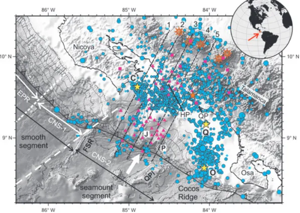
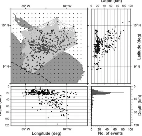
Figure 1. Setting of the Jac´o seismological experiment in the Central Pacific margin of Costa Rica. The network (triangles) consisted of land and ocean-bottom stations that operated from 2002 April to October; additional readings from land stations of the permanent network RSN (red squares) improved the coverage. Total recorded seismicity during the experiment is shown (blue circles). Dashed lines denote the location of vertical cross-sections shown in Fig. 14. Bathymetry (exaggerated), including contours every 500 m, and main tectonic segments after von Huene et al. (2000) and Barckhausen et al. (2001), respectively. Cocos Plate oceanic crust was formed at the East Pacific Rise (EPR) and at the Cocos-Nazca Spreading Center (CNS). Cocos Plate motion azimuth (thick white arrow) from DeMets et al. (1994). Radiating circles denote Holocene volcanoes in central Costa Rica. Yellow stars represent the epicentres of recent large earthquakes associated to subduction of bathymetric highs: C: 1990 Mw7.0 C´obano (Husen et al. 2002), Q: 1999 Mw6.9 Quepos (location from Universidad
Nacional de Costa Rica) and O: 2002 Mw6.4 Osa (preliminary location from Jac´o and RSN networks combined). Orange star: upper-plate, 2004 Mw 6.4
Damas earthquake (Pacheco et al. 2006). HP: Herradura Promontory, QP: Quepos Promontory, FSR: Fisher Seamount and Ridge, QPl: Quepos Plateau, J: Jac´o Scar and P: Parrita Scar.
The main goals of the experiment include the characterization of the seismicity in this portion of the margin and its correlation with the tectonic and velocity structure, with emphasis on the seis-mogenic zone, that is, the zone were the overriding and subducting plates are coupled. Foregoing studies lacked the coverage necessary to define the limits of the interplate seismicity, which are essential for the definition of the seismogenic zone and the process control-ling its extent. The Costa Rican Central Pacific margin provides also the possibility of studying the effects of seamounts at differ-ent stages of subduction on seismicity, velocity structure and the seismogenic zone. Moreover, with most of the seismogenic zone re-search carried out to date in accretionary margins, the results of this and similar experiments in the area could augment our understand-ing of the processes takunderstand-ing place in tectonically erosive margins, as well as the characteristics common to both margin types.
Furthermore, the Costa Rican margin has been the target of sev-eral controlled-source seismology (CSS) campaigns for more than 30 yr. In addition to swath bathymetry, gravimetric and magnetic surveys, heat flow measurements and drilling projects, an extensive assemblage of modern near-vertical and wide-angle reflection lines has been collected in the area, largely offshore, specially since the 1990s. In this study, we collect information from CSS lines available in the area resolvable with LET and incorporate it indirectly into the inversion process, aiming to preserve the strength of each method.
Instead of including shots into the inversion, we rather adjust the reference model with information from CSS, which also facilitates greatly the interpretation of observed tomographic anomalies.
We present here the results of the simultaneous inversion of Vp and hypocentral parameters, with focus on the 3-D velocity structure of the Central Pacific margin of Costa Rica. The LET images the subducting slab as a high-velocity feature topped by a continuous band of low velocities from the trench down to∼70 km, where the resolution of our model ends. This low-velocity band (LVB) broadens downdip and, more conspicuously, towards the east. We interpret these and other results as the outcome of slab dehydration, subduction erosion, tectonic underplating or fluid accumulation at the base of the overlying plate, and the subduction of thickened oceanic crust and accompanying bathymetric highs.
2 T E C T O N I C F R A M E W O R K
Costa Rica is located on the western margin of the Caribbean Plate, where subduction of the Cocos Plate takes place along the MAT with a convergence direction of 32◦ and subduction rates varying from 8.3 cm yr−1 in Northwestern Costa Rica to 9.0 cm yr−1 in the southeast (DeMets et al. 1994). The high seismic activity in the area is generated by the subduction process, crustal deformation and magmatic activity along the volcanic front.
The lithosphere of the Cocos Plate subducting at the MAT to-day has been created at the fast-spreading East Pacific Rise (EPR) and at the present, slow-spreading Cocos-Nazca Spreading Cen-ter (CNS) and its precursors. The CNS segment has been partially modified by Galapagos hotspot magmatism. The boundary between the oceanic crusts formed at both centres is located offshore the Nicoya Peninsula (Fig. 1). The crust formed at the EPR is 24 Ma at the MAT, while the crust offshore Central and Southeastern Costa Rica has ages ranging from 19 to 15 Ma (Werner et al. 1999; Barckhausen et al. 2001), respectively. The thickness of the Cocos Plate crust varies from 5 to 7 km offshore Nicoya (Sallar`es et al. 2001; Walther & Flueh 2002), to 6–8 km at the seamount domain (Ye et al. 1996; Walther 2003) and reaches up to 19–21 km be-neath the Cocos Ridge (Walther 2003; Sallar`es et al. 2003). Three domains have been identified by von Huene et al. (1995, 2000) in the highly variable morphotectonics displayed by the Cocos Plate offshore Costa Rica (Fig. 1). Facing the Nicoya Peninsula, the sub-ducting seafloor has a smooth relief, whereas to the southeast the Cocos Ridge stands 2 km high over the surrounding ocean floor. The segment in between, the area of this study, stretches from the Fisher Seamount and Ridge until the Quepos Plateau, and it is 40 per cent covered by seamounts. Substantial deformation of the continental slope in the form of deep furrows and domes indicates seamount subduction and there is evidence that they remain attached to the subducting plate to depths of∼25 km, eventually causing coastal uplift (Fisher et al. 1998; Gardner et al. 2001) and large earthquakes (Husen et al. 2002). The seamounts have a Galapagos geochemistry, being 13–14.5 Ma adjacent to the margin (Werner et al. 1999).
High-quality seismic lines, high-resolution bathymetry and ocean drilling allow the conclusion that the Middle American convergent margin has been tectonically erosive since the Middle Miocene (Ranero & von Huene 2000; von Huene et al. 2000; Vanucchi
et al. 2001). Basal tectonic erosion offshore Costa Rica causes
mass removal, and subsequent crustal thinning and margin subsi-dence, at high non-steady rates ranging from long-term∼45 to 107– 123 km3Ma−1km−1during the last 6.5 Ma (Vannucchi et al. 2003). Ranero & von Huene (2000) identified two specific mechanisms of subduction erosion along the Middle American margin: erosion by seamount tunnelling and removal of large rock lenses of a distending upper plate.
The along-strike segmentation of the Cocos Plate appears to have a strong tectonic effect on the upper plate. Significant variations in the subduction angle, the nature of the incoming plate and magmatic composition along the volcanic arc occur along this margin (Carr & Stoiber 1990; Protti et al. 1995a; von Huene et al. 2000; Husen
et al. 2003a). In Southeastern Costa Rica, cessation of volcanic
activity and accelerated uplift of the Talamanca Cordillera since 3.5 Ma have been attributed to the northwest-to-southeast shallow-ing of the slab as a response to the subduction of the Cocos Ridge solely or, more recently, first to the subduction of the Coiba Ridge and the passage of the Cocos–Nazca–Caribbean triple junction and the subsequent subduction of Cocos Ridge (MacMillan et al. 2004). This slab shallowing, together with trench retreat by forearc ero-sion, have been invoked to explain the northeastward migration of the volcanic front in Central Costa Rica from its position during the Miocene–Pliocene to its current location (Marshall et al. 2003; Fig. 1).
The basic structural configuration of the margin offshore Costa Rica and Nicaragua (Hinz et al. 1996; Kimura et al. 1997; Ranero
et al. 2000) consists of a margin wedge composed of the same ocean
igneous and associated sedimentary rocks that outcrop at several spots along the coast in Costa Rica, covered by slope sediments,
un-derthrust by trench sediments and gouge made of upper-plate mate-rial and faced by a small frontal prism. This basic structure is altered in places where seamounts are in the first stages of subduction, but it is a short-term damage: after∼0.5 Ma the morphology and struc-ture of the margin become nearly undistinguishable from places were no seamount subducts (von Huene et al. 2000). The oceanic assemblages cropping out at the Pacific coastal areas include a pre-Campanian oceanic plateau association in the Nicoya Peninsula and in the outer Herradura Promontory; an accreted oceanic island of Maastrichtian to lower Eocene age which forms the main edifice of the Herradura Promontory; and the Quepos Promontory, formed by the accretion of an Upper Cretaceous–Paleocene seamount (Hauff
et al. 2000; Denyer et al. 2006).
Coinciding with the seamount segment, the Central Pacific region of Costa Rica shows the highest seismicity rate along the south-ern section of the MAT. The absence of very large earthquakes
( ˙Mw> 7.5) and the high rate of small earthquakes define this part
of the subduction zone as seismically decoupled (Protti et al. 1994), while coupling increases to the northwest and to the southeast. Sev-eral studies have found evidence of the relationship between the subduction of bathymetric highs and the generation of large sub-duction earthquakes, like the Mw7.0 C´obano earthquake in 1990 (Protti et al. 1995b; Husen et al. 2002) and the Mw 6.9 Quepos earthquake in 1999 (Bilek et al. 2003; Fig. 1).
3 D AT A
3.1 The Jac ´o experiment and data quality
The Jac´o network, named after the coastal town were the base of operations was located, recorded more than 3000 events from April until the first days of October 2002 (Fig. 1). Around 2000 events were originated in the Central Pacific region from Costa Rica, the target area. The network recorded also the Mw6.4 Osa earthquake from June 16 and its aftershocks, which occurred∼30 km eastward from the Osa Peninsula (Fig. 1).
The network extended from the incoming Cocos Plate to the fore-arc, covering the Herradura Promontory and surroundings (Fig. 1). It consisted of 15 short-period three-component stations, equipped with Mark L4-3D seismometers and Reftek data loggers, and 23 ocean-bottom stations (OBH), with hydrophones or broad-band differential-pressure gauge sensors (Flueh & Bialas 1996; Bialas & Flueh 1999). The land stations were operated and maintained by the local Instituto Costarricense de Electricidad. Additional read-ings from 16 of the permanent short-period vertical-component stations of the Red Sismol´ogica Nacional (RSN) were included in the database improving the coverage towards the volcanic front (Fig. 1). An area of 19 500 km2 was covered with the combined array. The average station spacing for the Jac´o network was 13 km, except for the area of the marine shelf where depths shallower than 200 m prevented the deployment of OBH. The station spacing in the area covered only by RSN stations is 25 km on average.
The land stations and OBH from Jac´o network recorded at a sam-ple frequency of 100 Hz. Since all stations operated for 6 months in continuous mode, the pre-processing of the raw data was laborious. A short-term-average versus a long-term average (STA/LTA) trigger algorithm was applied to search for seismic events, with the OBH data previously treated with a 5–20 Hz bandpass filter to suppress the typical long-period, marine noise.
The accuracy of the observed traveltimes depends on the accu-racy of the receiver position, the precision of the internal clock of
830 I. G. Arroyo et al.
the receiver, the sampling rate and the picking accuracy (Haslinger 1998; Husen et al. 2000). The Reftek instruments were equipped with GPS receivers, which provided clock synchronization and po-sition determination every hour. By comparison between the posi-tion of one of the land staposi-tions determined by a geodetic survey and the positions reported by the GPS, the accuracy of the land station locations is estimated to be±50 and ±20 m in the hori-zontal and vertical directions, respectively. The GPS time signal kept the clock drift below 8 ms. The accuracy of the OBH posi-tions depends on the accuracy of the ship’s position and on the drift during the descent of the station. By relocation of the OBH using the direct water wave from airgun shooting, their accuracy is estimated at±250 m in the horizontal direction, while ±10 m in depth are appraised from the depth measurements conducted on board with the Simrad multibeam echosounder system and cal-ibrated by conductivity–temperature–depth (CTD) profiling. The internal clock drift of the OBH, evaluated by its synchronization with a GPS time signal before and after recovering, is estimated to be less than 5 ms d−1. Positions of most of the RSN stations have been determined by combined use of maps with scale 1:50 000 and single-point GPS measurements. The comparison between avail-able geodetic measurements for some RSN stations outside of the study area yields the conservatively estimated position accuracy is ±300 m in longitude and latitude, and ±50 m in elevation.
Analyst-reviewed P- and S-wave arrival readings and initial locations of the events were accomplished using the program HYP (Lienert & Havskov 1995) included in the software package SEISAN (Havskov & Otemoeller 2005). We applied a weighting scheme for phase reading, with quality factors ranging from 0 cor-responding to the lowest reading uncertainty (±0.05 s), to factor
4 (>0.2 s) for uncertain readings, which were not used for
fur-ther modelling. Average P-wave reading uncertainty is estimated on±0.07 s. The minimum 1-D model for Costa Rica, calculated by Quintero & Kissling (2001), was chosen for the initial locations since it represents an average model and deals with the fact that the data set includes earthquakes originated in different tectonic environments.
The S-phases from the earthquakes were picked solely from the records of the 15 Jac´o land stations, which included the available three-component seismometers for the experiment. This circum-stance restricts the S-wave coverage to the Herradura Promontory and decreases the resolution capability of the inversion for a Vp/Vs
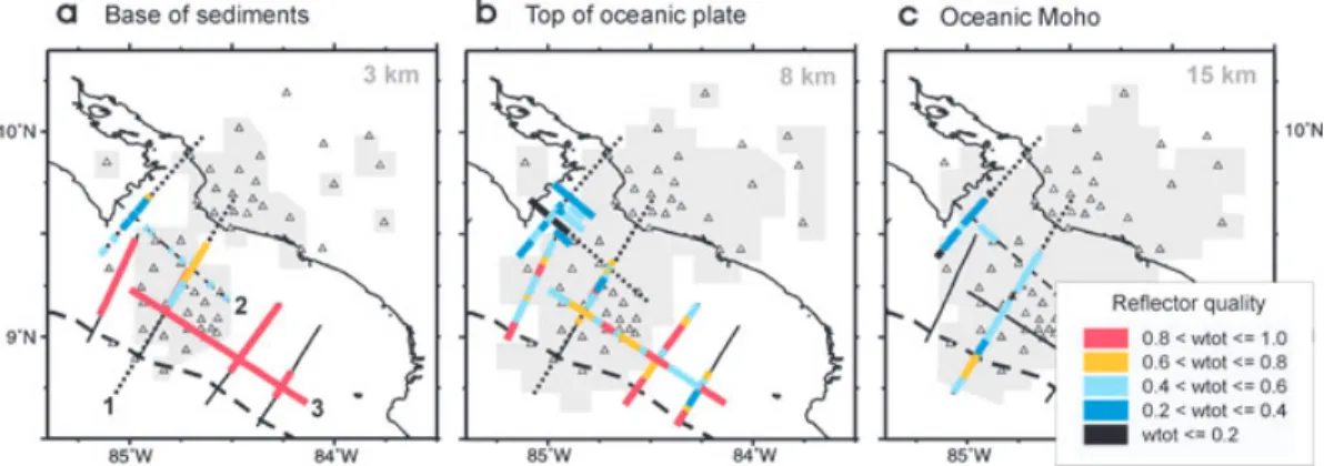
Figure 2. Controlled source seismology profiles in the study area. Dotted lines represent wide-angle profiles and continuous lines, depth-migrated near-vertical reflection profiles. Superimposed are locations of 2-D migrated reflector elements from the base of the slope sediments and the top and Moho of the oceanic plate. The inset shows the colour scale for total quality weighting factor. The grey areas indicate zones of good resolution of local earthquake tomography at 3, 8 and 15 km depth from (a) to (c), respectively. Triangles denote seismic stations of Jac´o experiment, and the position of the Middle America Trench is indicated by a dashed line. 1: profiles SO81-200 and SO81-13; 2: profile SO81-100 and 3: profile SO81-06 (see text for references).
model. For that reason, only the P-wave modelling is presented in this work.
3.2 Controlled-source seismology (CSS) profiles in the area
In a LET of Switzerland, Husen et al. (2003b) successfully used the 3-D Moho topography and associated P-wave crustal velocities modelled by Waldhauser et al. (1998) from CSS profiles from all over the country as starting model. In that way, they combined both, passive and active experiment data sets in the LET while exploiting the strength and information of each. Unfortunately, although sev-eral CSS lines traverse the area of this study, they are not distributed in a network dense enough to allow for off-line migration using the interpolation scheme from Waldhauser et al. (1998). Nevertheless, a priori information, such as velocities and thickness of sedimen-tary basins, can be used to ‘tune’ the reference model, in this case the minimum 1-D model for the data set, adjusting the modelling in zones that cannot be resolved by LET. Moreover, the interpre-tation of observed tomographic anomalies is greatly facilitated by correlation with structures well resolved by near-vertical reflection techniques.
Of particular interest for the area surveyed by the Jac´o experi-ment is the CSS profiling carried out in the Nineties by the German projects PACOMAR and TICOSECT, which aimed to explore the margin wedge and the oceanic plate structure (Hinz et al. 1996; Ye et al. 1996; Stavenhagen et al. 1998). We extracted informa-tion from four CSS profiles, whose locainforma-tion is shown in Fig. 2, to combine it with the LET: depth-migrated reflection lines SO81-06 (Ranero & von Huene 2000) and 13 (Ranero, personal communica-tion), and wide-angle profiles SO81-200 and 100 (Ye et al. 1996). Profiles SO81-13 and SO81-200 are coincident. Profile SO81-100 runs parallel to the trench across the continental slope, and traverses line SO81-200. Unfortunately, the central profile from TICOSECT possesses low quality due to high-amplitude coherent noise, which caused an apparent lack of reflections from the plate boundary zone (McIntosh et al. 2000).
Profile SO81-200, with an average shot spacing of 150m, presents relatively good coverage and reversed observations from six OBH and two land stations distributed along 125 km. It illuminated the margin structure down to 25 km depth and was analysed by Ye
used the outline of the crustal and sedimentary structure provided by near-vertical reflection data. Wide-angle line SO81-100 included five OBH recording the shooting, but only the sedimentary layer and the top of the margin wedge were well resolved (Ye et al. 1996). Deeper velocities were constrained with those from line SO81-200. Prestack depth migration has been applied to the reflection lines. The iterative migration procedure uses velocities constrained with focusing analyses and common reflection point gathers. Resolution at∼10 km is ∼0.5 km (Ranero & von Huene 2000).
Before using the information from CSS models, the reliability of the structural information needs to be assessed in terms of its un-certainty. We inspected the available CSS profiles crossing the area of this study and extracted the reflectors belonging to the slope sed-iments basement, known as ‘rough surface’ (Shipley et al. 1992), and to the top and the Moho of the subducting plate (Fig. 2). Quality factors were then assigned to the reflectors following the weight-ing scheme developed by Baumann (1994). The reflector elements from wide-angle models are weighted according to the data confi-dence (phase correlation, interpretation method), profile orientation in respect to the 3-D tectonic setting and profile type (reversed, un-reversed). Reflector elements from near-vertical reflection profiles are ranked after the quality of their reflectivity signature, migration type (i.e. source of velocity used for migration) and projection dis-tance. The total weighting factor (wtot) for each reflector is obtained by multiplying the individual factors.
Fig. 2 shows the location of the CSS profiles in the studied area, with the identified 2-D migrated reflectors superimposed and colour-coded according to their quality. For example, a reflector element from a wide-angle profile exhibits maximum quality (wtot= 1.0) when the phase picking is very reliable, the line is oriented along strike and the ray coverage is reversed. The reflector element from the oceanic Moho in wide-angle line SO81-200 that starts under the trench axis and stretches∼10 km seaward received a wtot0.64 (Fig. 2c). This value resulted from confident phase recognition (0.8), the profile orientation perpendicular to the strike (0.8) and a good reversed ray coverage (1.0).
In general, the rough-surface reflectors from reflection lines present highwtotvalues, while those from wide-angle are middle to good (Fig. 2a). Most of the reflectors from the top of the subduct-ing plate from wide-angle profiles have weightsubduct-ing factors from low to middle, the values being somewhat higher from reflection lines (Fig. 2b). The latter do not provide information from the Moho; middlewtot values are associated to the available Moho reflectors from wide-angle lines (Fig. 2c). The grey shaded areas in Fig. 2 mark the regions well resolved with our LET, according to criteria discussed later, at 3, 8 and 15 km depth, approximately the depths at which the ‘rough surface’ of the upper plate, and the top and Moho of the oceanic plate are expected, respectively. These are the areas were we can incorporate the CSS information into the LET, because they are resolved by both methods.
4 M E T H O D
4.1 Minimum 1-D velocity model
Linearization of the non-linear, coupled hypocentre-velocity prob-lem demands initial velocities and hypocentre locations to be close to their true values. Moreover, results of LET and their reliability estimates strongly depend on the initial reference model (Kissling
et al. 1994). We used the VELEST software (Kissling et al. 1995)
to determine hypocentres and the minimum 1-D P-wave velocity
model (Kissling 1988; Kissling et al. 1994) for the data set, that is, the velocity model and station corrections that most closely re-flect the a priori information obtained by other studies, but at the same time lead to a minimum average of root mean square (rms) of traveltime residuals for all earthquakes. VELEST deals with the coupled hypocentre-velocity problem by performing several simul-taneous inversions of hypocentral parameters, 1-D velocity models and station corrections.
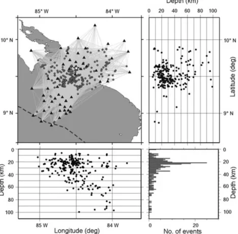
A very high-quality subset of 261 earthquakes was selected for the derivation of the minimum 1-D P-wave velocity model. These events present a maximum azimuthal gap in station coverage (GAP) of 180◦or less, show at least 12 P-wave arrival observations with the lowest reading uncertainty (±0.05 s, corresponding to weight 0) and at least one observation within a distance of 1.5 times their focal depth. Fig. 3 shows the spatial arrangement of the subset, together with the ray coverage and the hypocentre distribution in depth. A total of 4986 P-wave observations from 57 stations integrate the subset. As a result of geometrical considerations and the limits of the target area for the LET, we included readings from only 10 of the total RSN stations in the subset. The data set represents a fair sampling of the seismicity recorded over the period of the deployment: most of the events originated offshore, beneath the continental shelf, while fewer were generated within the subducting slab and the continental crust (Figs 1 and 3).
The ray tracer implemented in VELEST assumes that all the sta-tions are located within the first layer of the velocity model. For the Jac´o array, this implies a thickness of∼7 km for the first layer, because the highest land station and the deepest OBH were located at 3487 and 3561 m over and below the sea level, respectively. Near-surface velocities usually exhibit a strong gradient, therefore such an unrealistic first layer with constant velocity introduces instabil-ities in the inversion procedure, preventing convergence. Station elevations were therefore neglected during the 1-D inversions. This exclusion implies that the resulting station corrections encompass, not only the effect of the subsurface geology and large-scale ve-locity heterogeneities such a dipping slab, but also of the station elevations.
Determination of the minimum 1-D model is a trial-and-error process, in which a wide range of starting velocity models are tested in order to thoroughly explore the solution space. From ini-tial inversions with several starting velocity models with different layering (e.g. Matumoto et al. 1977; Ye et al. 1996; Quintero & Kissling 2001) we observed low velocities (<3 km s−1) in the first kilometres, and strong variation at depths from 10–15 km and un-der 40 km. A relative good convergence was found between 15 and 40 km depth. After adjusting the layering to the depth distribution of the events in the selected subset, further trials of velocity models were conducted, including high- and low-velocity tests to investi-gate the dependence of the solution on the initial model. These tests confirmed that the number and distribution of hypocentres shal-lower than 15 km and deeper than 40 km were not favourable to resolve those layers. Since most of the events recorded by the Jac´o network are located in the area where the wide-angle seismic lines SO81-100 and 200 were shot (Figs 1 and 2), the velocities for the first 15 km from the model of Ye et al. (1996) were adapted into the initial models and were overdamped during the inversion process. Table 1 shows the final 1-D velocity model.
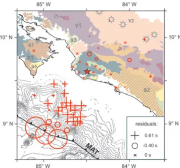
The station corrections, shown in Fig. 4, display a meaningful pattern concerning the geometry of the network, distribution of earthquakes and geological setting, as well as the effect of the station elevations. The reference station was located at 160 m a.s.l. in the Herradura Promontory. The high negative delays for the OBH at the
832 I. G. Arroyo et al.
Figure 3. Distribution of 261 hypocentres selected for determination of the P-wave minimum 1-D model, in map view and vertical cross-sections in E–W and N–S directions. Locations estimated using the 1-D model for Costa Rica from Quintero & Kissling (2001). Only events with at least 12 P-wave observations and a GAP of 180◦or less were used. At the lower right corner, a histogram of hypocentre-depth distribution is included. Black triangles represent stations. Grey lines show ray paths between epicentres and stations. Reference station is represented with a white star. The axis of the Middle America Trench is indicated by a dashed line.
Table 1. Minimum 1-D P-wave ve-locity model for Jac´o experiment. Depth (km) Vp (km s−1) 0 2.50 2.5 4.90 5 5.06 7.5 5.23 10 5.50 15 6.05± 0.05 20 6.63± 0.03 25 6.95± 0.06 30 7.23± 0.08 35 7.35± 0.11 40 7.35± 0.12 50 7.50 60 7.90 80 8.20 100 8.30
southwestern end of the network compensate for the depths close to the trench and the high velocities expected from the subducting oceanic crust. A consistent positive-correction behaviour is seen for most of the OBH located over the continental slope, where low velocities (2.1–2.9 km s−1) from the 2–3 km-thick slope sediments were modelled by Ye et al. (1996). Two OBH placed inside of a broad embayment (Fig. 4) display positive corrections lower than the rest of the stations in the continental slope. This could be attributed to the
effect of their deeper locations (∼2 km). No corrections or relatively low negative corrections (<–0.4 s) resulted for onshore stations from the Jac´o network, as expected from elevations and subsurface geology similar to those of the reference station. The positive delays for RSN stations located towards the volcanic front exhibit the influence of their altitude, somewhat weaker than expected, probably because of higher near-surface velocities.
The final average rms and variance for the data set are 0.129 s and 0.021 s2, respectively, in contrast with the initial values of 0.325 s and 0.036 s2 from the single-event mode location using the 1-D model from Quintero & Kissling (2001).
Stability tests are required for testing the robustness of the min-imum 1-D model, yielding insights into the coupled hypocentre-velocity problem for the specific data set and allowing the detection of eventual outliers as well. Following Haslinger et al. (1999) and Husen et al. (1999), we conducted several tests with randomly and systematically shifted hypocentre locations. For the first series of tests, hypocentres resulting from the inversion procedure were shifted randomly up to a maximum of 10 km in any direction, and the inversions were performed both, keeping the model fixed and with a floating model. Both cases show a very good retrieval of the original hypocentre locations, indicating that they are not system-atically biased and in the latter case, variations in velocities and station corrections are very close to the originals. The robustness of the minimum 1-D model was tested by systematically shifting all the hypocentres 10 km deeper, and inverting again both, with fixed and floating model. While recovery of the original hypocentre
Figure 4. Final P-wave station corrections for the minimum 1-D model. Reference station is marked with a star. The inset indicates the sign and scale for the station corrections. Bathymetric contours every 200 m from von Huene et al. (2000). MAT: Middle America Trench. Geology based on Denyer & Alvarado (2007): b1: tholeiitic basalts, pre-Campanian to lower Paleogene; i1: intrusives (gabbro to granite), Miocene to Pliocene; v1: vol-canism (basalt to dacite), Miocene to Pliocene; v2: volvol-canism (basaltic andesite), Pleistocene-Holocene; s1: turbiditic sequences, Campanian to Eocene; s2: turbiditic and subcoastal to coastal deposits, Oligocene to Miocene (hatched pattern: T´erraba Formation); s3: coastal and subcoastal deposits, Miocene; s4: coastal and fluvial deposits, Plio-Pleistocene. Areas in white are Quaternary continental and coastal sediments. Radiating circles denote Holocene volcanoes in central Costa Rica.
locations in the first case is excellent, they remain close to their shifted positions in the second case. These results indicate a good degree of independence of the epicentres from the velocity struc-ture, and a substantial coupling between the velocity and the depths/origin times.
4.2 Local earthquake tomography
We used a damped, least-squared iterative solution, the com-puter code SIMULPS, to solve the non-linear tomography prob-lem (Thurber 1983; Eberhart-Phillips 1990; Evans at al. 1994). Hypocentre locations are treated as unknowns in the inversion as a result of the coupling of hypocentre locations and velocities. Each iteration consists of an inversion for velocities and for hypocentre locations. After each iteration, new ray paths and traveltime residu-als are computed using the updated velocity model.
We chose the special version SIMULPS14, which has been mod-ified by Haslinger (1998) to include, besides the standard approxi-mative pseudo-bending ray tracer (ART), the full 3-D shooting ray tracer algorithm (RKP) from Virieux & Farra (1991) for the for-ward solution. It has been demonstrated that for ray paths longer than 60 km the RKP method yields significantly smaller errors than the ART (Haslinger & Kissling 2001).
Previous to 3-D modelling, the entire Jac´o database was relocated using the minimum 1-D model with station corrections derived be-fore. Since the coupling between hypocentre locations and seismic velocities demands a careful choosing of events used in the 3-D inversion, we selected a high-quality data set, including only events
with a GAP of 180◦or less and at least 8 P-wave arrivals. This data set encompasses 595 earthquakes with 11 310 P-wave observations (Fig. 5), with an average of 19 observations per event. Most of the events are located between 10 and 30 km depth, beneath the con-tinental shelf, while the rest were generated at the Wadati-Benioff zone to depths of around 100 km, at the continental crust and at the oceanic crust close to the trench.
The first inversions revealed that neglecting station elevations during the calculation of the minimum 1-D model, as described before, caused strong coupling between hypocentres and the station corrections for the data set. For this reason, and since the locations resulting from the 1-D inversion are already close to their true values, the hypocentre parameters were kept fixed during the first iteration of the 3-D inversion, while adjustments were allowed only to the velocities. Subsequent iterations permitted updating of both, hypocentre locations and velocities.
The results and the resolution estimates, such as the diagonal element of the resolution matrix (RDE), are strongly affected by the damping parameter. The damping depends mainly on model parametrization and on the average observational error (Kissling
et al. 2001). In this study we selected a value of 100, following the
approach of Eberhart-Phillips (1986). We analysed trade-off curves between model variance and data variance (Fig. 6), constructed af-ter two iaf-terations applying damping parameaf-ters ranging from 1 to 10 000. The chosen damping value ensures the largest decrease in data variance without causing a strong increase in model vari-ance, leading to the smoothest solution to fit the data. Fig. 6 also displays the trade-off curve for converged solutions, that is, when the inversion process has ended. Values lower than 100 result in a nearly constant data variance while model variance considerably increases, rendering rough models. A damping parameter of 100 also produces the data variance which more closely approaches the average weighed error of observed P-wave arrival picks and at the same time generates the minimum increase in model variance. It also indicates that noise is not being fit during modelling.
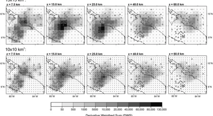
In SIMULPS14, the velocity model is defined at grid nodes re-sulting from intersecting lines in x-, y- and z-directions. Velocities are linear-interpolated between the grid nodes. Initial velocities for the LET were taken from the minimum 1-D model and interpolated at depth to match the gradient required by SIMULPS14 (Fig. 7). The grid spacing was selected to account for the distribution of stations and seismicity, aiming to obtain the highest possible uniformity in ray coverage and crossfiring without appealing to the use of uneven grid spacing, which complicates interpretation of results and reso-lution assessment (Kissling et al. 2001). Velocities were kept fixed at grid nodes that were not hit by any ray and, additionally, for those with a derivative weighted sum (DWS) value of less than 8.
We inverted first for a conservative horizontal grid of 15 km× 15 km and a vertical node spacing of 7.5–10 km for shallow depth
(<30 km) and 20 km at greater depth. Subsequent analysis of
res-olution and tests with synthetic data indicated that we could use a finer horizontal grid spacing of 10 km× 10 km without decreasing the resolution quality. The distribution of the DWS, a measure of the ray density, is as homogeneous for the 15 km× 15 km as for 10 km× 10 km grid spacing, although absolute values are smaller (Fig. 8).
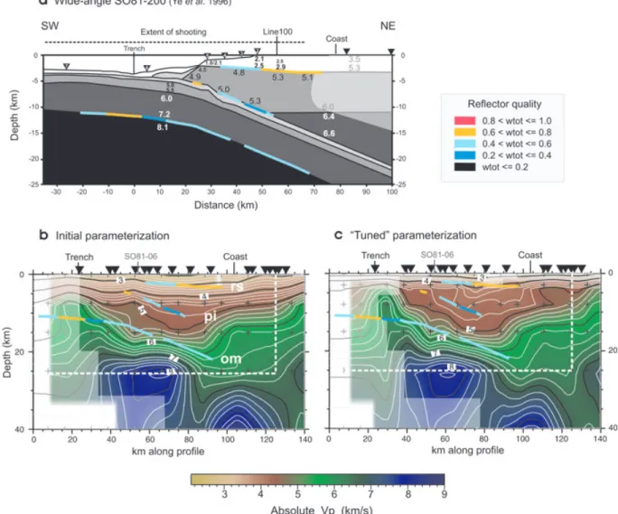
At this stage of the modelling we inspected the tomographic results in the light of the information provided by the CSS profiles. A first comparison of the absolute velocity distribution from the LET with profile SO81-200 (Fig. 9a) in areas well resolved by both methods revealed a fairly good agreement (Fig. 9b), considering the differences in type of data and techniques. Nevertheless, absolute
834 I. G. Arroyo et al.
Figure 5. Hypocentre locations of 595 events selected for tomographic inversion, shown in map view and vertical cross-sections in E–W and N–S directions. At the lower right corner, a histogram of hypocentre-depth distribution is included. Black triangles represent stations. Approximate ray coverage is shown by grey lines connecting epicentres and stations. Small circles denote final, 10 km× 10 km horizontal grid-node spacing. The axis of the Middle America Trench is indicated by a dashed line.
Figure 6. Trade-off curves of data versus model variance, constructed with results after two iterations (triangles) and from the converged solution (cir-cles). Tested values of damping parameter range from 1 to 10 000 as indi-cated. For reasons of space and clarity, extreme values of the test are omitted. The square marks the chosen damping parameter. The dashed line represents the average weighed error of observed P-wave arrival picks.
velocities obtained with the LET are lower and the velocity contrasts are located deeper than in the CSS model.
Seeking to include as much information as available for the area in the 3-D inversion, and given that near-surface velocities are more reliably estimated by CSS data, we modified the original upper ver-tical grid spacing in order to mimic the∼3-km-thick sedimentary coverage of the margin wedge with its corresponding velocity gradi-ent, as shown in Fig. 7. The 3-D inversion resulted in a better match between the tomographic image and the velocity gradient given by
Figure 7. Velocity gradient and vertical grid nodes distribution for the 3-D inversion. The dashed line represents the original parametrization; the continuous line, the final starting model after ‘tuning’ with information from controlled source seismology.
Figure 8. Derivative weighted sum (DWS) distribution in some horizontal depth sections for two different model parametrizations, as indicated. Triangles represent stations and small crosses denote grid nodes. The axis of the Middle America Trench is indicated by a dashed line.
the CSS model (Fig. 9c). Absolute velocities display a good con-cordance between both models in the upper oceanic crust (5.0– 5.3 km s−1), the continental crust (3.5–6.5 km s−1) and specially in the margin wedge (3–5 km s−1). Tomographic velocities in the lower oceanic crust and in the oceanic mantle, though, are very similar in both coarse and finer, ‘tuned’ tomographic images and remain lower than the values from wide-angle modelling at the same depths. The latter, however, are determined from unreversed observations and are thus coupled to the uncertainty in the depth of the Moho.
The subducted seamount associated with the Jac´o Scar, located ∼20 km inward from the trench axis (Fig. 1), is another feature, which provides linking between the tomographic results and the CSS models. The seamount was clearly depicted as a low-velocity anomaly in the tomogram of the inversion using the coarse horizon-tal grid (Fig. 10a). This seamount has been displayed by reflection lines SO81-06 and 13 (von Huene et al. 2000), which cross each other, and by gravimetric modelling (Barckhausen et al. 1998), in an area where its presence was previously suspected from images of high-resolution bathymetry: a portion of the margin slope is dis-rupted, showing a doming in the middle continental slope and a scar left by the failure of the slope sediments (von Huene et al. 1995, 2000). Nevertheless, reducing the horizontal grid spacing to 10 km× 10 km and introducing a closer vertical spacing in the upper 10 km had a negative effect on the definition of the seamount image, as shown in Fig. 10(b). This loss indicates a decrease in the resolution capability in this area due to limited ray coverage. Moreover, introducing grid nodes at 3 km depth with higher veloc-ities than in the original inversion modifies ray paths and reduces the velocity gradient between 5 and 10 km depth, resulting in a weaker contrast of the low-velocity anomaly at those depths. In a good example of the significance of parametrization in tomography, particularly when studying velocity structure details, we were able to improve the seamount image in the finer grid by slightly shifting (∼6 km to the southwest) the location of the fine grid nodes so that
a grid node coincides with the seamount position as estimated by CSS lines and the coarse LET (Fig. 10c).
The final tomographic model achieved a data variance reduction of 66 per cent compared to the 1-D reference model. The final weighted rms over all traveltime residuals is 0.083 s. This value is close to the a priori observational error, indicating convergence of the inversion.
4.3 Solution quality
The heterogeneous arrangement of sources and receivers in a LET limits the area of good resolution and may lead to the introduction of artefacts. In general, the solution quality of a certain volume depends mainly on the geometrical distribution and density of rays. Classical tools to asses ray coverage include the display of resolu-tion estimates such as hit count, derivative weighted sum (Fig. 8), diagonal elements of the resolution matrix (RDE), and the spread function (see e.g. Reyners et al. 1999; Husen et al. 2000). Tests with synthetic data are a powerful tool, not only to gain useful in-formation about model parametrization and damping, but to define areas of good and low resolution (Kissling et al. 2001). These tests consist of the construction of synthetic input velocity models and the computation of synthetic traveltimes using the same source– receiver distribution of the real data set, and of inversion applying identical model parametrization, damping, and number of iterations as for the real data.
We undertook at first two types of synthetic tests, checkerboard and characteristic models (Haslinger & Kissling 2001) and, consid-ering the results of the inversion of real data, we further designed a synthetic model to test for slab structure. The synthetic travel-times through the models were calculated using the finite-difference technique of Podvin & Lecomte (1991). Gaussian-distributed noise proportional to the original observational uncertainty was added to the traveltimes.
836 I. G. Arroyo et al.
Figure 9. Comparison between wide-angle profile SO81-200 model (Ye et al. 1996) and local earthquake tomography results. Cross-sections (b) and (c) display absolute velocity tomograms coincident with profile SO81-200, using initial and ‘tuned’ parametrization (see text for description), respectively and including reflectors from the sediment cover (rs), the top of the slab (pi) and the oceanic Moho (om) from that profile, as indicated. Areas of lesser resolution are masked. Colour code for reflector quality as in Fig. 2. Profile location is given in Fig. 2. Dashed line in (b) and (c) marks the area modelled by profile SO81-200. Inverted triangles represent stations.
We performed synthetic checkerboard tests in order to explore the regions of the model where it is possible to resolve small-scale structures (see Fig. S1). Following Husen et al. (2004), two checkerboard models were designed, each consisting of alternating high- and low-velocity anomalies (±10 per cent) with one grid node left open in between to test for horizontal smearing; at the same time, every other layer is free of anomalies to test for vertical smearing. One model has anomalies placed at 0, 8, 25 and 60 km depth, and the other at 3, 15, 40 and 80 km depth. The tests were conducted for anomalies spanning over two grid nodes in x- and
y-direction (Fig. S1a), and repeated for anomalies encompassing
just one grid node (Fig. S1b). As an example, Fig. 11 presents only the results from the checkerboard tests using the second model and one-grid node anomalies. The resolution is very good both off and onshore, even at depths greater than 40 km and with one-grid anomalies. As expected from the earthquake distribution (Fig. 5), at 60 km depth resolution is still good onshore, also for the model with one-grid anomalies. Vertical smearing is low at all depths, but it is slightly stronger in the first 8 km. Starting at 25 km depth, some minor horizontal smearing oriented northeast–southwest is
detected offshore. Amplitude recovery is also good, reducing to a more moderate ability between 40 and 60 km depth.
Since checkerboard tests cannot ensure that the data set is able to resolve larger scale structures (Leveque et al. 1993), following Haslinger et al. (1999) and Husen et al. (2000) we designed an input characteristic model, based on the inversion results obtained with the real data set (see Fig. S2). This synthetic model retains the sizes and amplitudes of anomalies seen in the tomographic im-ages but with rotated shapes and different signs. Areas of good resolution are those, which show a good recovery of the synthetic model. In agreement with the checkerboard tests, we observe that the central part of the modelled area is well resolved down to depths of 60 km, with resolution decreasing with depth. Horizontally, the well-resolved area extends from the trench, until 25 km depth, to the volcanic front. The area resolved at 40 and 60 km depth is broader to the southeast because the deeper earthquakes used for the tomography occur closer to the trench there. A very good re-covery of boundaries between high- and low-velocity anomalies is observed. Amplitude restitution is excellent from 3 to 25 km depth, although at levels shallower than 10 km the recovery is patchy. At
Figure 10. Effects of different model parametrizations on the tomographic image of Jac´o seamount. Cross-section (as indicated) and depth slice from: (a) coarse horizontal grid of 15 km× 15 km; (b) horizontal grid 10 km × 10 km, tuned vertical grid; (c) horizontal grid 10 km × 10 km, tuned vertical grid and slight shifting of the coordinates origin of the horizontal grid. Grey lines encompass well-resolved areas as indicated by different resolution tests (see text for details). Triangles represent stations, and the dashed line the Middle America Trench. See text for discussion.
Figure 11. Horizontal depth sections with assessment of solution quality using synthetic checkerboard models. Recovered model is shown in plane views at different depths, as an example of the checker models with one-grid sized anomalies (see text for explanation). Locations of high (+10 per cent) and low (–10 per cent) velocity input anomalies are shown by blue and red squares, respectively. Small crosses represent grid nodes of the model parametrization, grey triangles denote seismic stations. The axis of the Middle America Trench is indicated by a dashed line.
838 I. G. Arroyo et al.
40 km depth the amplitudes are more reduced, ranging from∼60 to 80 per cent, and at 60 km and deeper, recovery is ∼60 per cent. Some horizontal smearing is observed offshore again at 40 km depth, probably caused by the fact that earthquake hypocentres deeper than 30 km are found towards the volcanic front, generating ray paths to the OBH oriented mostly northeast–southwest.
We examined also values and pattern of the RDE and the resolu-tion contours (see Fig. S2), which help to visualize the orientaresolu-tion and spatial bias of possible velocity smearing in 2-D, that is, the de-pendency of the solution of one model parameter on its neighbours (Reyners et al. 1999). An excellent correspondence is observed between areas considered as well resolved according to the char-acteristic model test and the RDE values, and the areas outlined by resolution contours where the off-diagonal elements of the res-olution matrix are still 70 per cent of the corresponding diagonal element. The RDE values of the model range from 0.01 to 0.73; most are between 0.05 and 0.40. These values are the result of the model parametrization and the damping, both conservatively
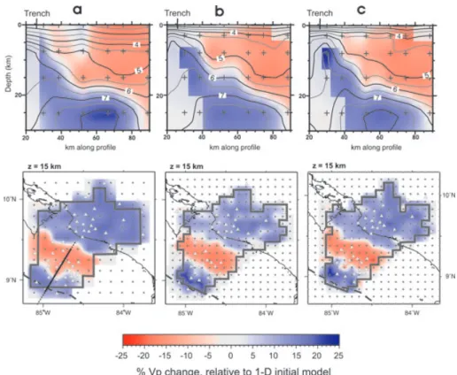
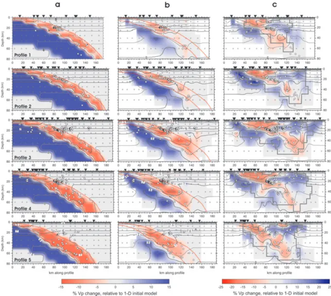
cho-Figure 12. Synthetic test to examine the ability of the data to solve the observed slab structure. Column (a) shows the model used to derive synthetic traveltimes, while column (b) displays the results of their inversion. For comparison, column (c) presents the tomograms using the real data. Cross-sections show velocity structure as percentage change relative to the minimum 1-D model derived in this study; contours correspond with absolute velocities. Location of the cross-sections is given in Fig. 1. Earthquakes located within 8 km of either side are projected onto the profiles (white circles). Inverted triangles represent stations and small crosses denote grid nodes. Dotted red lines delineating the band of low velocities are added to ease comparison.
sen. Additionally, comparison with areas qualified as well resolved by the characteristic-model test yields a cut RDE value of 0.04 for good resolution. As indicated by the resolution contours, signifi-cant smearing for depths greater than 3 km occurs only at model parameters located at the edges of the volume.
As seen partially in Fig. 10 and described later in the results section, from the trench down to 60–70 km depth the tomographic images illuminate the general configuration of the margin as a high-velocity subducting slab with a band of low velocities on top. In order to test the ability of the data to resolve this structure, we calculated synthetic traveltimes through a model consisting of a high-velocity slab (+15 per cent) overlain by a relatively thin band of low velocities (–10 per cent), displayed in Fig. 12(a). Between 15 and 65 km depth, the vertical grid spacing of this synthetic model is 10 km, which is closer than the parametrization of the real model, making it more realistic. A thickening of the LVB towards the east mimics the results obtained using the real data. Modelling using the same inversion parameters determined for the real data set gave the
results presented in Fig. 12(b). Column (c) in Fig. 12, showing the results with real data along the same profiles, has been added to ease comparison and discussion.
Fig. 12(b) shows that, although decreased towards the borders, the amplitude recovery of the model is very good along the studied portion of the margin. In the centre of the model (profiles 2–4), the high velocities of the slab are well recovered from the trench down to 40 km depth. Amplitudes are slightly decreased below that depth but the continuity of the slab is still clearly displayed. At the edges of the model volume (profiles 1 and 5), amplitudes are significantly reduced, but the slab still appears as a continuous feature. Comparison of amplitude restitution from profiles 1 to 5 indicates a lateral change in resolution from northwest to southeast, with mainly the upper or the lower part of the volume well resolved, respectively. The band of low velocities on top of the subducting slab is well recovered between 15 and 25 km depth along all profiles. At 40 km depth low velocities are well recovered along profiles 3– 5, where it appears as a continuous band. Between kilometres 130 and 150 along profile 3 there is a leakage of low velocities from the slab into the overlying forearc mantle, caused by rays travelling through the slab and upward towards the stations located onshore. In summary, the tests revealed that we can reliably image a low-velocity zone and its eastward thickening on top of a high-low-velocity slab throughout our model. An additional test using a synthetic model with a thin, uniform LVB showed equally good recovery, increasing our confidence in the capability of the data to reproduce a real feature (see Fig. S3).
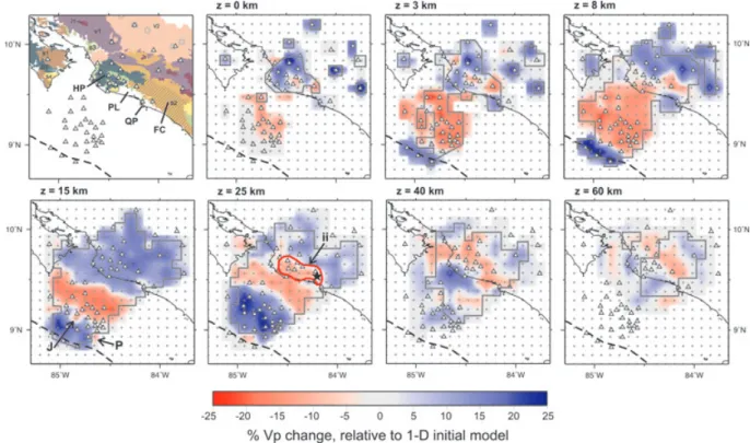
Figure 13. Tomographic results of 3-D P-wave velocity model shown at different depths. Velocity perturbations relative to the minimum 1-D model are shown with red to blue colours, for velocities lower and higher than predicted by the minimum 1-D model derived in this study, respectively. Areas with no ray coverage are masked. Dark grey lines contour areas of RDE> 0.04 (see text for discussion). At 25 km depth, red lines contour the low-velocity anomaly ii, observed below the inner forearc (see text for discussion) and the star, the epicentre of the 2004 Mw6.4 earthquake (Pacheco et al. 2006). Triangles
represent stations and small crosses denote grid nodes. The axis of the Middle America Trench is indicated by a dashed line. HP: Herradura Promontory, QP: Quepos Promontory, PL: Parrita lowland, FC: Fila Coste˜na (hatched pattern), J: Jac´o seamount and P: Parrita seamount. Geology as indicated in Fig. 4.
5 R E S U L T S
The tomographic results are presented in several depth slices (Fig. 13) and vertical depth sections perpendicular to the trench (Fig. 14), whose locations are shown in Fig. 1. Depth sections show Vp in relative and absolute values. The indicated areas of good resolution have been defined following the previous discus-sion on the solution quality. In general, the tomographic model has a good resolution from the trench to the southwestern flank of the volcanic front, varying in the vertical direction down to depths of 60–70 km in the northwest and central parts of the area, and of 80 km in the southeast. We describe the results by regions, refer-ring to the east, central and west zones of the studied area, which along the coast correspond to the entrance of the Nicoya Gulf, the Herradura Promontory and the Parrita lowland, respectively (Figs 1 and 13).
In an attempt to define the top of the subducting plate, as shown in Fig. 14, we consider the position and depth of the trench axis (3.3–3.7 km), absolute velocity values and velocity perturbations, as well as the distribution of the intraslab and interplate seismicity, which forms a clear dipping planar feature (Figs 12 and 14). The model of Ye et al. (1996) for profile SO81-200 predicts velocities in the upper oceanic crust between 5.0 and 5.5 km s−1 (Fig. 9a). Applying those values as a guide in our model renders coherent results with the interplate seismicity for the first 15 km. At greater depths we use the clear contrasts between high- and low-velocity anomalies, and the distribution of the intraslab seismicity.
840 I. G. Arroyo et al.
Figure 14. Vertical depth sections along the Central Pacific margin off Costa Rica showing the 3-D P-wave velocity structure. Location of profiles are indicated with dashed lines in Fig. 1. Column (a) shows velocity structure as percentage change relative to the minimum 1-D model; grey lines contour areas of RDE> 0.04 (see text for discussion). Column (b) presents absolute velocities; areas of good resolution are shown in full colours, areas of lesser resolution in faded tones. Earthquakes located within 8 km of either side are projected onto the profiles (open circles). Inverted triangles represent stations and small crosses denote grid nodes. Bold lines indicate the position of the plate interface and the continental Moho (dotted) as interpreted in this study (see text). The bottom of the low-velocity band (LVB) on top of the slab (see text for explanation) is delineated by red (column a) and white (column b) lines, dashed over artefacts interpreted from test for slab structure (Fig. 12). Anomalies i and ii as indicated in the text. Stars represent 1990 Mw7.0 (profile 1) and 2004 Mw6.4 (profile
5) earthquakes, from Husen et al. (2002) and Pacheco et al. (2006), respectively. T and C represent the trench and coast locations, respectively. HP: Herradura Promontory, FC: Fila Coste˜na (Coastal Range), Ms: Miocene coastal deposits, MPv: Miocene–Pliocene magmatic front, Pv: Pleistocene volcanism, PHv: Holocene volcanic front, Co: C´obano seamount and J: Jac´o seamount.
5.1 Near-surface geology
Although the resolution at sea level is restricted to relative small areas and some velocity smearing has been detected, several clear anomalies there and at 3 km depth reflect very well the near-surface geology (Figs 4 and 13). The oceanic-assemblage formations crop-ping out along the coast appear as high-velocity anomalies at Nicoya Peninsula and the Herradura and Quepos promontories, with ab-solute values between 3.0 and 5.4 km s−1. The Pleistocene debris-flows (alluvial) deposits that outcrop northwestward from Herradura and the underlying Miocene coastal sedimentary rocks (Fig. 4) are congruously imaged as a low-velocity anomaly. The Pleistocene volcanic front and the volcanic formations from a previous, Miocene–Pliocene magmatic front located closer to the coast rep-resent high-velocity perturbations. The extensive negative anomaly expanding from the trench towards the coast with velocities from 3.8–4.6 km s−1could be related to both, the upper part of the mar-gin wedge and the up to 3-km thick sediment coverage revealed by reflection profile SO81-13 (von Huene et al. 2000). The subducting plate appears at 3 km depth at the trench as a high-velocity anomaly, with maximum absolute velocities of 5.6 km s−1.
From the surface down to 8 km depth a low-velocity anomaly with absolute velocities of 4–5 km s−1 has been imaged beneath the Parrita lowland, between Herradura and Quepos (Fig. 13 and Fig. 14, profile 5) but possibly extending further to the southeast, outside of the model. The projection of the anomaly onto the sur-face coincides very well with the northeasternmost outcrops of the dense sequences of Oligocene turbidites from the T´erraba Forma-tion (Figs 4 and 13) which constitute the main part of the Fila Coste˜na (Coastal Range), an inverted forearc basin thought to have been exhumed as a response to the subduction of the Cocos Ridge (Corrigan et al. 1990). To the northwest and north, the perturbation ends sharply against a high-velocity body, possibly related to the Miocene volcanic front. The northwest end follows the strike of the Parrita fault (Marshall et al. 2000; Denyer & Alvarado 2007), which limits the Herradura Block (Fig. 4). This fault is part of an active system oriented at high angles to the margin. This system separates forearc blocks with different uplift rates, interpreted as a response to subduction of seafloor roughness (Fisher et al. 1998; Marshall
et al. 2000). Seaward, the low-velocity perturbation is limited by the
positive anomaly under Quepos Promontory (Fig. 13). Stavenhagen
et al. (1998) report that the T´erraba Basin consists of
interme-diate velocity sediments (3.0 km s−1) and to have a thickness of 2 km; Rivier (1985) estimates 3.5 km thickness on the basis of gravimetric models. The low-velocity zone of our model extends down to 8 km depth, where a down bending of the 5 km s−1 con-tour is found, but some amount of vertical smearing could slightly enlarge the image.
5.2 Subducting slab
The portion of the slab resolved by this study shows dipping angles of 10◦–12◦from the trench down to 15 km depth. The dip increases to 16◦–25◦at the seismogenic zone, from 15 to 25 km depth, and steepens further towards the east (Fig. 14, profiles 4 and 5). Deeper than 40 km the slab dips at 40◦–45◦.
The west and central zones of the margin display basically a sim-ilar velocity structure (Fig. 14, profiles 1–3), although we observe some medium-scale variations. From the Nicoya Gulf entrance to the eastern flank of the Herradura Promontory, and from the trench downward to depths greater than 60 km, the Cocos Plate is imaged as a high-velocity body with a LVB on top. The intraslab seismicity
deeper than∼30 km takes place in this band. The LVB has been delineated in the profiles in Fig. 14. Down to 20 km depth, velocity changes up to –12 per cent in the upper part of the slab; at greater profundity, maximal observed changes are of –5 per cent. The latter value could actually reach –8 per cent, taking into account that the model capacity to recover amplitudes diminishes at levels deeper than 40 km, as indicated by the synthetic tests (e.g. Figs 11 and 12). The absolute velocity along the top of the slab is 5 km s−1 down to 15 km depth; from 15 to∼25 km depth the velocity gradient increases to reach 7 km s−1, a value that persists almost constant down to 40–45 km depth. Velocities of 7.4 km s−1appear along the top of the slab at∼40 km depth in the west but at 50–55 km depth towards the centre.
The LVB is interrupted by high velocities at around 35–40 km depth, between kilometres 90–110 along cross-sections 2–5 (Fig. 14). The results of the test for slab structure (Fig. 12) dis-cussed above indicate that this gap in the LVB is an artefact only in profile 2. From the trench down to 25 km depth, the LVB encom-passes the first 5–7 km of the slab. At 25 km depth and 50–60 km from the trench, the tomographic images show a down bending of the 0 per cent Vp-anomaly contour, indicating an increase in the thickness of the LVB. In cross-sections 1–2 (Fig. 14) the thickness of the LVB increases to 10–12 km. Starting at profile 3, a pronounced down bending of the lower part of the LVB, marked as anomaly i in Fig. 14, is found along 30–40 km and between 25 and 40 km depth, specially conspicuous in cross-section 4. Absolute veloci-ties in this anomaly range from 6 to 7.2 km s−1. The LVB widens strongly downdip of this sharp contortion, encompassing more than 15 km. Neither the resolution contour maps nor the results from the test for slab structure (Fig. 12) show vertical velocity leakage or artefacts along this portion of the cross-sections. Furthermore, in-versions of the real data set using a closer vertical grid-node spacing (10 km) from 25 to 45 km depth yielded identical results, ruling out the possibility of the widening being caused by a change in the grid-node spacing.
Thus, in the east zone, coinciding with the upraise of the Fila Coste˜na onshore (Fig. 13), the margin structure changes consider-ably over a distance of only∼15 km (Fig. 14, profile 5). Besides the presence of anomaly i, the top of the slab presents here a more uniform absolute velocity gradient in the first 30 km in depth, and the LVB is notably wider at depths larger than that, comprising up to 20 km. The existence of a wider LVB in this area is confirmed by the results from the test for slab structure, which demonstrates that a high-velocity slab could be resolved (Fig. 12), even if the amplitude recovery is not optimal. Velocities of 5 km s−1 along the top of the slab are found down to 10–15 km depth; the 7 km s−1contour appears between 30 and 35 km depth. Velocities of 7.4 km s−1 at 45 km and of 7.8 km s−1at 65 km depth are probably overestimated, since amplitude recovery of the model decreases for depths greater than 40 km and in general towards the east (Fig. 12).
The reflection line SO81-06 reveals that the Jac´o seamount has ∼25 km diameter and its summit, according to the depth migration, is located at 5 km depth (Fig. 9). The tomographic image of the seamount (Fig. 10 and Fig. 14, profile 3) coincides in horizontal extend with the reflection data, appearing as a low-velocity anomaly down to 15 km depth and suggesting thickening of the oceanic crust. We observe an up bending of the contours slower than 5 km s−1, although the upper part of the seamount is difficult to define because of the similar velocities found in the overlying margin wedge. Some minor vertical velocity smearing is indicated at 8 km depth by resolution contours. Velocities higher than 5 km s−1show a down bending even at 20 km depth (Fig. 14, profile 3). To the southeast
842 I. G. Arroyo et al.
of Jac´o seamount, another seamount of similar size, closer to the trench and related to the Parrita scar on the continental slope, has been imaged outside of the area of fair resolution (Fig. 13, 15 km depth).
5.3 Margin wedge and continental crust
The east and central zones show a pronounced low-velocity anomaly in the upper plate that starts some kilometres from the trench axis and extends from the surface down to the plate interface, to a depth of∼20 km (Fig. 14, profiles 1–4). Its lower limit shallows towards the coast and finishes at∼75 and ∼85 km from the trench axis in the west and central parts, respectively. The velocity changes up to –10 per cent, with some spots reaching –15 per cent (Fig. 14, pro-files 2–3). The absolute velocities in this anomaly vary from 3.5 to 6.0 km s−1. We identify this low-velocity zone as the margin wedge, with base on results from wide-angle profiles, which present a sim-ilar velocity distribution. Low velocities are justified by the normal faulting in the margin wedge across the middle slope revealed by high-resolution seismic records (Hinz et al. 1996; Ranero & von Huene 2000). Moreover, local fluid venting form the plate interface takes place through these faults (Hensen et al. 2004). Although the uppermost 10 km do not present the best resolution between the continental slope and the coast in the east zone, the area of the margin wedge seems to narrow again, extending up to 65 km from the trench axis (Fig. 14, profile 5).
Landward, the margin wedge is laterally limited by a positive anomaly representing the continental crust. It extends down to 30– 35 km depth, where absolute velocities range from 3.0 to 7.0– 7.2 km s−1. The velocity gradient decreases at depths greater than 10–15 km, a change roughly marked by the 6 km s−1contour. The most conspicuous high-velocity anomalies, with more than 15 per cent velocity change, are located in the upper crust beneath the southwestward edge of the Miocene volcanic arc (Fig. 14, profiles 3–5).
The high velocities of the upper plate are interrupted beneath the inner forearc by a low-velocity anomaly, termed anomaly ii in Figs 13 and 14. The anomaly coincides spatially with the appearance of anomaly i and the thickened LVB on top of the slab (Fig. 14). Anomaly ii roughly emerges at the downdip end of the interplate seismicity and seems to be itself aseismic. It extends from 25 km down to 35–40 km depth, where it joins the slab top, following the coastline from beneath the west part of the Herradura Promontory until Quepos, and stretching ∼20 km landward. Absolute veloci-ties within the anomaly are 6.5–6.8 km s−1. Underneath the Parrita lowland, anomaly ii increases in amplitude and shows a more con-spicuous shape in cross-section (Fig. 14, profile 5). Eastward from Quepos Promontory the perturbation seems to disappear, although we reach there the limits of the volume illuminated by our data set (Fig. 13, 25 km depth). In their LET for Costa Rica, Husen et al. (2003a) also imaged this low-velocity anomaly and proposed that it could be caused by the presence of a subducted seamount.
5.4 Continental Moho and forearc mantle wedge
Previous works in Costa Rica determined depths between 30 and 43 km for the Moho discontinuity, and reported that the velocity con-trast between the mantle and the crust is weak (Matumoto et al. 1977; Quintero & Kulh´anek 1998; Quintero & Kissling 2001; Sallar`es et al. 2001; DeShon & Schwartz 2004). Wide-angle pro-files in the Central Pacific area (Ye et al. 1996; Stavenhagen et al.
1998) did not illuminate depths greater than∼20 km. DeShon et al. (2006) inferred the continental Moho location under Nicoya Penin-sula following a turnover of the contour for P-wave velocities of 7.0–7.2 km s−1, which they found to be in good correspondence with lower crust velocities from the refraction model of Sallar`es
et al. (2001). Our tomographic results show an increased velocity
gradient together with a clear bending of the 7.0–7.2 km s−1 con-tours, supporting DeShon et al. (2006) assumption. We observe a sharper velocity gradient in the western and central parts of the area (Fig. 14, profiles 1–3), becoming more diffuse towards the east (Fig. 14, profiles 4–5). Beneath the coast and landward, the Moho appears at 30–35 km depth (Fig. 14, profile 5). The forearc mantle wedge exhibits velocities of 7.2–7.6 km s−1in the east and the west. In the central part, slower velocities of 6.8–7.2 km s−1are modelled (Fig. 14, profile 3), but they are most likely caused by upward veloc-ity leakage from the LVZ, as indicated by the test for slab structure (Fig. 12).
6 D I S C U S S I O N
In this study, we collected information from CSS lines available in the area resolvable with LET and incorporate it indirectly into the inversion process. Usually, when CSS data are inverted directly in a LET, shots are treated as earthquakes with known origin time and location, and therefore they are not relocated during the inversion process. However, the location of the sources at the surface can negatively affect the inversion because of the stronger non-linearity resulting from the dependence of the ray turning points on the velocity structure (Laigle & Hirn 1999). Shots recorded along a seismic refraction line densely sample the wavefield in a specific direction and represent a powerful tool to obtain a model of the underlying structure, with velocities averaged along the ray paths. The data quality is often very different for CSS and earthquake data sets. Due to a better phase correlation, refraction data can often be picked with higher accuracy than LET data. Kissling et al. (1995) point out that data from experiments so different should not be mixed and treated in a similar way by a trial-and-error process that involves many inversions; rather, the data should both be used in different ways that exploit their strengths.
A good agreement is observed between the distribution of ab-solute velocities of the ‘tuned’ tomography and the 2-D model of Ye et al. (1996) for wide-angle profile SO81-200, although the ve-locity contrasts appear 2–5 km deeper in the tomograms (Fig. 9). This could be attributed to the differences in the estimation of veloc-ities of each method, as well as their inherent uncertainties. While LET yields a volume-wise average of velocity, wide-angle 2-D ray tracing modelling averages velocities along the ray path. The earth-quake distribution in 3-D ensures precise information of seismic velocities per volume, provided that there are enough rays per vol-ume, coming from different directions. Also, the location of both, sources and receivers outside the studied area restricts the ability of CSS methods to resolve the precise position and true dip of re-flecting structural elements. The strength of the wide-angle method lies in its sensibility to large-scale vertical and horizontal velocity gradients and discontinuities. Ray crossfiring is limited in 2-D CSS profiles, and the velocities resulting from ray tracing and in-line mi-gration are averages for the specific layers. On the other hand, LET resolution capability is limited by the grid-node spacing, therefore decreasing with depth.
Ye et al. (1996) do not discuss the uncertainties of their model for the wide-angle line SO81-200, but they do mention that the