Linear Stochastic Reserving Methods

BY

RENÉ DAHMS

ABSTRACT

In this article we want to motivate and analyse a wide family of reserving models, called linear stochastic reserving methods (LSRMs). The main idea behind them is the assumption that the (conditionally) expected changes of claim properties during a development period are proportional to exposures which depend linearly on the past. This means the discussion about the choice of reserving methods can be based on heuristic reasons about exposures driving the claims development, which in our opinion is much better than a pure philosophic approach. Moreover, the assumptions of LSRMs do not include the independence of accident periods.

We will see that many common reserving methods, like the Chain-Ladder-Method, the Bornhuetter-Ferguson-Method and the Complementary-Loss-Ratio-Method, can be interpreted in this way. But using the LSRM framework you can do more. For instance you can couple different triangles via exposures. This leads to reserving methods which look at a whole bundle of triangles at once and use the information of all triangles in order to estimate the future development of each of them.

We will present unbiased estimators for the expected ultimate and estimators for the mean squared error of prediction, which may become an integral part of IFRS 4. Moreover, we will look at the one period solvency reserving risk, which already is an important part of Solvency II, and present a corresponding estimator. Finally we will present two examples that illustrate some features of LSRMs.

KEYWORDS

Stochastic Reserving, Mean Squared Error of Prediction, Solvency Reserving Risk, Claims Development Result.

1. INTRODUCTION

A main task of actuaries is to analyse random claim properties and project their development. This often includes the combination of several sources of information, but most of the standard reserving models cannot properly com-bine such information. For instance, they only project payments or reported

amounts separately, but cannot combine both. In recent years several authors have studied models that can be used in specifi c situations in order to analyse different claim properties simultaneously, see for instance Quarg-Mack [12], Halliwell [5], Dahms [3] and Wüthrich-Merz [11].

In this paper we will introduce a wide class of stochastic reserving methods that can deal with several claim properties simultaneously. The main idea behind them is the assumption that the (conditionally) expected changes of claim properties during a development period are proportional to exposures which depend linearly on the past of claim properties. Therefore, we will call such methods linear stochastic reserving methods or LSRMs. Another important property of LSRMs is that they allow for various dependencies of accident periods. Many of the classical reserving methods, like the Chain-Ladder-Method, the Complementary-Loss-Ratio-Method and the Bornhuetter-Fergu-son-Method, are LSRMs, see Sections 2.1-2.4.

We will derive estimators for the ultimate outcome of claim properties (Section 3), analyse the overall uncertainty of these estimators (Section 4) and the one period uncertainty of the claims development result (Section 5). The analysis of the overall uncertainty may become an integral part of IFRS 4 and the analysis of the uncertainty of the claims development result already is an important part of Solvency II. Moreover, we will see that in the case of some classical reserving methods those estimators are the same as introduced before by other authors, see for instance Mack [6], Buchwalder et al. [2] and Dahms-Merz-Wüthrich [4].

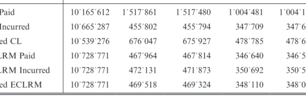
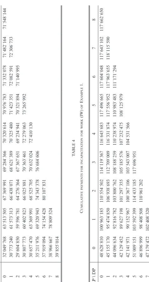
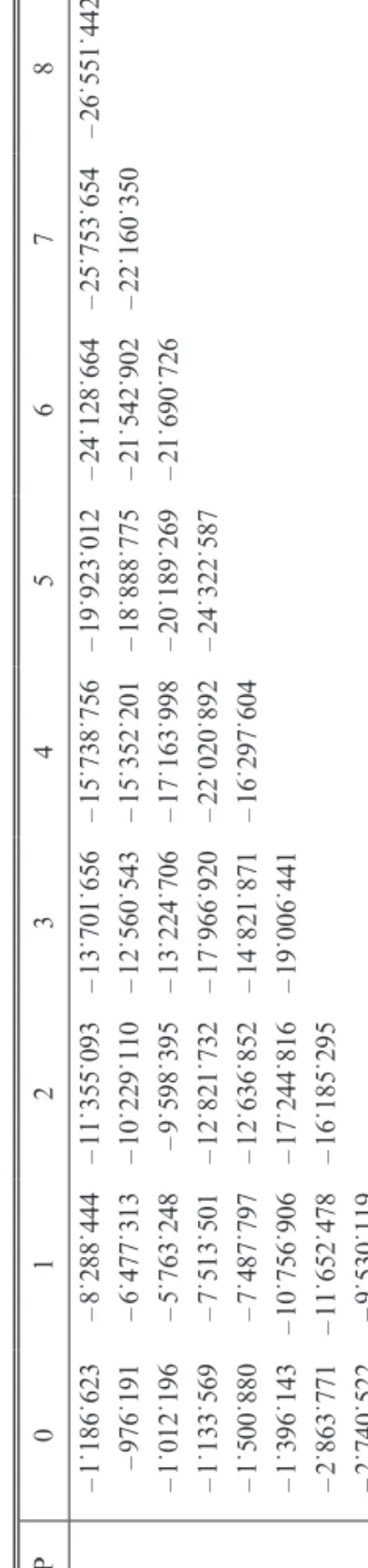
In Section 6 we will present and discuss two examples of LSRMs based on real data. We will not discus the question which method is the best for the projection of specifi c data. Although this is a very important question it is too complex for this paper. Moreover, we think that for the model selection non triangle based information is of great importance, see the example of Section 6.1, and it is very diffi cult to include such information into an analytic triangle based rating of methods.

2. THEMODEL

Let Si km, , 0 # m # M, 0 # i # I, 0 # k # J, denote the incremental value of the

m-th claim property of the i-th accident period during the k-th development period. We assume that I $ J and that there is no development of any claim property after development period J, which means we do not discuss any tail development. Such claim properties may be the usual candidates like pay-ments, reported amounts and number of reported claims or even more special constructions like payments after reopening.

Our model contains three natural time lines: accident periods or rows, development periods or columns and business periods or lower-left to upper-right diagonals. We will use the indices i and h for accident periods, j and k for development periods, l and m for claim properties and n for business periods, see Figure 1.

By Ln and Lk we denote the linear spaces generated by all increments Sim,j

up to business period n and development period k, respectively. Moreover, by Lnk we denote the linear space generated by L

n and Lk, i.e. n _: x x x i = n , , , , , , , , , i j i j i j k i j i j i j k i j i j i j L L L : : : : : S x S x S x ( (( ) j n i J i I m M j k i I m M j J i I m M 0 0 0 0 0 0 0 0 0 R R R ! ! ! = = / / = -= = = = = = -= = ) , , , m m m m m m n ) k0 m m m * * * 4 4 4

/

/

/

/

/

/

/

/

/

(2.1)

where a / b and a 0 b denote the minimum and maximum of the real numbers a and b, respectively. The s-algebra of all information of accident period i up to development period k is denoted by Bi, k. Moreover, we denote the

s-alge-bras generated by Ln, Lk and L n k by Dn, Dk and Dk n , respectively, i.e. , i j L Bi k, : S : 0 m M, 0 j k , Dk : k Bi, i I 0 # # # # = = = = s s s k , m ^ h ^ h f

'

p D : n Bi n,( i) J D : Lkn B,(( ) ) i I k i n i J k i I 0 0 = = - / = = / 0 = -= s L s s s n n , , ^ h _f

'

p ^ h f

'

p

see Figure 1. We call the information Dki+k the past of Sim,k+1, 0 # m # M.

FIGURE 1: Claim property triangle.

n

k

I

acciden

t

pe

rio

ds

0

development periods

J

I

business

periods

D

k

D

n

Assumption 2.1. We call the stochastic model of the increments Si km, a linear

sto-chastic reserving method (LSRM) if there exist constants f_km and _skm m1, 2 _{such that} i) for all i, m and k the expectation of the claim property Sim,k+1 under the

condition of all information of its past Dki+k is proportional to an exposure

Rim,k contained in L i + k + Lk, i.e. f_k i+k+ , i k+1 D L L . E S8 m i_k+kB ₌ mRm_{i k,} ! _k (2.2)

ii) for all i, m₁, m₂ and k the covariance of the claim properties 1 ,

i

Smk+1 and Si,2

m k+1

under the condition of all information of their past D_ki+k is proportional to an exposure Rmi k,1, 2 m contained in Li + k + Lk, i.e. i+k + k , m , , , i k+1 i k+1 D i k L L Cov S 1 ,S 2 1 2R 1 2 _k. ! s = k m, m i+k m m m 8 B (2.3) Remark 2.2.

1. If accident periods are independent and if all exposures Rm_{i k,} and Rm_{i k,}1,m2 _are Bi, k-measurable it is enough to assume

i)’ E S9 i km, +1 Bi k,C = f_kmRi km, ii)’ k , m , , , i k+1 i k+1 i k Cov S ,S _Bi k, . 1 2 1 2 1 2 s = m,m R m m m : D

2. You can not take arbitrary values for skm m1, 2 and

,

m

,

i k

R 1m2

. The choice has to be consistent with the corresponding covariance properties, i.e. the matrices

k , m , i k R , m m M 0 1 2 1 2 1 2 s # # , m m m a k

have to be positive semidefi nite almost surely for all i and all k.

3. To get well defi ned objects we have to distinguish between the model parameters f_km and skm m1, 2 and the method defi ning exposure parameters i k h j, , ,

, m l g and _{gi k h j}m m l_{, , ,}1, 2, of gi k h j_{, , ,} S gi k h j_{, , ,} S , h , m , i k , , h j h j : : R_, , and R ( ) , , ( ) i k m m l j k h I l M m m l j i k h k h I l M 0 0 0 0 0 0 1 2 1 2 = = / / = -= = = + -= = i k l l + m

/

/

/

/

/

/

(2.4) respectively.

4. Often the choice of the exposures, i.e. of the parameters i k h j, , , ,

m l

g and _{gi k h j}m m l_{, , ,}1, 2, in (2.4), is of great importance. Unfortunately, we neither can provide a sta-tistical nor a general heuristic concept for this choice. In some cases, see for instance Example 6.1, there is portfolio based information that may help with the choice of exposures. An other useful technique is backtesting that means to look for exposures for which we see now that the corresponding projections

would have been reliable in the past. For instance, if we have been using the same LSRM for several years and always got good results, there is no reason to change the exposure.

5. If you are only interested in estimators for the expected ultimate outcome you will not need assumption (2.3).

6. External given exposures may be included in a similar way as described for the Complementary-Loss-Ratio-Method, see Section 2.2.

The following lemma contains some useful implications of Assumption 2.1. Lemma 2.3. Assume Si km, satisfy Assumption 2.1. Then

a) E Si k, +1 D k ESi k, +1 Dk f_k Ri km, . + i = = m m m 9 C 9 C b) 1 k , m , , , , , i k+ i k+1D i k+1 i k+1 D i k Cov S 1 ,S 2 k Cov S 1 ,S 2 _k 1 2R 1 2. s = = m, + m i m m m m m : D : D c) Cov Sn+1-j1,j1,Sn+1-j,j D 0, for j1!j2. 1 2 2 2 = n m m : D

d) provided that all exposures Ri k,

m

and Rm_{i k,}1,m2 _are B

i, k-measurable, accident

periods will be uncorrelated under the knowledge of some past, i.e. for all s-algebras Dkn, all i1 ! i2 and arbitrary k1, k2, m1 and m2 we have

2 k 1 2 D Cov S_{i k,} ,S_{i k,}2 0. 1 1 = m m n : D _(2.5)

Proof. Since Dn and Dk are subsets of Dkn and Ri km, and R, ,

i k

m m1 2 _are Dn ₊ D

k

-measurable parts a) and b) are direct consequences of Assumption 2.1. For part c) assume that j1 > j2. Then Sn+1-j2,j2

1

m

is Djn1-1-measurable and we get

j-1 j j j j - , - , - , - , n+1 j n+1 j D n+1 j D n+1 j D Cov S 1 1,S n Cov ES S n 0, 1 2 2 2 1 1 1 2 2 2 = 1 , = n m m m m : D : : D D

where we used that E Sn+1-j1,j1Dj-1 Dn+Dj-13Dn Dj -1.

1 ₃

1 ! 1 1

n n

m

: D

In order to prove part d) take i1! i2 and arbitrary k, k1, k2, m1, m2 and n. If

1 1 S_{i k}m_,1 _or 2 S_{i k,} 2 2

m _{is measurable with respect to} k

Dn _{we are done. Otherwise,} k Dn is a subset of D₁ 1 k 1 1 -i+k and 2 Dk 1 1 2 -i+k

and S_{i k}m_1,1_{1 is measurable with respect to} the past of S_{i k, 2}

2 2

m _{or vice versa. Without loss of generality assume that}

1 1 S_{i k}m_,1 _is 2 Dk 1 1 2 -i+k

-measurable. Then we get

1 D 1 1 1 1 -1 1 1 1 k k k k 1 1 1 1 D D D D D D Cov , E Cov , Cov E , E Cov , . S S S S S S S f R 0 , , , , , , , , i k i k i k i k i k k i k i k k m i k 1 1 1 1 1 2 2 2 1 2 2 2 2 1 2 2 2 2 2 2 2 2 2 2 2 2 2 = + = + -k k m m m m i k m i k m i k m + + + n n n n m : 9 9 9 9 9 : D C C C C C D

Since R_im_2,2_{2 1}

-k ! Bi2,k2-1 it is enough to show that Si k1, 1 1 m and S_i2,2_{2 1} -k m are Dkn-

conditional uncorrelated. Iterating this procedure we will fi nally reach a point where S_im_1,1_{1 j} -k or Si2, 2 j 2 -m

k is Dkn-measurable, which proves (2.5). ¡

Remark 2.4. Under the assumption that all exposures Ri k,

m

and R_{i k}m m_,1, 2 _are B

i, k

-measurable Lemma 2.3 implies that the correlation of different accident periods is determined by their fi rst development period, i.e. there exist linear mappings Ci, k : RM " R such that , m M m M m M 0# # 0# # 0# # , (S ) C (S m M 0 # # 1 2 2 1 2 1 2 Cov (9S_{i k}m_, ) (S_{i k}m_, ) C=Cov9C_{i k1, 1 i}m_{,0 i k, i}m_2,0) C provided i₁! i₂.

In the following sections we will discus for some well known reserving models if and how they fi t into the framework of LSRMs.

2.1. Chain-Ladder-Method

For the Chain-Ladder-Method as analysed in Mack [6] one looks at one cumulative claim property

S .i j, : C_{i k,} j k 0 = = 0

/

The assumptions for the Chain-Ladder-Method are i)CL 1B = E8C_{i,k+ i k,} B g_kC_{i k,} . ii)CL k 1 B = . Var Ci, + i k, s Ci k, 2 k 8 B

iii)CL _{Accident periods are independent.}

Since, Ci, k are elements of Lik+k and since

k 1 k B B E S_{i k,} +_{1 i k,} =( - )C_{i k,} and VarS_{i k,} +_{1 i k,} =s C_{i k,} 2 0 _g 0 9 C 9 C

we see that the Chain-Ladder-Method is a LSRM. 2.2. Complementary-Loss-Ratio-Method

For the Complementary-Loss-Ratio-Method one looks at a claim property ,

i j

S0 and an external given exposure Pi that does not develop over time. The

assumptions for this method are i)LR

1 = i

+

ii)LR

1 k

+ B .

Var S9 i0,k i k, C=s2Pi

iii)LR _{Accident periods are independent.}

If we take

i

: , for 0,

0, otherwise,

S_{i k}1_, =

*

P k=

we see that the Complementary-Loss-Ratio-Method is a LSRM.

Note, usually one assumes a bit less and takes unconditional expectations. The main differences between taking conditional and unconditional expectations are:

• By taking the unconditional expectation you pretend to be only interested in the overall expectation of the projected claim property, where the average is taken over all triangles, although the projected claim property may depend on the already observed triangle. In other words, the method does not use all available information and therefore may not be optimal.

• By taking conditional expectations you explicitly assume that the projected claim property does not depend on the already observed triangle.

2.3. Bornhuetter-Ferguson-Method

Here we look at one claim property S_{i k}0_{, . Usually the} Bornhuetter-Ferguson-Method is written as i -, S_i, q U k I i J i 1 1 = = + -pri k I + 0

/

(2.6)

where U_ipri is a priori known estimate of the ultimate outcome, which may be motivated by pricing arguments or by external experts. Now we have to esti-mate the loss ratios qk. Often the Chain-Ladder factors are used. But we can

do better, see Mack [8]. We will use this idea and rewrite (2.6) as follows

i - -. S_i, g U k I i J k I i J 1 1 1 = = = + pri k k + -0

/

/

If we now look at the unknown factors gk column by column we get

. i U Si, +1 = gk pri k 0

Finally, taking conditional expectations and U_ipri as external exposure we see that the Bornhuetter-Ferguson-Method can be looked at as Complementary-Loss-Ratio-Method and therefore as a LSRM.

2.4. Extended-Complementary-Loss-Ratio-Method

For this method we look at incremental payments S_{i k}0_{, and changes of the} reported amounts S_{i k}1_, simultaneously. The coupling exposures are the case reserves j = : ( ) . R_{i k,} R_{i k,} R_{i k,}, R_{i k,}, R_{i k,}, R_{i k,}, S_i, S_{i j,} j k 0 1 1 1 0 1 0 0 1 0 = = = = = = -0

/

1 0

Using this we get the following LSRM

i)ELR _f k kj=0 j B E Si k, +1 i k, = (Si1, -Si j, ) form {0,1} . m m 0 _! 9 C

/

ii)ELR j=0 k j , , i k+1 i k+1B k Cov S ,S i, (Si, Si j, ) for 1,m2 { 1}. 1 2 _{= s} 1 2 k - 0, , m m 1 0 _{m !} m m : D

/

iii)ELR _{Accident periods are independent.}

Note, this method projects payments and reported amounts in a way that both projections lead to the same ultimate. For details see Dahms [3].

2.5. Munich-Chain-Ladder-Method

This method, introduced in Quarg-Mack [12], considers the Chain-Ladder-projections of cumulative payments Ci k, :=

/

kj=0Si0,j and reported amounts

j=0 j k

,

i

: S

Ii k, =

/

1 together in order to reduce the systematic gap between the

stand alone Chain-Ladder-projections, see Braun [1]. But the gap is not closed entirely.

As shown in Merz-Wüthrich [9] the Munich-Chain-Ladder-Method assumes i)MCL

k

, ,

i i 1

E8C _k+₁ C_kB=f C_{k k} and E8I_i,k+ IB=g I_{k i k,} , ii)MCL _{Accident periods are independent.}

Here Ck and Ik contain all information of payments and reported amounts up

to development period k, respectively. Note, in i)MCL _{you cannot extend these}

sigma algebras to Dk like we have done in Section 2.2. Moreover, instead of

looking at E[Ci, J |DI – i ] and E[Ii, J |DI – i ], which are the orthogonal projections

of Ci, J and Ii, J, respectively, on the linear space of all DI – i-measurable,

square-integrable random variables, the Munich-Chain-Ladder-Method considers the orthogonal projections on a much smaller affi ne subspace, for details see Merz-Wüthrich [9].

These are the main reasons why the Munich-Chain-Ladder-Method does not fi t into the framework of LSRMs.

3. ESTIMATORSFORFUTUREDEVELOPMENT

In this section we want to present estimators for the future development of claim properties, motivate them and prove some properties. In order to shorten notations we defi ne ₀0 := 0.

Estimator 3.1 (of the model parameter fk m

). Let Si km, satisfy Assumption 2.1.

Then for each set of Dn + Dk-measurable weights wi km, $0 with

• R_im_,k=0 implies wi km, =0 and •

/

_iI₌- -₀1 kwi km, =1 if at least one Rim,k!0 we get that f_k i k, , i k+1 : w R S , i k m i I k 0 1 = = -m m m

/

_(3.1)

is a Dk-conditionally unbiased estimator of the model parameter fk m_.

Moreover, for every tuple f_km₁1_{, …,} f

kr r m with k1 < k2 < g < kr we get fk fkr D 1 k fk D fkr D E r f f_k E E r r r 1 1 1 1 1 1 1 1 g = g k k k g = , m m m m m m 8 B 8 B 8 B (3.2)

which implies that the estimators are pairwise D_k1-conditionally uncorrelated. Proof. Let us start with the derivation of (3.1):

. fk i k, i k, fk f_k , i k+1 D D D E w E E R S w R R , , , k i k m k i I k i k m i k m i I k 0 1 0 1 = = -= -k = = i+k m m m m m m 8 B

/

9 8 B C

/

Moreover, for every tuple fk1 1 m , …, fkr r m with k1 < k2 < g < kr we compute f f f f f f f f f k k k k k k k k k k r r r r r 1 1 1 1 D D D D D D E E E E E E f f f k k k k r n r r r r r r r r r 1 1 1 1 1 1 1 1 1 1 1 1 1 1 = -k k k k g , g g g g = = = m m m m m m m m m m m m h 8 9 9 8 9 8 B C C B C B which proves (3.2). ¡

Remark 3.2. Assumption 2.1.ii) implies that the weights 2 , i k 2 , i k : ( ) ( ) , w R R R R ,, ,, , i k m m m k m m k m h I k h h 0 1 1 = = - - -m

f

/

p

(3.3)

result in estimators f_km with minimal variance of all estimators of the form (3.1). In other words the resulting estimators f_km are (homogeneous) credibility estimators. Moreover, in case of the Chain-Ladder-Method, the Complementary-Loss-Ratio-Method and the Extended-Complementary-Loss-Ratio-Complementary-Loss-Ratio-Method those variance minimal estimators are the well known standard estimators, see for example Mack [6] and [7] and Dahms [3].

In order to shorten notations for further calculations we will use the linear map-pings

i+k n n+1

,

i k:L F L L

Fm $R and n: $

defi ned by the exposure parameter i k h j, , , , m l g , see (2.4), , i k f_k x , i k , , , i k h j h j, , : , for , , for , F x x i k n x i k n x 1 ( ) n m l l j n h k h I l M i k 0 0 0 # g = + + = + / = -= = + : . F = , i k F , i k+1 m m m m m

_

_ i i Z [ \ ] ] ]]

/

/

/

(3.4) Remark 3.3.

• The mapping Fn fi lls the n + 1-th diagonal of all claim property triangles based on all diagonals up to the n-th business period.

• The functional F_{i k,}m does depend on coordinates within Li + k _{+ L} k, only.

The concatenation of linear mappings Fn is denoted by

, i k g : , for , , for , F F F F F n n n n x L , n n n n n m i k n 2 1 1 2 1 n 2 1 1 2 2 1 2 1 $ P = ! ! -+ + : F nx =_ i_im_,k₊₁,

*

(3.5)

where P_Ln denotes the projection on the fi rst n diagonals. Moreover, we will

use the symbol Sn for the vector

. m M 0 # # i+k#n , i k : ( ) Sn = Sm

As a consequence we get , i +n , i k+ +n 1 D k D E , E . F S S F S S m i, k i k n1 n2 1 n1 n1 n2 n1 n1 = = ! + + + + + ki+k m 8 8 B B

This together with Estimator 3.1 lead to estimators for the future development of all claim properties.

Estimator 3.4 (of the future development). Let Si km, satisfy Assumption 2.1.

Then , i k , i k+1 Sm :₌ FWm I, SI, I_-i#k1J, (3.6)

are both DI – i and DI + DI – i -conditionally unbiased estimators for E[Si km, | DI – i],

where Fi k, ,

m n

W _{is defi ned in the same way as} ,

i k

Fm n, , see (3.4) and (3.5), but with fkm

instead of f_km. Proof. Since DI _{+ D}

I – i is a subset of DI – i and since Fi k, I ,

m I

S

W _{is measurable with} respect to DI _{+ D}

I – i it is enough to prove the stated DI – i-conditional

unbias-edness of the estimators S .i km,

Because each mapping Fi k,m depends linearly on fkm, we can rewrite the

estima-tors as follows fk fk , i k r i r , F I X _{, ...,}, ..., I k k k k k m m < < r r r 1 1 1 1 1 = g # # -g , m I S m m W

_/

where X_km_{, ...,}, ...,_km_rr 1 1 _{are elements of} DI _{+ D .} 1

k Now the stated unbiasedness

fol-lows from the properties of fkm, stated in Estimator 3.1. ¡

In the same way we get DI – i-conditionally unbiased estimators Ri km, and Ri k,m m1, 2 for the exposures Ri km, and Ri k,1 2

, m m by , , h j i k, h j , , , , , , i k h j i k h j , i k , R : , S and R : S , ( ) , ( ) , m l j i k h k h I l M m m m m l j i k h k h I l M 0 0 0 0 0 0 1 2 1 2 g g = = / / = + -= = = + -= = m

/

/

/

l

/

/

/

l (3.7) respectively, with exposure parameters i k h j, , ,

, m l g and i k h j, , , , , m m l1 2 g , see (2.4). Moreover,

in order to shorten notations we will use for k # I – i the defi nitions , i k , i k , , i k i k R i k, R Sm :₌ Sm_, m :₌ Rm and m m1, 2 :₌ Rm m_{i k,}1, 2.

4. MEANSQUAREDERROROFPREDICTION

In the previous section we presented estimators for the ultimate outcome of claim properties. Now let us look at the (conditional) mean squared error of prediction for the estimated future development. Often we are in a situation where we are not only interested in a single claim property but in a linear combination of several claim properties, see for instance the examples pre-sented in Section 6. Therefore, take DI_{-measurable weights a}

i m

, 0 # i # I and m ! M 3 {0, …, M}.

We will start with a fi xed accident period i > I – J. The corresponding mean squared error of prediction is defi ned by

a i k, +1 E a i k, +1 i k, +1 D mse : S . Mk I i M J m k I i J m I 1 1 = -! = - ! = -mS m i m f i ` m Sm jp >

/

/

H >

/

/

H (4.1)

A short calculation yields a a E 1 - 1 , , , , i k i k i k i k 1 1 + + D + + D a mse Var

process variance parameter estimation error.

S S M M M k I i J m k I i J m I I k I i J m 1 1 1 2 = + = + ! ! ! = = = -m m m S i i i S m m f m m p > > 8 H H B

/

/

/

/

/

/

(4.2) For estimators of second moments we have to estimate the model parameters

k1 2

sm m, . If k < J / (I – 1) one can take the following unbiased estimators

f_k f_k k k 2 , , i k+1 i k+1 , , i k i k s : Z R R R R S R S 1 , , , , , m m i k m m m m i I k i k m i k m 0 1 1 2 1 2 1 2 1 1 1 1 2 2 2 = - -= -, m m m m m m

f

p

f

p

/

(4.3) with k k , , i i , , i k i k k 2 2 m m m m , , , , i k i k h k h k : . Z w w w w R R R R R R 1 , , , , , m m m m i k m m h k m m m m h I k i I k 0 1 0 1 1 2 1 2 1 2 1 1 2 1 2 1 = - - + = -=

-f

/

p

/

As we will see later we will not need estimators of s_J-11 2 ,

m m _{for m}

1! m2. Finally,

for m1 = m2 and I = J one could take the extrapolation, see Mack [6],

J J J J J 3 2 3 2 -- -2 1 s , : min (s_s , ) ,s ,s . , , , m m m m m m m m m m = f p (4.4)

Remark 4.1. The estimation of the model parameters skm m1, 2 is a wide fi eld and

introduce weighted estimators and use other extrapolations. But since such custom-ising usually depends heavily one the analysed data we will not go into details here. 4.1. Process variance for an accident period

In order to get estimators for the process variance let us start with some com-putations of the expectation of products of Si km, .

Lemma 4.2. Assume Si km, satisfy Assumption 2.1. Then for all I + 1 # n # I + J

and arbitrary Dn – 1-measurable real numbers g₁m_{, ,h j} and g₂m_{, ,h j} we get

g S 1 , j -, h j j 2 2 D Cov . g S g g R 1, , , 2, , , ( ) ( ) 1, , , , , 2 h j h j h j h j j J I m M h J I m M n n j j n j n I J m m M m m 0 0 0 0 0 0 1 0 1 1 1 1 1 2 2 2 2 2 2 2 1 1 1 1 1 1 2 1 2 1 2 2 _s = / / = -= = = -= = -- = -= 1 j , m m n h m m m m m , n h n-j j -m

>

/

/

/

/

/

/

H

/

/

(4.5)

Proof. Take arbitrary Dn – 1-measurable real numbers g1, ,h j m

and g₂m_{, ,h j}. Since ,

h

Smj is Dn – 1-measurable for all h + j # n – 1 we get

g S 1 , j -, , h j j j j j 2 2 2 2 D D Cov Cov , g S g g S S g g R , , , , , , ( ) ( ) , , , , , , , , , , , h j h j h j h j j J I m M h J I m M n j j j j n I J m m M n j j n n n j j n j n I J m m M m m 1 2 0 0 0 0 0 0 1 1 2 0 1 1 2 0 1 1 1 1 1 2 2 2 2 2 2 2 1 1 1 1 1 1 1 2 2 2 1 2 1 2 1 1 1 2 1 2 1 2 1 2 1 2 s = = / / = -= = = -= = -- = -= - -- = -= , j j 1 m m , m m n h m n m m m m m m , , n h n n-j j -m

>

9

H

C

/

/

/

/

/

/

/

/

/

/

where we used the covariance assumption on a LSRM and part c) of Lemma 2.3

for the last step. ¡

Now fi x i1, i2, k1 and k2 with I # i1 + k1 < i2 + k2. Then we get

, , , , , i i i i i 1 1 1 1 1 1 1 i i i i i 2 + + + + + 2 D D D D D D D D Cov , Cov , E Cov , Cov , E Cov , Cov , . F F S F S F S F S S S S S S S S S , , , , , , , , , , , , i k i k i k k m i k k m i k i k k m i k k m i k i k k m i k 1 1 1 1 1 1 1 1 1 1 2 2 2 1 1 1 2 1 1 1 2 2 2 1 1 1 2 2 2 1 1 1 1 1 1 1 1 2 2 2 1 1 1 2 2 2 1 1 1 1 1 1 1 1 1 2 2 2 2 2 2 = = = = + + + + + + + + + + + + + k k k k k I I I I I I i k i k i k i1 k + + + + + + m m m m m m m h : : : 9 9 9 9 9 D D D C C C C C

An iteration of the last step leads to , , , i i i i D D D Cov S _, ,S _, E Cov Fm_k, S Fm n_k, Sn . n I i k n n 1 1 1 1 1 1 1 2 2 2 1 1 1 2 2 2 = + + + k k I = I n-1 m m : D

/

: : D D

Applying the covariance formula (4.5) we can proceed with

j-1 i , i, i i 1 D D Cov , E F F . S S R , , , , , , , , l l j n I J l l M n I i k k m n n j j l k m n n j j l 1 1 0 1 1 1 1 1 2 2 2 1 2 1 2 1 1 1 2 1 1 1 2 2 2 2 s + + = -= = + + + - -, , n j j l l 1 - -k k = I I m m a k a k : 9 D C

/

/

/

Using the same techniques we get similar formulas for all remaining indices i₁, i₂, k₁ and k₂ with i₁ + k₁, i₂ + k₂ $ I. Finally, we replace all unknown model parameters by their estimators:

Estimator 4.3 (of the process variance of a single accident period)

Assume Si km, satisfy Assumption 2.1 and take arbitrary DI-measurable factors am

i , m ! M 3 {0, …, M}. Then the process variance of a single accident period

can be estimated by j i k, , i k+1 , i k , n- -1 j j i i i s R D a a a Var : . F F S , ( ) , , , , k I i J m m m j n I J n I i k k l l M k k I i J m n m n l 1 1 1 1 1 0 1 M M 1 1 2 2 1 2 1 2 1 2 1 2 1 2 1 1 1 2 2 2 = / ! _{= -} ! = -= + + + = = -m m m , j -I l , j 1 -, l l n-1 j+1 m n-1 j+ , l l a k a k = G \ W W

/

/

/

/

/

/

/

4.2. Parameter estimation error for an accident period

In order to get an estimator for the parameter estimation error we will apply the conditional resampling approach, see Wüthrich-Merz [10, Section 3.2.3]. Therefore, we will look at

M , i k k , i k F , , i k+1 i k+1 i i i f a S D a a : E S S F S , _, k J l M k I i J m m I _{I m I I} k I i J m k I i J m 0 1 0 1 2 1 1 2 M M M D = -= # # # # ! ! ! = = = -m m m I i -m m l _ b f f i l p p 8 B W

/

/

/

/

/

/

(4.6)

as a function of the estimated model parameters fkm. The conditional resampling

approach means to estimate DM_i by its expected value under the resampling probability measure P*_{, which is the product measure of}

A A ! ! k k f f P : P m M DI Dk . m M 1 1 k = # # # # *a_ mi k b_ mi l

We denote the expectation, variance and covariance with respect to P* _{by E}*_,

Var* _{and Cov}*_{, respectively.}

Remark 4.4. From the defi nition of the conditional resampling measure it fol-lows that:

1. Under P* _{every collection {}f _{, ...,} f _} k m k1 nn 1 m with k₁ < g < kn is a collection of independent variables.

2. For all 0 # m # M and all 0 # k # J – 1 we have E*

k k

fm =fm.

8 B 3. For all 0 # m1, m2 # M and all 0 # k # J – 1 we have

, , i k i k k * k k k w m m f f : Cov , w . R R R , , , , , , m m m m m i I k i k m i k m i k m m m 0 1 1 2 1 2 1 1 2 2 2 1 1 2 s s = = = -* 8 B

/

_(4.7)

Using Remark 4.4 we get

M M a a a . , , , i k i k i k 1 1 1 + + + * * * i i i S S S E Var E k I i J m k I i J m k I i J m 1 1 2 1 2 M M M . D = = -! ! ! = = = -m m _E* m D i i m m m f p f p 8 >

>

> B H

H

H

/

/

/

/

/

/

(4.8)

In order to get an estimator for the fi rst addend on the right hand side let us start with some computations of expectations of products of Si km, under P*:

i , k , i +1 i 1 i, +1 * S S * S 1 E _{1 1} E F Si k 1 1 1 2 2 2 1 2 2 = + , k + k 2 m m m m 2 k , 8 B : W D

for all i2 + k2 $ I. If k2 > k1 the variables Si1, 1+1 1 k m and SWi2+k2 do not depend on 2 k

fm2 _{and we can use Remark 4.4 in order to obtain}

i , k F , i +1 i 1 i, +1 * S S * S 1 E ₁1₁ E Si k . 2 2 1 1 1 2 2 2 = + , k + k 2 m m m m 2 k 8 B : W D _(4.9)

Analogously we compute for 0 # k # J – 1 and i1, i2 $ I – k

i,k i,k k F F * , i +1 i 1 * * m1 m 2 S S E ₁1 1 E Si k Si k, 2 1 2 2 1 1 2 r = + m m, + + , k + m m2 k ` j 8 B : W W D _(4.10)

with r_k*m m1, 2 is the covariance coeffi cient corresponding to

k* 1 2 s m m, defi ned in (4.7), i.e. k k k k k k ! * * _: for 0 0, otherwise. f fm f f m m m 1 2 1 2 1 2 2 1 r s = , m m , m m , Z [ \ ]] ]] (4.11)

Now we want to take the linear operators Fi k,m out of the expectation. Therefore, we defi ne the following linear operators:

I I I I t ( ) : H_k Lk7Lk"Lk+17Lk+1 by (4.12) F , , i k i ky, x i k, , , i i k , i k x k 1 t 2 2 , ( ) m I + 1 2 1 2 : , for 1 or (1 ) otherwise F F y i i I k k F , , k m m m m 1 2 1 1 1 1 2 1 2 1 1 2 2 2 2 2 1 2 / # / t = - -+ , 0 1 i , ( ) m I +k ( ) , H xy i 0 k # , , i k i k k m , m _ i

*

where t is a M ≈ M ≈ I ≈ I ≈ (J – 1) matrix of real numbers.

Note, _i, k _i,k, ) = , ( m I +k 1 F 1 1 F 1 1 0i ₁ m _{for i} 1 + k1 > I and k1 = k, and i , k ) , ( m I +k 1 F 1 0i1 1_{x = x in} all other cases of the fi rst line of the defi nition of H_k( )t .

Concatenations of those operators will be denoted by

( , k k 2 2 2 2 0 , 2 ( ) : ( ) ( ) ( ) for , , otherwise, ( ) : ( ) H H H H H k k x H x , , , ) , k k k i k i k m m m m 1 2 1 0 L_kI L k I 1 1 1 1 1 1 1 2 1 2 1 2 1 1 2 1 2 2 2 g $ t t t t t t P = = ! ! ! 7 -+ + , k k k , 1 , 1 i k+ i k+ , ` j

*

(4.13)

where PLkI2+17LIk2+1 denotes the projection onto 1 1.

7

+ 2+

k Lk

LI I

2

Corollary 4.5. At point t = 0 we have

x i i = , 2( )0 xy , 1 2, . H_{i k i k}m m_,, _, Fm_k,I F _k,Iy 1 1 2 1 2 1 1 2 2 m

Moreover, a linearisation of Hm m_{i k i k1,}1,_1,2_{2, 2}( )_{t at t = 0 yields}

j x i i i i x , , , h , , , j xy j 2 1 2 1 , 1 , m h + +j m h + +j 1 ( ) . H F F F F F F y y , , , , , , , ( ) , , , , , , i k i k m m k m I k I k k h h I j I l l M j I i i k h h l l l I h l I 0 1 1 2 1 2 1 1 2 2 1 1 1 1 2 1 2 1 2 1 2 1 2 1 2 1 2 2 2 2 2 2 2 2 1 1 1 $ . t t -/ / = -= = -m k _{l l} , , 1 h j h j+ +1 a k a k

/

/

/

(4.14)

Proof. The fi rst statement of Corollary 4.5 is a direct consequence of the defi -nition of Hm m_{i k i k1,}1,_1,2_{2, 2}( )_{t . Moreover,} j , , , h h l l 1 2 1 2

t is only contained within the (l₁, l₂, h₁, j + 1, h2, j + 1) coordinate of H , , , 2( ) , i k i k m m 1 1 2 1 2 _{t . This proves (4.14). ¡}

Iterating (4.9) and (4.10) we get for I # i1 + k1, i2 + k2 , 2 * S S E _{i k, 1 i k, 1} H_{i k i k}m m_,, _, ( )S SI I 1 1 1 2 2 2 1 1 2 1 2 = + + r* m m 8 B (4.15) with : S SI I S_{i j}m_, S_im_,j 2 2 2 1 1 1 1 1 2 2 1 2 = 0 #m m, M # , i+j i+j #I a k and k . * _: * , i i1 2 1, 2 _{= r} 1 2 m m m m, , k r (4.16)

Combining (4.13) with Corollary 4.5 and replacing all unknown parameters by their estimates we get

Estimator 4.6 (of the single period parameter estimation error)

Assume Si km, satisfy Assumption 2.1 and take arbitrary DI-measurable factors am

i , m ! M 3 {0, …, M}. Then the parameter estimation error for accident

period i can be estimated by

. M , 2 r* , 2 i i D : _{a a} H ( ) H ( ) S S0 , , , , , , , , m m i k i k m m i k i k m m k k I i J I I 1 M 1 2 1 2 1 1 2 1 1 2 1 2 = -! = -m m i

/

/

aX V X k

where the operator HX V(r*) is defi ned in the same way as the operator H V₍r*₎, see (4.12) and (4.13), but with fkm instead of fkm.

Moreover, a linear approximation for the operator HX( )t at t = 0 leads to

j M , i k i k, 1 1 1 i i r D a a S S . F F , , , , , , , , , , m m l l h h I j I l l M j I i k k k k I i J h j l h j m h j m h j h j 0 1 1 1 M 1 2 1 2 1 2 1 2 1 2 1 2 1 2 1 1 1 2 2 2 2 2 2 1 1 1 1 1 $ . / ! = - = - = = -+ + + + + + + m m , h j+1 i l * l l aW k aW k

/

/

/

/

/

4.3. Single period mean squared error of prediction

Combining the results of the previous two sections we obtain Estimator 4.7 (of the mse of prediction for a single accident period)

Assume Si km, satisfy Assumption 2.1 and take arbitrary DI-measurable factors am

i , m ! M 3 {0, …, M}. Then the mean squared error of prediction for the

j a a s , , , , i k i k S 2 2 , i k+1 r* , n- -1 j j i i i R a mse : ( ) ( ) . S S F F H, , H 0 , , , , , , , , ( ) , m k I i J i k i k m m i k i k m m _{I I} k k I i J m m m n m n j n I J n I i k k l l M 1 1 1 1 1 1 0 M M 1 2 1 1 2 1 1 2 1 2 1 2 1 2 1 2 1 1 1 2 2 2 1 2 1 2 = -+ / ! ! = = = -= + + = m m m , , j j - -l + _{l l} , l n-1 j+1 n-1 j+1 m , l l a a a k k k > : H

H

\ X V X W W

/

/

/

/

/

/

/

Moreover, a linear approximation for the operator HX( )t at t = 0 leads to

j j a a s , , , , i k i k i k i k S 1 + , i k+1 2 + , n- -1 j j i i i r R S S a mse . F F F F , , , , , ( ) , , , , , , m k I i J l l M k k I i J m m m n m n j n I J n I i k k l l h j l h j m h j m h j h h I j I j I i k k 1 0 1 1 1 1 1 1 1 1 1 M M 1 2 1 2 1 2 1 2 1 2 1 2 1 1 1 2 2 2 1 2 1 2 1 1 2 2 1 1 1 1 _{2 2} 2 2 1 2 1 2 . + / / ! = - ! -= = = -= + + + + + + = = -m m m , , j j - -l + 1 , , h j+1 h j+1 l l l l , l * n-1 j+ n-1 j+1 m l , l l a a a a k k k k >

>

H

H

\ W W W W

/

/

/

/

/

/

/

/

/

Remark 4.8. For the Chain-Ladder-Method the stated estimator is the same as in Buchwalder et al. [2, Approach 3] and the linear approximation is the same as in Mack [6].

Moreover, for the Extended-Complementary-Loss-Ratio-Method the linear approximation is the same as in Dahms [3].

4.4. Overall mean squared error of prediction Since the estimators Si,

m 1 1 1 k and Si, m 2 2 2

k depend on the observed data of all

acci-dent periods they are usually not uncorrelated. Therefore, the overall mean squared error of prediction is not equal to the sum of all single period mean squared errors of prediction. As in Section 4 we can decompose the overall mean squared error of prediction as follows

S E S , , , , i k i k i k i k 1 1 1 1 + + + + i i i S S D D a a a mse Var k I i J i I m k I i J i I m k I i J i I m 1 0 1 0 1 0 2 M M M = + -! ! ! = -= = -= = -= m m I m I m m e m m o > > 8 H H B

/

/

/

/

/

/

/

/

/

= process variance + parameter estimation error

Estimator 4.9 (of the overall mean squared error of prediction)

Assume Si km, satisfy Assumption 2.1 and take arbitrary DI-measurable factors am

i , m ! M 3 {0, …, M}. Then the overall mean squared error of prediction

for the projected claim properties can be estimated by

j a a , , i k i k , 2 , 2 , i k+1 r k k -* , n- -1 j j i s S R a mse : ( ) ( ) . S S F F H H 0 , , , , , , , , , , ( ) ( ) , k I i J m i I i m i m m m i i I i k i k m m i k i k m m _{I I} I i J I i J m n m n j n I J n I l l M 1 0 0 1 1 1 1 1 1 0 M M 1 2 1 2 1 2 1 1 2 1 2 1 1 2 1 2 2 2 1 1 1 2 1 2 1 1 1 1 2 2 2 2 1 1 2 2 1 2 = -+ / ! ! = -= = = -= = -= + + + + = m , , j j - -1 2 k k l l i i , l l n-1 j+1 n-1 j+1 m , l l a a a k k k > : H

H

\ X V X W W

/

/

/

/

/

/

/

/

/

/

Moreover, a linear approximation for the operator HX( )t at t = 0 leads to

j j a a , , , , i k i k i k i 1 1 k , i k+1 , k k l l -, n- -1 j j i 1 s r S R S S a mse . F F F F , , , , , ( ) ( ) , , , ( ) , , k I i J m i I i m i m m m i i I l l M I i J I i J m n m n j n I J n I h j l h j h h I j I j I i i k k m h j m h j 1 0 0 0 1 1 1 1 1 1 1 1 M M 1 2 1 2 1 2 1 1 2 2 1 2 1 2 1 2 1 1 1 1 2 2 2 2 1 1 2 2 1 2 1 1 2 2 1 2 1 2 1 2 1 1 1 1 1 1 2 2 2 2 2 2 . + / / / ! = - ! -= = = - = -= = -= + + + + + + = = -+ -+ + + m , , j j - -, , h j 1 h j 1 2 + + k k i i * , l l n-1 j+1 n-1 j+1 m l l l l l , l l _{a a} a a k k k k >

>

H

H

\ W W W W

/

/

/

/

/

/

/

/

/

/

/

/

Remark 4.10. For the Chain-Ladder-Method the stated estimator is the same as in Buchwalder et al. [2, Approach 3] and the linear approximation is the same as in Mack [6].

Moreover, for the Extended-Complementary-Loss-Ratio-Method the linear approxi-mation is the same as in Dahms [3].

5. SOLVENCYRESERVINGRISK

In this section we want to look at what we can say at the end of business period I about the development result related to the estimates Si k,m I, +1 at the end of the next business period, assuming that we will take the same LSRM. For the projection of payments this means we want to analyse the profi t or loss of the next business period related to the estimated reserves.

In order to distinguish between the objects of the previous sections, which belong to estimation period I, and the objects of the next estimation period I + 1, we will introduce, if necessary, an additional upper index that indicates the time which the object belongs to.

Taking the same LSRM means: Assumption 5.1. There exist DI_{+ D}

k-measurable factors I-k 1 w 0# m I, + #1 with • R_Im-_{k k,} =0 implies I-k 1 0, wm I, + = • wi k, 1=( -w_I-k 1)wi k, + + , , , m I m I m I 1 for 0 # i # I – 1 – k.

Remark 5.2. The above assumption means that we do not change our (relative) believes into the old development periods and only put some credibility w_Im I_-,_k+1 to the new encountered development.

The variance minimizing weights, introduced in Remark 3.2, satisfy Assumption 5.1. The estimates of the model parameters for the next period are given by

k i k, , , i k i k 1 +1 f : w S R , i I k m I 0 1 = = -+ m I, + m m ,

/

for 1 # k # J – 1. (5.1)

Note, the estimates f_km I, +1 for the model parameters f_km may depend on

,

k

S_I- k+1

m

and are therefore usually not DI_{-measurable. Their at time I expected}

values are k k 1 , , I k k I-k k -k k 1 1 f D f : E 1 . fm = 8 m I, + IB =` -wm I, + j m I, +wm I, + fm (5.2)

Therefore, the estimate of the at time I expected value of the model parameter

k

fm I, +1is

k

f m= f_km I, .

W _(5.3)

Using (5.2) we compute for the DI_{-conditional expected value of the next}

years projected claim properties

,

i k

, ,

i k+1 : E Si k+1 D F S ,

Sm = 8 m I, +1 IB = m,I +1FI I (5.4)

where F_{i k}m n_,, _{is defi ned in the same way as} ,

i k

Fm n, , see (3.5), but with f_km _instead

of f_km. For the exposures we get

, , , , , , i k h j i k h j g , , h j h j , , , , i k i k i k i k R R D D : E : E R S R ( ) , S ( ) , , m l j i k h k l h I l M j i k h k l h I l M m m l 0 0 0 0 0 0 1 2 1 2 1 2 g = = = = / / = + -= = = + -= = I I 1 , , m m + , m I+1 m , m m I 8 8 B B

/

/

/

/

/

/

(5.5)

with exposure parameter i k h j, , , ,

m l

g and gi k h j, , , , , ,

In order to shorten notations we defi ne = , , i k i k , m n : and S S : S Fm n, = F n,I +1 n = n

for n # I, and analogously for the exposures Ri k,, ,

mI +1 _{R ,} ,, i k mI +1 _R , , , i k m m1 2I +1 _and . R_, , , i k m m1 2I +1

The at time I + 1 observed (claims) development result (CDR) of a linear combination of claim properties for a single accident period i is given by

,I 1 M + i Si, +1 Si, +1 a CDRi : , , m I m I k I i J m 1 1 M = -! + = -m k k , ` j

/

/

(5.6)

where aim are arbitrary DI-measurable real numbers. Since the estimates Si, ,

m I k

and Si k,m I, +1 are unbiased, the expected development result will be zero. More-over, because of (5.3) and (5.4), the at time I estimated _DI_{-conditional expected}

value of the CDR is zero, too.

Now, we want to look at the uncertainty of the observed development result in terms of the _DI_{-conditional mean squared error of prediction.}

As for the ultimate mean squared error of prediction, see Section 4, we can split the mse of the observed development result for a single accident period i into a process variance term and a parameter estimation error term:

S a a a , 1 M I -+ i i i , , , , , i i i i i 1 1 1 1 1 + + + + + S S S S D D D mse CDR : E Var E . 0 , , , , , i m I m I k I i J m m I k I i J m m I m I k I i J m 1 1 2 1 1 1 1 M M M = -= + ! ! ! + = -+ = -+ = -m m m k k k k k I I I 2 ` f ` f j p j p 8

>

> > B

H

H H

/

/

/

/

/

/

5.1. Process variance of a single period CDR

We will split the process variance term of the CDR as follows

S S S a a a i i i , , , i i i 1 1 1 + + + D D D Var E E . , , , m I k I i J m m I k I i J m m I k I i J m 1 1 1 1 2 1 1 2 M M M = -! ! ! + = -+ = -+ = -m m m k k k I I I f p f p >

>

> H

H

H

/

/

/

/

/

/

(5.7)

In order to get estimators for the fi rst addend on the right hand side let us start with some computations of DI_{-conditional expectations of products of}

. ,

i

Sm I, +1

, i k k i i i i i 1 2 2 S S S S S D D D D E E E E S . , , , , , , , , , , , k m I k m I k m I k m I k m I m i k I 1 1 1 1 1 1 1 1 1 1 1 1 1 1 1 1 2 2 2 1 1 1 2 2 2 2 2 2 2 ₌ = + + + + + + + + + + + + F I I I I 8 9 8 9 B B C C W In case of k1 = k2 =: k we compute , , i k i k , , i i i i k 1 1 S S D r D E ₁m I_,1_k, ₁1 m I_,k, ₁1 E 1 m m, m Si k I, m Si k I, 2 2 1 2 1 2 1 1 2 2 2 1 = + + + + + + + + + F F I a k I 8 B : W W D with k k k k k k k k k k k k m m m 2 2 k k k k , , i i k k k k k 2 2 2 2 2 2 , , , , i k i k i k i k 1 1 1 1 + + + + Cov , fori i, I+1-k, Cov , fori i = +I 1-k, Cov , fori i = +I 1-k, Cov , fori =i = +I 1-k, f f f f f f f r D D D D :

, otherwise or denominator equals zero.

f f R S f R S f R f R S S 0 , , , , , , , , , m m m m m I m I i m m m m I m i m m I m i m m i m m m 1 1 1 2 1 2 1 1 1 2 1 2 1 2 1 2 1 1 2 1 1 1 1 1 1 2 2 1 2 2 1 1 1 2 2 1 1 2 2 = + + + + I I I I

>

>

>

>

H

H

H

H

Z [ \ ] ] ] ] ] ] ] ] ] ] ] ] ] ] ] ]

A short calculation yields

k k k k , , , , I k k I k k I k k I k k - -, -, i i k , for , , w w i i 2I-k , for , w i 2i = -I k , for , w i 2i = -I k , for i =i = -I k, , , , , , , , , , , , , I k k I k k I k k I k k I k k I k k I k k I k k I k k I k k I k k I k k - -- -- -- -r

, otherwise or denominator equals zero.

f f f f R R R f R R R f R R R f f R R R 0 , , , , , m m m I m I k m k m m I k m k m m I k m k m k m k m 1 1 1 2 1 2 1 1 1 2 1 2 1 2 1 2 1 2 1 2 1 2 1 2 1 2 2 1 2 1 2 1 2 1 2 1 1 2 1 2 1 2 1 2 1 2 1 2 1 2 1 2 s s s s = + + + + , , , , , , , , m m m m m m m m m m m m m m m m m m m m m m m m Z [ \ ] ] ] ] ] ] ]] ] ] ] ] ] ] ]

Finally we use the same arguments like in Section 4.2 and replace all unknown parameters by their estimators at time I. This leads to:

Estimator 5.3 (of the process variance of CDRMi , I+1)

Assume Si km, satisfy Assumptions 2.1 and 5.1 and take arbitrary DI-measurable

factors ami , m ! M 3 {0, …, M}. Then the process variance of the claim

devel-opment result of a single accident period can be estimated by

* S ) a a - ( )0 a , 2 _r , 2 i i i , i +1 D Var : H 1 H S S . , , , , , , , , , m I k I i J m m m m m i k i k m m i k i k m m k k I i J I I 1 1 1 M M 1 2 1 2 1 1 2 1 1 2 1 2 = ! ! + = = -m k I ( e o > H \ X X

/

/

/

/

Moreover, a linear approximation for the operator HX( )t at t = 0 leads to S a a h h j, , 1 1 a r , , i k1 i k2 i i i , i +1 S S D Var F F , , , , , , , , , m I k I i J m m m m m h h I j I j I i k k l l M k k I i J h j h j h j h j 1 1 0 1 1 1 M M 1 2 1 2 1 2 1 2 1 2 1 2 1 2 1 1 2 2 1 1 1 2 2 2 2 1 1 2 $ . / ! ! + = = = -= = -+ + + + + + m 1 1 k I , , h h m l m l l , l l l j j+ + a k a k > H \ V W W

/

/

/

/

/

/

/

5.2. Parameter estimation error of a single period CDR

As for the ultimate parameter estimation error in Section 4.2 we use the resampling method and estimate

1 1 1 1 M _{a a} + + 2+ 2+ 1 - 1 -, , , , i k i k i k i k i i D : , , m m m m k k I i J 1 M 1 2 1 2 1 1 2 1 2 2 = ! = -i S S S S m m m m ` j` j

/

/

by its expectation under the resampling measure P*_{. Hence, we have to analyse}

terms of the form

1 1 1 1 1 1 1 1 + + + + * * * * E i k, i k, E , , E , , E , , . m i k i k m i k i k m i k i k m 1 1 1 2 2 2 1 1 1 2 2 2 1 1 1 2 2 2 1 1 1 2 2 2 - - + + S + S + S S + Sm S Sm m S m 9 C 9 C 9 C 9 C (5.8) We already know the last addend from Section 4.2:

. 1 1 , + 2+ 2 * , i k E ₁1₁ m_{i k,} H_{i k i k}m m_,, _, ( )S SI I 2 2 1 1 2 1 2 = * Sm S r 8 B

The other three addends of the right hand side of (5.8) will by analyse in the same way. Using the properties of the resampling measure P* _{stated in Remark 4.4}