HAL Id: hal-01166588
https://hal.archives-ouvertes.fr/hal-01166588
Submitted on 23 Jun 2015
HAL is a multi-disciplinary open access
archive for the deposit and dissemination of
sci-entific research documents, whether they are
pub-lished or not. The documents may come from
teaching and research institutions in France or
abroad, or from public or private research centers.
L’archive ouverte pluridisciplinaire HAL, est
destinée au dépôt et à la diffusion de documents
scientifiques de niveau recherche, publiés ou non,
émanant des établissements d’enseignement et de
recherche français ou étrangers, des laboratoires
publics ou privés.
SOLVING ONE-TO-ONE INTEGRATED
PRODUCTION AND OUTBOUND DISTRIBUTION
SCHEDULING PROBLEMS WITH JOB RELEASE
DATES AND DEADLINES
Liang-Liang Fu, Mohamed Ali Aloulou, Christian Artigues
To cite this version:
Liang-Liang Fu, Mohamed Ali Aloulou, Christian Artigues.
SOLVING ONE-TO-ONE
INTE-GRATED PRODUCTION AND OUTBOUND DISTRIBUTION SCHEDULING PROBLEMS WITH
JOB RELEASE DATES AND DEADLINES . MOSIM 2014, 10ème Conférence Francophone de
Mod-élisation, Optimisation et Simulation, Nov 2014, Nancy, France. �hal-01166588�
SOLVING ONE-TO-ONE INTEGRATED PRODUCTION AND
OUTBOUND DISTRIBUTION SCHEDULING PROBLEMS
WITH JOB RELEASE DATES AND DEADLINES
Liang-Liang FU, Mohamed Ali ALOULOU Christian ARTIGUES PSL, Universit´e Paris Dauphine LAAS CNRS
CNRS, LAMSADE 7 avenue du Colonel Roche BP 54200 75775 Paris Cedex 16 - France 31031 Toulouse - France [email protected], [email protected] [email protected]
ABSTRACT: In this paper, we study an integrated production and outbound distribution scheduling problem with one manufacturer and one customer. The manufacturer has to process a set of jobs and deliver them in batches to the customer. Each job has a release date and a delivery deadline. The objective of the problem is to decide a feasible integrated production and distribution schedule minimizing the transportation cost subject to the delivery deadline constraints. We consider three problems with different ways how a job can be produced and delivered: Non-splittable production and delivery (NSP-NSD) problem, Splittable production and non-splittable delivery (SP-NSD) problem and Splittable production and delivery (SP-SD) problem. We provide a polynomial-time algorithm that solves two special cases of problems SP-NSD and SP-SD. We also develop a B&B algorithm that solves the NP-hard problem NSP-NSD. The computational results show that the B&B algorithm outperforms an ILP formulation of the problem implemented on a commercial solver.
KEYWORDS: Supply chain scheduling, batching and delivery, single manufacturer, single customer, release dates, delivery deadlines.
1 INTRODUCTION 1.1 Motivation
Supply chain management is an active domain con-sisting of the optimization and management of flows between different actors that generally have conflict-ing objectives, which makes the coordination of their decisions a crucial issue in supply chain management. In recent years, supply chain coordination issues have received great attention from several researchers. Be-fore 2000, most of the work has focused on coordina-tion at the strategic and tactical levels, see e.g. the surveys by (Sarmiento and Nagi, 1999) and (Ereng¨u¸c et al., 1999). (Thomas and Griffin, 1996) pointed out the need for research that addresses supply chain is-sues at an operational level rather than a strategic level. This has triggered a certain amount of research on supply chain coordination at the operational level. (Hall and Potts, 2003) were the first to study coor-dination issues among scheduling, batching and de-livery decisions in a three-stage supply chain formed by suppliers, manufacturers, and customers. They study two individual decision models, corresponding to the viewpoint of one supplier or one manufacturer respectively.
Recently, growing attention have been devoted to in-tegrated supply chain scheduling issues. (Chen, 2010) surveys integrated production and outbound distri-bution scheduling (IPODS). Outbound distridistri-bution deals with a manufacturer shipping his products to the next stage of the supply chain, that typically be-longs to another company. As a consequence, the receiving firm may set due dates or deadlines that will constrain the production/distribution problem. The focus of the analysis is on coordinating produc-tion decisions (typically, sequencing) and distribuproduc-tion decisions (typically, batching).
1.2 Problem settings
In this paper, we consider an integrated produc-tion and outbound distribuproduc-tion model in a supply chain consisting of one manufacturer and one cus-tomer. The customer orders a set of jobs (or orders) N = {1, . . . , n} to the manufacturer who has to pro-cess them on a single machine, and then deliver them in batches to the customer location. Each job j ∈ N has a release date rj (the date when raw material is
available to process j), a processing time pj and a
de-livery deadline dj. After processing on the machine,
MOSIM14 - November 5-7-2014 - Nancy - France
size c > 0, corresponding to a full truck load, and then sent to the customer location. The jobs are unit sized, i.e. a truck can carry at most c jobs at a time. The delivery operation is operated by a third party logistic provider that is supposed to be able to de-liver any batch at any time. The batch is available to be delivered when all jobs of this batch are com-pleted. The transportation time of a batch and the corresponding subcontracting cost are supposed to be independent on the batch constitution. Hence, we can assume without loss of generality that the transporta-tion time is 0 and the transportatransporta-tion cost of a batch is equal to 1.
Let (σ, θ) denote the integrated schedule, where σ and θ are respectively the production schedule and the delivery schedule. In this integrated schedule, Cj(σ) is the completion time of job j on the machine
and Dj(θ) is the delivery time of job j to the
cus-tomer location. An integrated schedule is feasible, if Dj(θ) ≤ dj, for all j ∈ N . The objective of the
problem is to decide a feasible integrated production and distribution schedule minimizing the transporta-tion cost T C, which is here equal to the number of delivery batches.
We consider three problems with different ways how a job can be produced and delivered.
• Non-splittable production and delivery (NSP-NSD) problem: A job is non-preemptable (or non-splittable) in production and a fin-ished job must be delivered in one batch. Using the five-field notation proposed by (Chen, 2010), this problem can be denoted by 1|rj, dj|v(∞, c), direct|1|T C.
• Splittable production and non-splittable delivery (SP-NSD) problem: A job can be split in pro-duction, but a finished job must be delivered in one batch. This problem can be denoted by 1|rj, pmtn, dj| v(∞, c), direct|1|T C.
• Splittable production and delivery (SP-SD) prob-lem: A job can be split in both production and delivery. This problem can be denoted by 1|rj, pmtn, dj|v(∞, c), direct, split|1|T C.
We do not consider the non-splittable production but splittable delivery (NSP-SD) problem, because we can show that for any optimal solution of NSP-SD problem, if it exists, its splittable delivery sched-ule can be transformed into a non-splittable deliv-ery schedule with the same transportation cost, while maintaining the same production schedule. Hence this problem reduces to problem NSP-NSD.
Illustrative example: To illustrate the three problems, we consider the following example with six
jobs where the vehicle capacity c is equal to 2. Table 1 gives the jobs’ parameters.
Job j 1 2 3 4 5 6 7
pj 4 2 2 2 2 3 1
rj 0 2 2 2 13 12 17
dj 12 5 12 12 16 18 19
Table 1: Illustrative example: jobs’ parameters
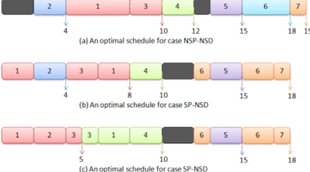
Figure 1: Optimal schedules for the three problems Figure 1 shows the optimal schedules for the three problems. In a production schedule, [j] means that the whole job j is produced. In a delivery schedule, [j] means that the whole job j is delivered. When [j] is preceded by a constant α, 0 < α < 1, this means that a part of job j is produced or delivered.
Case NSP-NSD: In the optimal schedule, the pro-duction sequence is ([2], [1], [3], [4], [5], [6], [7]). There exists an idle time before job 2, because if job 1 is processed before 2, then job 2 would be late. A sim-ilar reason for the second idle time holds. There are five delivery batches: {[2]}, {[1], [3]}, {[4]}, {[5]}, {[6]} and {[7]}, which depart respectively at time 4, 10, 12, 15, 18 and 19 as shown in Figure 1(a).
Case SP-NSD: The production sequence is (12[1], [2], [3],12[1], [4],13[6], [5], 23[6], [7]), where the job 1 and 6 are split respectively into two parts. The optimal schedule has four delivery batches: {[2]}, {[1], [3]}, {[4]}, {[5]} and {[6], [7]}, which depart respectively at time 4, 8, 10, 15 and 18 as shown in Figure 1(b). Since job 2 cannot be delivered with any other job because of its release time and deadline, transportation cost cannot be improved for the first 4 jobs with the non-splittable delivery. However, we can split job 6 in production in order to deliver the jobs 6 and 7 in one batch.
Case SP-SD: The production sequence is the same as problem SP-NSD. The optimal schedule has three full delivery batches: {12[1], [2],12[3]}, {12[3], 12[1], [4]}, {[5]} and {[6], [7]}, which depart respectively at time 5, 10, 15 and 18 as shown in Figure 1(c). For example, the first full filled delivery batch consists of half of job 1, job 2 and half of job 3. With the splittable delivery, the first four jobs can be delivered in two full batches.
Remark that in the three cases, jobs delivered to-gether are not necessarily sequenced consecutively, which makes the considered problems different from classical batching models.
1.3 RELATED LITERATURE
First, consider the production settings. Recall that the single machine scheduling problem with job re-lease dates and deadlines 1|rj, dj|− is NP-complete,
see (Garey and Johnson, 1979). (Carlier, 1982) pro-posed an efficient binary B&B algorithm to solve the corresponding optimization version 1|rj|Lmax, where
Lmax= maxj∈NLj= maxj∈N(Cj− dj). Here dj, j ∈
N, are no more deadlines, but due dates (i.e. they can be violated). When preemption is allowed, prob-lem 1|rj, pmtn|Lmaxcan be solved in polynomial time
O(n log n) using Jackson’s algorithm, see (Jackson, 1955).
It can be observed easily that problem 1|rj, dj|−
re-duces to our problem NSP-NSD, i.e. it is a special case of our problem with c = 1. Consequently, prob-lem NSP-NSD is NP-hard in the strong sense. When considering delivery, a similar model has been considered by Chen and Pundoor 2009 with the differ-ence that all the jobs are available for processing at time 0, i.e. rj = 0, j ∈ N , and the jobs may have
different sizes. The corresponding problem SP-SD is proved to be polynomially solvable in time O(n2).
The other problems (NSP-NSD and NSP-SD) are NP-hard in the strong sense. When the sizes of the jobs are all equal to one, the problem NSP-NSD is poly-nomially solvable in time O(n2log n), see (Pundoor and Chen, 2005).
When release dates are not all equal, to the best of our knowledge, only individual delivery to several cus-tomers is considered, i.e. c = 1. The objective is to minimize the maximum delivery time. Almost all considered problems in the literature are proved to be NP-hard, see for example (Chen, 2010) and (Liu and Cheng, 2002).
In this paper, we study in particular the problem NSP-NSD and propose a B&B algorithm to solve it optimally. This algorithm takes advantage of the bi-nary B&B algorithm proposed by (Carlier, 1982) and lower bounds on the transportation cost T C com-puted by solving special cases of problem SP-NSD. The paper is structured as follows. Section 2 consid-ers problems SP-SD and SP-NSD. Section 3 presents the B&B algorithm for the problem NSP-NSD fol-lowed, in section 4 by numerical experiments to eval-uate the performance of this algorithm. Finally, we provide conclusions and perspectives in section 5.
2 PROBLEMS SP-SD AND SP-NSD
In this section, we give some properties for problems SP-NSD and SP-SD. Then we provide a polynomial time algorithm that solves these problems in two spe-cial cases.
2.1 Properties
We introduce the definitions of production block and the preemptive EDD (earliest due date) rule, (Jack-son, 1955).
Definition 1 In a production schedule, a production block is defined as a subset of jobs which are processed consecutively without idle times. Set the minimum starting processing time of jobs of the block as the starting time of the block and the maximum comple-tion time of jobs of the block as the ending time of the block. The order of jobs is not taken into account in the definition of the block.
Preemptive EDD rule: At each decision point t in time, consisting of each release date and each job com-pletion time, schedule an available job j (i.e. rj ≤ t)
with the earliest due date. If no job is available at a decision point, schedule an idle time until the next release date.
Next, we give some properties for problems SP-NSD and SP-SD.
Lemma 1 If the problem is feasible, there exists an optimal integrated schedule for problems SP-NSD and SP-SD such that the following properties hold:
(1) Every job is processed in one production block only.
(2) Each production block starts at the minimum re-lease date of the jobs within this block.
Lemma 2 If the problem is feasible, there exists an optimal integrated schedule for problems SP-NSD and SP-SD such that the structure of production blocks, consisting of the jobs composition, the starting time and the ending time of each block, is the same as that constructed by the preemptive EDD rule.
2.2 A polynomial time algorithm for two spe-cial cases
We first introduce the Shortest Remaining Processing Time (SRPT) rule to construct a production schedule in the problems with preemption.
MOSIM14 - November 5-7-2014 - Nancy - France
SRPT rule: at each decision point t in time, con-sisting of each release date and each job completion time, schedule an available job j (i.e. rj ≤ t) with
the shortest remaining processing time. If no job is available at a decision point, schedule an idle time until the next release date.
Next, we provide a polynomial time algorithm (see Algorithm A1) for problems SP-NSD and SP-SD in the following two special cases:
case 1: the truck capacity is unlimited, i.e. c = ∞. case 2: In any production block of the schedule
con-structed by preemptive EDD rule, the jobs have the same release date.
Algorithm A1
Step 1: Generate a production schedule σ with the preemptive EDD rule. If Cj(σ) ≤ dj, ∀j ∈ N
go to Step 2, otherwise there is no solution and STOP.
Step 2: Let N0 ⊆ N denote the set of undeliv-ered jobs. Set current delivery time T = maxj∈N0Cj(σ).
Step 3: Find the set of undelivered jobs with the deadline greater than or equal to T . Let S denote this jobs’ set.
Step 4: If |S| ≤ c, deliver the jobs of S in one batch which departs at time T . Otherwise, reschedule the jobs of S in σ with the SRPT rule and do not change the schedule of the other jobs, then deliver the last completed c jobs of S in one batch which departs at time T . If all jobs are delivered, then STOP. Otherwise, go to step 2.
Theorem 1 Algorithm A1 finds an optimal inte-grated schedule for problems SP-NSD and SP-SD in the special case 1 in O(n2) time, and the special case
2 in O(n2log n) time.
Remark that the computational complexity of prob-lems SP-NSD and SP-SD in the general case is still open.
3 A B&B ALGORITHM FOR PROBLEM NSP-NSD
As it has been observed in section 1, the problem NSP-NSD is strongly NP-hard. In this section, we first present two heuristics to determine upper bounds on T C. Then we describe a B&B algorithm to solve our problem.
3.1 Heuristics
We first propose a polynomial time algorithm (see algorithm A2) to construct an optimal delivery schedule for a given feasible non-preemptive produc-tion schedule σ, i.e. Cj(σ) ≤ dj, ∀j ∈ N .
Algorithm A2
Step 1: Let N0 ⊆ N denote the set of undeliv-ered jobs. Set current delivery time T = maxj∈N0Cj(σ).
Step 2: Find the set of undelivered jobs with the deadline greater than or equal to T . Let S denote this jobs set.
Step 3: If |S| ≤ c, deliver all jobs of S in one batch which departs at time T . Otherwise, deliver the last c completed jobs of S in one delivery batch which departs at time T . If all jobs are delivered, then STOP. Otherwise, go to Step 1.
This algorithm can be used to determine an upper bound of T C for a given production schedule without preemption. In our B&B algorithm, we will use two heuristics that try to construct a feasible integrated schedule for problem NSP-NSD.
The first heuristic, denoted H1, uses the non-preemptive EDD rule, which forces to create a production schedule without preemption. If the obtained production sequence is feasible, then we apply algorithm A2.
Non-preemptive EDD rule: At each decision point t in time, consisting of each starting of a production block and each job completion time, schedule an available job j (i.e. rj ≤ t) with the earliest due date.
If no job is available at a decision point, schedule an idle time until the next release date.
The second heuristic, denoted H2, uses a feasible SP-NSD integrated schedule to construct, if possible, a feasible integrated schedule for problem NSP-NSD.
Heuristic H2
Step 1: Create a priority list of jobs, such that in the given schedule, if Di< Dj, job i must be before
job j in the list, and if Di = Dj and Ci < Cj,
Step 2: Schedule each job as early as possible with-out preemption. When there are several jobs which can be scheduled, we choose the job with the highest priority. Let σ be the constructed schedule. If Cj(σ) ≤ dj, ∀j ∈ N , go to step
3. Otherwise, there is no feasible solution and STOP.
Step 3: Apply the algorithm A2 to compute a deliv-ery schedule.
3.2 B&B algorithm
We recall the B&B algorithm by (Carlier, 1982) for problem 1|rj|Lmax. The algorithm computes a lower
bound and an upper bound for each node based on preemptive and non-preemptive EDD rule, respec-tively. Branching is done by modifying release times or deadlines. At every node, the algorithm constructs the non-preemptive EDD schedule, then defines a critical job and a critical set of jobs and considers two subsets of schedules: the schedules where the critical job precedes the jobs of the critical set and the sched-ules where the critical job follows the jobs of critical set.
We propose a B&B algorithm (see Algorithm B2) for problem NSP-NSD based on the B&B algorithm of Carlier. Let LB(Lmax, u) and U B(Lmax, u) denote
the lower bound of Lmax and the lower bound of
Lmax of node u respectively. Let LB(T C, u) and
U B(T C, u) denote the lower bound of T C and the upper bound of T C of node u respectively. Let U B∗(T C) denote the current best upper bound of T C. The algorithm B2 uses the same branching as Carlier’s algorithm. When a feasible solution is found at node u, we apply another B&B algorithm from the node u to try to find a local optimal solution for T C. Branching of B1 is done by assigning at each position of the schedule a job respecting a set of rules (see algorithm B1). When algorithm B1 stops, algorithm B2 continues the branching for the remaining active nodes.
Algorithm B1
Lower bound: we solve two relaxed problems, each respecting one of the two special cases of prob-lem SP-NSD by applying the algorithm A1. Let (σ1, θ1) and (σ2, θ2) denote the obtained
SP-NSD integrated schedules. Set LB(T C) = max{T C(σ1, θ1), T C(σ2, θ2)}.
Upper bound: Firstly, generate two integrated schedules for problem NSP-NSD with the two above obtained schedules (σ1, θ1) and (σ2, θ2) as
input by applying the heuristic H2. Secondly,
generate a third integrated schedule by apply-ing the heuristic H1. Finally, if one or several constructed integrated schedules are feasible, set U B(T C) as the smallest T C among these sched-ules. Otherwise, set U B(T C) = n + 1. Update U B∗(T C) if necessary.
Branching: if LB(T C, u) < U B∗(T C, u) for a node u, firstly choose one job to be scheduled in the current position. A job j is candidate if it re-spects the following three rules. Let N0 denote the set of unscheduled jobs without job j. active scheduling rule: rj < mink∈N0(rk +
pk)
deadline rule: rj+ pj≤ mink∈N0(dk− pk)
precedence relations rule: P
k∈N0xkj = 0,
where xkj = 1 if the job k precedes the job
j, otherwise xkj= 0.
Then, require the candidate j to be scheduled at the current position by setting rk = max(rk, rj+
pj), ∀k ∈ N0.
Algorithm 1: Algorithm B2
1 Generate the root associated with LB(Lmax, root)
and U B(Lmax, root) as the algorithm of Carlier, and
put this node in list L;
2 while L 6= ∅ do
3 Choose one node u in L with minimum
LB(Lmax, u) ;
4 if U B(Lmax, u) > 0 and LB(Lmax, u) ≤ 0 then 5 Generate LB(T C, u) and U B(T C, u) using
algorithm B1 ;
6 if LB(T C, u) < U B∗(T C) then 7 if U B(T C, u) < n + 1 then
8 Apply algorithm B1 with the original
pj and dj, the modified rj of node u,
and the precedence relations between jobs imposed at the path from the root to the node u;
9 else
10 Branch as the algorithm of Carlier
and add new nodes with the bounds of Lmax in L;
11 else
12 if LB(Lmax, u) ≤ U B(Lmax, u) ≤ 0 then 13 Apply algorithm B1 with the original pj
and dj, the modified rj of node u, and
the precedence relations between jobs imposed at the path from the root to the node u;
MOSIM14 - November 5-7-2014 - Nancy - France
4 Experimental results
We evaluate the performance of the B&B algorithm B1 by comparing it with an ILP (integer linear pro-gramming) model for the problem NSP-NSD. The B&B algorithm B1 was implemented in C++ and the ILP was implemented in Cplex V12.5.1. The experi-ments were carried out on a DELL 2.50GHz personal computer with 8GB RAM. The ILP model extends the well-known disjunctive scheduling model as fol-lows. Suppose that each batch departs at one dead-line, and let s1, . . . , su denote the possible departure
dates. Let M be a sufficiently large number.
Decision variables:
• xij =
1, if job i precedes job j, i = 1, . . . , n, j = 1, . . . , n
0, otherwise
• tj= production starting time of job j,
j = 1, . . . , n
• yiq=
1, if job i is delivered at time sq,
i = 1, . . . , n, q = 1, . . . , u 0, otherwise
• wq = number of batches departing at time sq,
q = 1, . . . , u ILP: min u X q=1 wq (1) s.t. tj− ti ≥ pi− (1 − xij)M, i, j = 1, . . . , n(2) xij+ xji= 1, i, j = 1, . . . , n, i 6= j (3) tj ≥ rj, j = 1, . . . , n (4) tj+ pj≤ u X q=1 (yiqsq), j = 1, . . . , n (5) n X i=1 yiq≤ cwq, q = 1, . . . , u (6) u X q=1 yiq= 1, i = 1, . . . , n (7) yiq= 0, if di< sq, i = 1, . . . , n, q = 1, . . . u(8) xij∈ {0, 1}, i = 1, . . . , n, j = 1, . . . , n (9) yiq∈ {0, 1}, i = 1, . . . , n, q = 1, . . . , u (10) wq∈ N, q = 1, . . . , u (11)
In the ILP model, the objective function is to mini-mize the number of delivery batches. Constraints 2 ensure that, in the production schedule, job j starts
after the completion of job i if job i precedes job j. Constraints 3 guarantee that, in the production schedule, either job i precedes job j or job j precedes job i for any two different jobs i and j. Constraints 4 guarantee that, in the production schedule, each job starts after its release date. Constraints 5 ensure that each job is delivered after its production com-pletion time. Constraints 6 are the constraints of the truck capacity. Constraints 7 ensure that each job is delivered in one batch only. Constraints 8 are the constraints of the delivery deadline. Constraints (9) – (11) give the domain of definition of each variable. We reuse the method of (Briand et al., 2010) to generate data for problem NSP-NSD. We consider n ∈ {10, 20, 30, 50, 70, 100, 150, 200, 300, 500}. The integers pj, rj and dj are generated respectively
from the uniform distribution [1,50], [0, αPn
j=1pj] and [(1 − β)aPn j=1pj, a Pn j=1pj], where α, β ∈ {0.2, 0.4, 0.6, 0.8, 1} and a ∈ {100%, 100%}. If dj <
rj+ pj, dj has been updated by rj+ pj. We choose
a set of hard instances and test them with the B&B algorithm of Carlier to find the minimum Lmax. This
value is added to each dj to ensure that we have at
least one feasible solution. For n ≤ 100, we con-sider the batch capacity c ∈ {2, 3, dn8e, dn
4e}, and c ∈ {d50ne, dn 30e, d n 20e, d n
10e} for n > 100. A total
num-ber of 554 instances is obtained.
B&B algorithm
n Fea Opt Node Time
10 100% 100% 0 0.05 20 100% 100% 5 0.38 30 100% 97.5% 72 7.72 50 100% 90.00% 255 33.99 70 100% 87.50% 307 56.22 100 100% 80.00% 372 85.08 150 100% 51.19% 368 161.24 200 100% 62.50% 230 125.81 300 97.62% 46.43% 199 184.43 500 70.83% 12.50% 156 289.68 Table 2: Performance of the B&B algorithm. The Tables 2-5 illustrate the performance of the B&B algorithm and the ILP model. When imposing 5 min-utes as the limit of execution time, we use the follow-ing measures to compare the B&B algorithm and the ILP model.
Fea: the percentage of instances for which a feasi-ble solution is determined within the given time limit.
Opt: the percentage of instances which are solved to optimality within the given time limit.
ILP
n Fea Opt Node Time 10 100% 73% 684726 102.43 20 100% 100% 9840 3.57 30 97.5% 85% 49955 50.02 50 40% 32.5% 41059 224.35 70 - - - -100 - - - -150 - - - -200 - - - -300 - - - -500 - - -
-Table 3: Performance of the ILP model.
B&B algorithm
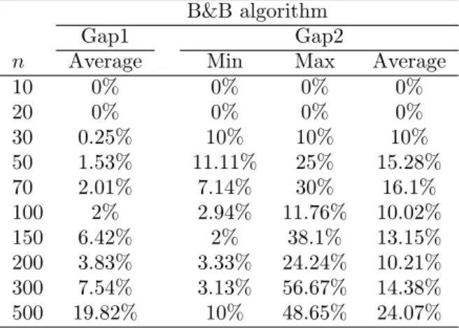
Gap1 Gap2
n Average Min Max Average
10 0% 0% 0% 0% 20 0% 0% 0% 0% 30 0.25% 10% 10% 10% 50 1.53% 11.11% 25% 15.28% 70 2.01% 7.14% 30% 16.1% 100 2% 2.94% 11.76% 10.02% 150 6.42% 2% 38.1% 13.15% 200 3.83% 3.33% 24.24% 10.21% 300 7.54% 3.13% 56.67% 14.38% 500 19.82% 10% 48.65% 24.07%
Table 4: Gaps for the B&B algorithm.
Time: the average CPU time in seconds.
Gap1: the relative gap measured by (U B∗(T C) − LB∗(T C))/LB∗(T C), where U B∗(T C) and
LB∗(T C) are the best upper bound and lower bound at the end of the algorithm. We consider the instances for which we obtained at least one feasible solution (optimal solution included). Gap2: the relative gap for the instances for which we
obtained at least one feasible solution (optimal solution excluded).
The results show that the B&B algorithm outper-forms the ILP model. Remark that the average ex-ecution time and the number of nodes with the ILP model are always larger than the B&B algorithm, and the ILP model cannot find a feasible solution with n ≥ 70 within 5 minutes as time limit. Consulting the gaps, we observe that the B&B algorithm has a much better performance. Besides, the B&B algo-rithm solves all the instances with n ≤ 20 optimally within a very short execution time less than one sec-ond, and more than 80% of the instances with n ≤ 100 optimally within an average execution time less than
ILP
Gap1 Gap2
n Average Min Max Average 10 6.6% 16.67% 44.44% 24.43% 20 0% 0% 0% 0% 30 1.83% 9.09% 27.27% 14.24% 50 6.51% 13.33% 50.43% 34.75% 70 - - - -100 - - - -150 - - - -200 - - - -300 - - - -500 - - -
-Table 5: Gaps for the ILP model.
100 seconds. The B&B algorithm finds at least a fea-sible solution with n up to 200 and 5 minutes as time limit. In average, the Gap1 and the Gap2 of the B&B algorithm are less than 8% and 16% when n ≤ 300. However, the maximum Gap2 shows some hard cases. 5 Conclusion
In this paper, we study an integrated production and outbound distribution scheduling problem with one manufacturer and one customer. We provide a poly-nomial time algorithm for two special cases of prob-lems SP-NSD and SP-SD. We also provide a B&B algorithm for the problem NSP-NSD and evaluate its performance using numerical experiments. The re-sults show that the proposed algorithm has the better performance than the ILP model and can solve opti-mally more than 80% of the instances with n ≤ 100 within an average execution time less than 100 sec-onds.
Several important research issues remain open for fu-ture investigations. A first important research direc-tion is to study the complexity of problems SP-NSD and SP-SD. Another issue is to provide a better lower bound for the B&B algorithm. Finally, one might consider extending the model to a production system with parallel machines.
ACKNOWLEDGMENTS
This project was partly funded by ANR (BLANC pro-gram 2013 ”ATHENA” project)
References
[1] C. Briand, S. Ourari, and B. Bouzouia. An efficient ilp formulation for the single machine scheduling problem. RAIRO - Operations Re-search, 44:61–71, 2010.
MOSIM14 - November 5-7-2014 - Nancy - France
[2] J. Carlier. The one-machine sequencing prob-lem. European Journal of Operational Research, 11(1):42–47, 1982.
[3] Z.-L. Chen. Integrated production and outbound distribution scheduling: Review and extensions. Operations Research, 58(1):130–148, 2010. [4] Z.-L. Chen and G. Pundoor. Integrated order
scheduling and packing. Production and Opera-tions Management, 18(6):672–692, 2009.
[5] Z.-L. Chen and G. L. Vairaktarakis. Integrated scheduling of production and distribution op-erations. Management Science, 51(4):614–628, 2005.
[6] S. S. Ereng¨u¸c, N. C. Simpson, and A. J. Vakharia. Integrated production/distribution planning in supply chains: An invited re-view. European Journal of Operational Research, 115(2):219–236, 1999.
[7] M. Garey and D. Johnson. Computers and Intractability: A Guide to the Theory of NP-Completeness. W.H. Freeman, 1979.
[8] N. G. Hall and C. N. Potts. Supply chain scheduling: Batching and delivery. Operations Research, 51(4):566–584, 2003.
[9] J. R. Jackson. Scheduling a production line to minimize maximum tardiness. Technical report, University of California, Los Angeles, 1955. [10] Z. Liu and T. Cheng. Scheduling with job release
dates, delivery times and preemption penalties. Information Processing Letters, 82(2):107 – 111, 2002.
[11] A. M. Sarmiento and R. Nagiy. A review of in-tegrated analysis of production-distribution sys-tems. IIE Transactions, 31(11):1061–1074, 1999. [12] D. J. Thomas and P. M. Griffin. Coordinated supply chain management. European Journal of Operational Research, 94:1–15, 1996.