HAL Id: inserm-00910761
https://www.hal.inserm.fr/inserm-00910761
Submitted on 28 Nov 2013
HAL is a multi-disciplinary open access
archive for the deposit and dissemination of sci-entific research documents, whether they are pub-lished or not. The documents may come from teaching and research institutions in France or abroad, or from public or private research centers.
L’archive ouverte pluridisciplinaire HAL, est destinée au dépôt et à la diffusion de documents scientifiques de niveau recherche, publiés ou non, émanant des établissements d’enseignement et de recherche français ou étrangers, des laboratoires publics ou privés.
MULTI-ATLAS-BASED SEGMENTATION OF
PELVIC STRUCTURES FROM CT SCANS FOR
PLANNING IN PROSTATE CANCER
RADIOTHERAPY
Oscar Acosta, Jason Dowling, Gael Drean, Antoine Simon, Renaud de
Crevoisier, Pascal Haigron
To cite this version:
Oscar Acosta, Jason Dowling, Gael Drean, Antoine Simon, Renaud de Crevoisier, et al.. MULTI-ATLAS-BASED SEGMENTATION OF PELVIC STRUCTURES FROM CT SCANS FOR PLAN-NING IN PROSTATE CANCER RADIOTHERAPY. Ayman S. El-Baz; Luca Saba; Jasjit Suri. Abdomen and Thoracic Imaging, Springer US, pp.623-656, 2013, �10.1007/978-1-4614-8498-1_24�. �inserm-00910761�
Abdomen And Thoracic Imaging, 2014, pp 623-656
MULTI-ATLAS-BASED SEGMENTATION OF
PELVIC STRUCTURES FROM CT SCANS FOR
PLANNING IN PROSTATE CANCER
RADIOTHERAPY
Oscar Acosta (oscar.acosta@univ-rennes1.fr) (4) (5), Jason Dowling (6), Gael Drean (4) (5), Antoine Simon (4) (5), Renaud de Crevoisier (4) (5) (7), Pascal Haigron (4) (5)
4. INSERM, U1099, Rennes, 35000, France
5. Université de Rennes 1, LTSI, Rennes, 35000, France
6. The Australian e-Health Research Center-CSIRO, Brisbane, Australia
7. Département de Radiothérapie, Centre Eugène Marquis, Rennes, 35000, France
Abstract
In prostate cancer radiotherapy, the accurate identification of the prostate and organs at risk in planning computer tomography (CT) images is an important part of the therapy planning and optimization. Manually contouring these organs can be a time consuming process and subject to intra- and inter-expert variability. Automatic identification of organ boundaries from these images is challenging due to the poor soft tissue contrast. Atlas-based approaches may provide a priori structural information by propagating manual expert delineations to a new individual space; however the inter-individual variability and registration errors may lead to biased results. Multi-atlas approaches can partly overcome some of these difficulties by selecting the most similar atlases among a large data base but the definition of similarity measure between the available atlases and the query individual has still to be addressed. The purpose of this chapter is to explain atlas-based segmentation approaches and the evaluation of different atlas-based strategies to simultaneously segment prostate, bladder and rectum from CT images. A comparison between single and multiple atlases is performed. Experiments on atlas ranking, selection strategies and fusion decision rules are carried out to illustrate the presented methodology. Propagation of labels using two registration strategies are applied and the results of the comparison with manual delineations are reported.
1. Introduction
Prostate cancer is one of the most commonly diagnosed male cancer worldwide[1], with 190,000 new cases diagnosed in USA in 2010 [2] and 71,000 new cases in France in 2011 [3]. In Australia, prostate cancer is the most commonly diagnosed cancer behind skin cancer, and is the second highest cause of cancer-related deaths behind lung cancer [4]. External beam radiation therapy (EBRT) is a major clinical treatment for prostate cancer which has proven to be efficient for tumor control [5]. EBRT uses high energy x-ray beams combined from multiple directions to deposit energy (dose) within the patient tumor region (the prostate) to destroy the cancer cells. Modern treatment techniques offer nowadays improved treatment accuracy through a better planning, delivery, visualization and the correction of patient setup errors .
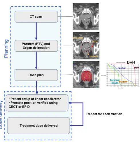
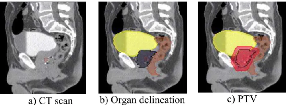
The standard clinical protocol for EBRT treatment planning is shown in Figure 1. During the planning step, CT images from patients are acquired. The treatment targets (prostate and potentially seminal vesicles) along with important normal tissues (rectum, bladder, and femoral heads) are manually delineated using the scans. If MRI is used for the prostate definition then alignment of the MRI and the CT is performed to transfer the MRI structure contours to the CT scan. A defined prostate volume is then expanded to constitute the Planning Target Volume (PTV) for treatment (Figure 2). These spatial margins between the organs and the PTV allow for uncertainties in delineation, patient setup, motion and organ deformations [6] [7] [8].
The next step is the use of computer planning tools to determine the directions, strengths, and shapes of the treatment beams which will be used to deliver a prescribed dose to the defined target while
minimizing the dose to the normal tissues, according to a certain number of recommendations (eg.[9]). Thus, a treatment plan consists of dose distribution information over a 3D matrix of points overlaid onto the individual's anatomy. Dose volume histograms (DVHs) summarize the information contained in the 3D dose distribution and may serve as tools for quantitative evaluation of treatment plans. The International Commission on Radiation Units and Measurements (ICRU) 50 and 62 reports define and describe several target and critical structure volumes that aid in the treatment planning process and that provide a basis for comparison of treatment outcomes. For example, to comply with ICRU recommendations for prostate, 95% of the PTV is irradiated with at least 95% of the prescribed dose. For the rectal wall the maximal dose should be less or equal than 76Gy and the irradiated volume at 72Gy, must be less than 25%. Finally, during the dose delivery step, which may last several weeks, the patient is carefully positioned at the accelerator and the treatment is performed according to the planning. A frequent method to align the patient for treatment is to use small implanted fiducial markers in the prostate. These are visible under x-ray imaging and show precise prostate position within the body. Image guidance may be used to align the treatment target each day for the entire course.
Figure 1. Workflow for traditional prostate cancer image guided radiation therapy. The prescribed radiation dose for EBRT is generally delivered over
a) CT scan b) Organ delineation c) PTV
Figure 2. Sagittal views of CT scan delineation and definition of the Planned Target Volume (PTV).
Figure 3. Typical Intensity Modulated Radiation Therapy (IMRT) plan (axial, coronal and sagittal views) showing iso-dose curves and the (PTV), obtained
after organ delineations.
One of the main challenges in prostate radiotherapy is to control the tumor, by accurately targeting the prostate, while sparing neighboring organs at risk (bladder and rectum). Several strategies have been developed in order to improve local control, particularly by increasing the radiation dose with highly conformal techniques demonstrating a strong dose-effect relationship [10]. The precision of treatment delivery is steadily improving due to the combination of intensity
modulated RT (IMRT) and image-guided RT (IGRT) and intraprostatic fiducial markers. New delivery systems are also populating clinical centers (ARC-Therapy, cyberknife). Hence the possibilities for achieving better control by increasing the dose are within reach. However, dose escalation is limited by rectal and urinary toxicity ([11], [12]). Toxicity events (incontinence, rectal bleeding, stool lose) are frequent with standard prescribed doses (70 -80 Gy) and may even significantly increase for higher doses [13]. Thus, accurate delineation of both prostate and organs at risk (OARs) (i.e. bladder, rectum) from planning images are crucial to exploit the new capabilities of the delivery systems [14]. Identifying the boundaries of pelvic structures are of major importance not only at the planning step but also in other radiotherapy stages such as patient setup correction, accumulating dose computation when IGRT is used [15] [16] or for toxicity population studies [17].
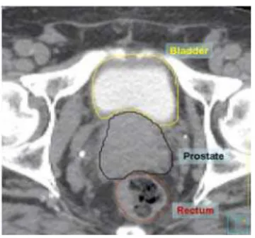
Figure 4. Axial view of manual segmentation of bladder, prostate and rectum overlaid on CT scan.
Nowadays, the organ contouring tasks are mainly carried out manually by medical experts. However, the CT offers poor soft tissue contrast and therefore segmenting pelvic organs is highly time consuming (between 20-40 minutes to delineate each). Manual contouring requires training and is prone to errors, especially in the apical and
basis regions [18] [19]. These uncertainties lead to large intra- and inter-observer variation [20] and may impact treatment planning and dosimetry [19] [21]. Previous studies, for instance, have reported a prostate delineation variance of 20:60% [20]. For the rectum and bladder this difference may be as high as 2.5 to 3% [22]. Although improved organ contrast may be obtained with Magnetic Resonance Images (MRI), and several studies are in progress to introduce MRI in the radiotherapy planning ([23], [24]), CT scans are still required to perform this task since dose computation relies on electron density. Therefore there is a strong case for more reliable semi or fully automatic CT segmentation techniques. When dealing with automatic segmentation methods for prostate cancer treatment there are several difficulties which may arise. Firstly, there is a poor contrast between prostate, bladder and rectum and, secondly, there may exist a high variability in the amount of bladder and rectum filling. These challenges restrict the use of classical intensity-based segmentation methods. In addition the high intra- and inter-individual variability may cause model-based methods to fail [25].
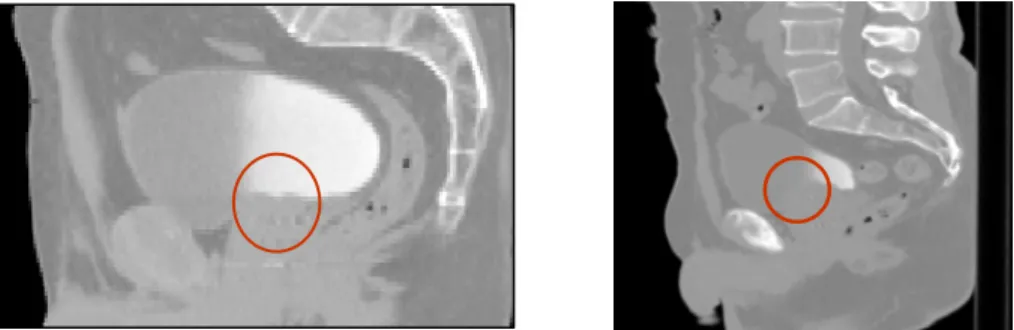
Figure 5. Two examples of pelvic structures in CT (sagittal views). The poor contrast between structures hampers organ segmentation.
Atlas based approaches are common methods for organ segmentation, not only for obtaining a final contour but also to provide initial organ positions for further segmentation algorithms. In atlas-based methods a pre-computed segmentation or prior information in a template space is propagated towards the image to be segmented via spatial normalization (registration). These methods have been largely used in brain MRI ( [26], [27] ), head and neck CT Scans ( [28], [29], [30] ), cardiac aortic CT [31], pulmonary lobes from CT [32] and prostate MR ( [33], [34] ) . In the atlas based methods image registration is a key element, as label propagation relies on the registration of one or more templates to a target image.
In this chapter a brief overview of image registration and atlas methods will be provided. Atlas based methods which can perform the segmentation of the individuals' pelvic structures, prostate and organs at risk (OAR) from CT scans will be discussed and evaluated against clinical datasets.
2. Image registration
2.1 Introduction
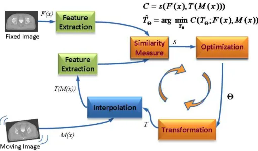
Atlas based segmentation is heavily dependent on the quality of image registration. Medical image registration involves determining the spatial transform which maps points from a moving image to homologous points on a object in a fixed image. The general idea of the registration may be summarized as in Figure 6.
The basic input data to the registration process are two images: one is defined as the fixed image F(X) and the other as the moving image
M(X). The output of the registration is a spatial transformation T
allowing the warping or the alignment of the moving image, on the fixed image, according to a similarity metric.
Figure 6. Computerized registration framework.
As depicted in Figure 6, there are four main components involved in image registration: a similarity measure between two images; the transformation model used to map points between images; a method to find the optimal transform parameters; and finally an interpolator to calculate moving image intensities at non-grid positions [20].
In this sense, registration may be seen as an optimization problem )) ( ), ( ; ( min arg ˆ C T F x M x T T (1)
aimed at estimating the spatial mapping that better align the moving image into alignment with the fixed image according to a cost function: ))) ( ( ), ( (F x T M x s C (2)
where is the similarity criterion, which provides a measure of how well the fixed image is matched by the transformed moving image. This measure forms the quantitative criterion to be optimized over the search space defined by the parameters of the transform. The similarity may lie on control points, features, anatomical structures, intensities, etc. Here, we restricted the study to the intensity similarity metrics.
)) ( ( ), ( (F x T M x s 2.2 Transform
The transform component T(X) represents the spatial mapping of points from the fixed image space to points in the moving image space. The transformation model can either apply to the entire volume (global) or to each voxel (local).
The two global methods are: rigid registration which allows only rotations and translations; and affine registration which extends rigid registration with the addition of skew and scaling parameters.
Deformable, (also known as non-rigid or non-linear) registration affects individual voxels within the volume. This enables the matching of soft tissues which may deform between scans (eg. a patient’s bladder on two CBCT volumes) or when performing inter-individual mapping. Typically a regularization constraint is also implemented to constrain the allowable solution space. Deformable
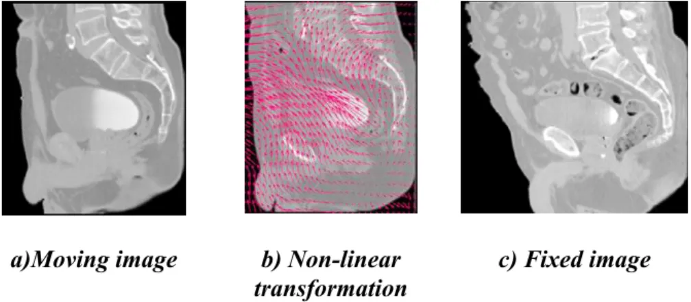
methods can be complex and difficult to validate [35]. Common deformable transforms include BSpline free form deformation (FFD) [36], thin plate splines [37], and optical flow inspired approaches (Demons algorithm) [38]. The output from deformable registration is generally a volume (the deformation field) which contains displacement vectors for each voxel as illustrated in Figure 7
a)Moving image b) Non-linear transformation
c) Fixed image
Figure 7. Example of a non-linear transformation obtained when registering the moving image (a) into the espace of the fixed image (b).
2.2 Image similarity metrics
When the similarity between two images is based on intensity levels, several metrics can be considered [39] These can be computed via their voxel-wise differences, for example with the sum of squared differences (SSD), or via the cross correlation (CC) or the mutual information (MI). These metrics are computed as follows:
(3)
i i i T M x x F n SSD 1 ( ( ) ( ( )))2where is the fixed image and represents the transformed moving image. The CC as
) (xi F T(M(xi))
i i i i i i i x M T x M T x F x F x M T x M T x F x F CC 2 2 ))) ( ( )) ( ( ( )) ( ) ( ( ))) ( ( )) ( ( ))( ( ) ( ( (4)and the MI, computed as
) , ( ) ( ) ( ) , (F M H F H M H F M MI (5)
where H(x) is the individual entropy of an image x, given by
) ( log ) ( ) (F p i p i H i
(6) and ) , ( log ) , ( ) , (F M , p i j p i j H
ij (7)is the joint entropy and p the joint probability. The idea behind the term −H(F, M), is that maximizing MI is related to minimizing joint entropy. A more robust version of the MI is the normalized mutual information (NMI) proposed by Studholme, et al. [40], and computed as ) , ( ) ( ) ( ) , ( M F H M H F H M F NMI (8)
An important consideration with similarity metrics is the computational cost and the need of a large number of samples for the algorithms to be robust. Novel ways of computing MI, have been proposed [41], yielding comparable results with less samples. This approach approximates the entropy computation using the high order description. For a complete survey of MI, the reader may refer to [42].
2.3 Optimization
The images (or image features), are ideally related to each other by some transformation T. As shown in Figure 6, the iterative process of optimization aims at finding T with a cost function determined by the similarity metric. As the cost function may have multiple local minima, a weighted regularization term may be added to penalize undesirable deformations as
s F x T M x w
C ( ( ), ( ( ))) (9)
Examples of include the curvature, the elastic energy, or volume preserving constraints. This term ensure smoothness of T in the non-parametric approaches. There are several ways to perform the optimization of T. These include the deterministic gradient-based algorithms such as gradient-descent, quasi-Newton or non-linear
gradient descent; or the stochastic gradient-based algorithms such as the Kiefer-Wolfowitz, simultaneous perturbation; Robins Monro and Evolution Strategy, where they derive search directions with stochastic approximations of the derivative.
A full evaluation of optimization techniques in a non-rigid registration context was presented by Klein, et al. [33]. They compared several methods with respect to speed, accuracy, precision and robustness. By using a set of CT images of heart and MR images of prostate, it was shown that a stochastic gradient descent technique the Robins-Monro process outperformed the other approaches. Acceleration factors of approximately 500, compared to a basic gradient descent method were achieved.
2.4 Interpolation
As depicted in Figure 6, after a transformation is applied to the moving image, an interpolation is performed which enables evaluation of the moving image intensities at non-grid positions. To resample the moving image in the fixed image grid, the transformation can be applied either in a forward or backward manner. In the forward way, each voxel from the moving image can be directly transformed using the estimated mapping functions. Because of the discretization, this approach can produce holes and/or overlaps in the transformed image. Hence, the backward approach is more convenient and usually implemented. In this approach, the image interpolation takes place on the regular grid in the space of the fixed image. Thus, the registered image data from the moving image are determined using the coordinates of the target voxel and the inverse of the estimated transformation. In this way, neither holes nor overlaps can occur in the output image. Thus, depending on the required precision different alternatives exist for this resampling, for instance the nearest neighbor
(NN), tri-linear, BSpline (BS), Cubic interpolations (CI), etc. However, some artefacts may be introduced as a consequence of the iterative process. These interpolation-related errors in image registration have been studied by Pluim, et al. [43] . Thevenaz, et al. [44] have proposed a different approach to image resampling. Unlike the other methods, their resampling functions do not necessarily interpolate the image gray levels but values calculated as certain functions of the gray levels. The authors demonstrated how this approach outperforms traditional interpolation techniques. Several survey papers on resampling techniques have been published recently ([45], [46], [47], [48]).
In practical terms, although higher-order methods may yield good result in terms of accuracy, the tri-linear interpolation offers a very good trade-off between accuracy and computational complexity. Cubic or spline interpolation is recommended when the transformation involves significant geometrical differences, as several voxels may be interpolated in between available information. Nearest neighbor interpolation produces several artefacts but is advised when the image to be transformed contains low number of intensities. For example, when propagating labels in atlas-based segmentation approaches, this is the preferred approach.
3. General atlas construction and segmentation strategies
3.1 Introduction
The key idea in atlas-based segmentation is to use image registration to map one or more pre-labeled images (or “atlas”) onto a new patient image. Once a good correspondence between structurally equivalent regions in the two images is achieved the labels defined on
the atlas can be propagated to the image. Rohlfing, et al. [49] have identified four main methods to generate the atlas which is registered to a target volume: using a single labeled image, generating an average shape image, selecting the most similar image from a database of scans; or finally to register all individual scans from a database and using multi-classier fusion to combine the pair-wise registration results.
An atlas A is constituted by a template image i I and, a set of i generated labels i defined in the same coordinate system. In the case of pelvic structures from CT scans, the set of labels
i{prostate,rectum,bladder}
. The general framework of
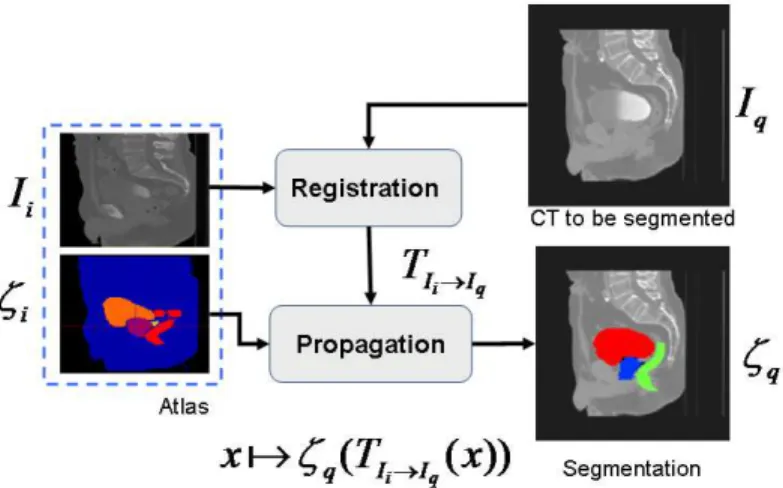
atlas-based segmentation, as depicted in Figure 8, relies on the registration of the template , to the query image in order to obtain a transformation q i I I , that maps i i I T q I
into q . If the mapping is anatomically correct, the yielded segmentation is accurate and anatomically meaningful. It is worth nothing that the similarity between the images I and i q, as explained in previous sections may impact the registration results and therefore the segmentation.
I
Figure 8. Atlas Based Segmentation Strategy
Several issues may arise under this framework in order to produce accurate segmentations. Firstly, the selection and generation of the initial patient scan which may be representative of a population; secondly, the registration strategy to bring into the space of ; and finally, the propagation of the labels
i
I Iq
i
into .and the subsequent generation of the new segmentation
q
I
q
.
Concerning the first issue, a typical individual from a given population may constitute an atlas, where the segmentation i may be manually generated on I . This is the simplest strategy, but with the problems i related to the inter-individual variability and inter-observer rating arising. However, in order to attenuate the dependency on a single observer, a group of experts can generate the set of labels, adding robustness to the definition of i. To a larger extent, to cope with the inter-individual variability, several individuals from a population can be used to constitute the atlas. In this case, two kinds of strategies may be followed. Either an atlas is built from the population by averaging the data ( Ii , i i0,..,M ) or alternatively each individual is
considered as a single atlas. In that case, for a given query, there is a previous selection of the best n atlasesAi, i0,..,M which better fit to the query q. The last strategy allows for a reduction of the bias inherent to using a single template, but new questions arise concerning the best atlas selection strategy and label fusion decisions to constitute the final segmentation q
I
. These points are detailed in the following sections. Proposed experiments compare the performances of those for segmenting prostate, bladder and rectum.
3.2 Average atlas construction
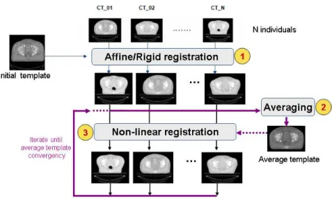
An atlas can be computed in an iterative process as depicted in Figure 9. This approach was used in a comparative study that we presented in [17], but also is detailed in [50]. In this scheme, an arbitrary but representative individual was chosen as the initial template, defining the atlas space alignment. The first iteration involves the registration of every other individual to the selected template using a rigid or affine registration method (i.e. robust block matching approach [51], followed by a non-rigid registration [38] in the subsequent iterations. At the end of each iteration, a new average atlas is generated and used in the subsequent iteration.
Figure 9. Iterative averaging for obtaining a template
After the average template is obtained, a probabilistic set of soft labels
i
(probability maps) is eventually generated by propagating the manual segmentations of these organs for each case using the obtained affine transform and deformation field into the atlas space. Figure 10 shows the obtained template after five iterations and Figure 11, depicts an overlaid of the probabilistic labeling for the prostate in the atlas coordinate system.
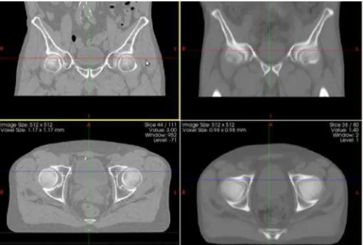
Figure 10. Example of a) Individual's CT and b) Averaged template
The drawbacks of this strategy within the context of CT pelvic segmentation come from the large inter-individual variability and the poorly contrasted average atlas which is produced after several iterations. In order to diminish the bias inherent to using a single template, one potential strategy is to select one patient amongst typical individuals from a database, who is quite similar to the majority of individuals. Additional benefits may be brought to the segmentation by combining the results from multiple atlases, improving the accuracy as explained in the next section.
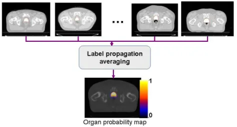
Figure 11. Generation of organ probability maps by propagating labels into the common template
3.3 Multi-atlas strategy: selecting the N best atlas from a database
Previous works have shown the benefits to combine multiple atlases (multi-atlases-based approaches), improving the segmentation accuracy (eg. [26], [31], [27], [52] ). Thus, given a query individual, different possibilities appear. Either the closest individual from the database is selected as the best atlas or all the atlases are combined together as in the strategy depicted in Figure 12. In this approach, the atlases are firstly ranked according to the similarity to the query image. This is done after a rigid or affine registration step which allows for the inter-individual differences to be assessed. Then, in the steps 2 and 3, labels from the top n ranked atlases are propagated towards the individual CT via non-rigid registration to more accurately match template anatomies. Finally, in a fusion-decision step, organ segmentations are obtained by combining different labels. The
particular case n=1 corresponds to the most similar individual atlas strategy.
Figure 12. Multi-atlas-based segmentation process. Atlas are first ranked according to the similarity to the query image, then, labels from the top n ranked atlases are propagated towards the individual CT and finally, in a
fusion-decision step, organ segmentations are obtained.
The questions arising in this scheme concern i) the method for selecting the atlases to be used and particularly the most convenient similarity metric, ii) the non-rigid registration technique and iii) the fusion-decision rules (discussed in the next sub-section).
The similarity measure can be based on the difference of intensity levels, for example, as explained in previous sections: the sum of squared differences, the cross correlation or the mutual information. The similarity can be also based on information obtained from the deformation [53], such as the Jacobian. The drawback of the Jacobian is the dependency on the registration method used to align the images. Two registration strategies are tested and discussed later in a further section, namely FFD [36] and the demons algorithm [54].
3.4 Label fusion
For both the average and multi-atlas approaches a method for combining labels needs to be implemented. This fusion step occurs at the voxel level during each training iteration of average atlas construction, and when combining propagated labels from selected atlases in a multi-atlas scheme.
Majority voting simply counts the number of label overlaps (or votes) on a single voxel from each registered atlas and chooses the voxels receiving the most votes to produce the final label. In a probabilistic voting scheme, the labels mapped to the each voxel are combined to give an estimate of label likelihood (ie. a value of 0 means that no labels were mapped to that voxel location, and a value of 1 for a voxel means that all labels were mapped to that voxel location). The probabilistic segmentation can then be thresholded at a particular probability (typically 0.5) to give a degree of confidence for the label location. A more elaborate approach assigns a weight to voxels that are located at a particular location (eg. the centre of a structure of interest) or which contain more similar intensities (both within the training image labeled regions, or globally) [55], [31].
An alternate method to fusing labels which has been applied to prostate segmentation was proposed in the Selective and Iterative Method for Performance Level Estimation (SIMPLE) approach. In this method the labels to fuse are selected according to a similarity metric. The quality of the label segmentation is then improved by discarding the poorly correlated labels from the fused result. This process then iterates until a desired level of label similarity is achieved [56].
The Simultaneous Truth and Performance Level Estimation (STAPLE) is a popular approach which uses Expectation Maximisation to iterate between the estimation of the ‘true’ consensus segmentation and the estimation of reliability parameters for each of the propagated segmentations [57]. The sensitivity and specificity of each propagated label are used to weight the contributions when generating the consensus label estimate. The current consensus estimate can, in turn, be used to measure the reliability of the raters and this forms the basis of the EM iterations [26].
4. Experiments and Results
4.1 Average atlas based segmentation
This section describes the construction and application of an average atlas to perform segmentation using a single template. The work in this section was motivated by the importance of applying spatial specific predictive models for toxicity [17].
Data and methods
The study consisted of nineteen patients who were receiving external beam radiation therapy for prostate cancer. Each patient underwent a planning CT scan and 8 more weekly CT scans. All CT scans were acquired without contrast enhancement. The size of the images in the axial plane was 512x512 pixels with 1 mm resolution 3-mm thick slices. For each patient, the femur, the bladder, the rectum, the prostate and the seminal vesicles (SV) were manually contoured by the same observer of these organs for each case using the obtained affine transform and deformation field previously computed.
An arbitrary but representative case in our database was selected as the initial atlas, defining the atlas space alignment. A pipeline as detailed in Figure 9 was applied to generate an average template. The first iteration involved the registration of every other case to the selected individual case using a robust block matching approach [51], followed by a diffeomorphic demons non-rigid registration [58] in the subsequent iterations. At the end of each iteration a new average atlas was generated and used in the subsequent iteration. In this study, five iterations were performed.
After generation of the probabilistic labels (Prostate, rectum, bladder) in the common space, the atlas was used in a segmentation step to constrain the organs of interest. Thus, a scheme based on affine, followed by a diffeomorphic Demons non-rigid registration led us to map the atlas onto each individual’s CT scan. The obtained affine transform and deformation fields were then used to map the probabilistic labels onto each individual scan. These registered labels were thresholded at 50% to provide the organ segmentations for each individual scan.
Results
a) axial b) coronal c) sagittal
Figure 13. Prostate probability maps overlaid on the generated atlas orthogonal axial, coronal and sagittal slices.
The generated atlas and an example of probabilistic label are shown in Figure 13. Figure 14 depicts the overlap between the atlas and a single individual. The non rigid registration scheme obtains good correspondence between the two images, although the soft tissue contrast is still quite low. Notably the bladder and rectum alignment is better with the template than the prostate, as the intensity contrast in those organs is higher. The automatic hard segmentations were quantitatively compared against the manual segmentations using the Dice Similarity Coefficient (DSC) [59]:
(10) Y X Y X DSC 2
A leave-one-out cross validation was performed (at each iteration a single individual was extracted from the training data and used as a test). The DSC results appear summarized in Figure 15. The results for the bladder and rectum were reasonable as there is good contrast in the CT.
Figure 14. Axial slice showing registration result between the atlas and a single individual.
In general a good agreement was obtained with this approach. The main cause of error in the automatic segmentation results are related to inter-individual organ variation. Obesity appears to be a source of error, as it induces a quite important variability to the training data set. We must also consider the high inter-observer variability which also creates bias in the obtained results. This could be alleviated with the contribution of additional subjects to the atlas or with the computation of a set of atlases to stratify subjects. This will allow to group portions of the populations that can be further mapped together into a single template.
Figure 15. Results from leave one out validation using the average atlas. DSC results are displayed for all labeled organs (Bladder, Rectum and Prostate) Discussion
The automatic segmentation of the prostate, rectum, bladder from CT images using a probability atlas scheme had reasonable correspondence with the manual segmentation, and may provide useful initial constraints for further segmentation methods, such as active contours or statistical models (e.g. [60], [61]). However, these examples point out the main concerns of a single average atlas. The contrast is very low, there is a large inter-individual variability, and considered structures are heterogeneous leading sin several cases to low DSC scores.
Problems appear when a single patient scan is used as the initial target for average atlas construction since the atlas is biased towards that patient’s anatomy. It is expected that further improvement is brought by the selection and combination of several scans which are more similar to the query image as explained in the next section.
4.2 Evaluation of multi-atlas based segmentation
In this section, we evaluated several multi-atlas based strategies, as an extension of [52], taking into account the different stages of the
pipeline depicted in
Figure 12.i) selection of the atlases based on three different metrics:
ii) non-rigid registration using both Free Form Deformation and the demon's algorithm with multi atlas label propagation; iii) multi-label decision fusion using classical voting rule compared to the STAPLE method [57]. Erreur ! Source du renvoi introuvable. summarizes the considered methods.
Data and methods
The images used in this experiment consisted of thirty patients treated for prostate cancer, who underwent a planning CT scan. All CT scans acquired were 2-mm slice thickness with 512x512 pixels of 1 mm in the axial plane. For each patient, the organs were manually contoured by the same expert observer, following the clinical protocol for the therapy. In this study, only the segmented prostate, bladder and rectum were considered.
Following a leave-one-out cross validation scheme we assessed the impact of the atlas selection methods by comparing individual’s manual segmentations with the obtained hard segmentations using the DSC. Thus, at each iteration a single individual was extracted from the training data and used as a test. The comparisons were done in two steps, first after affine alignment, aimed at quantifying the reliability of the similarity criteria. Then, as depicted in Erreur ! Source du renvoi introuvable., the set of atlas was ranked according to a given similarity criteria and the ith-ranked atlases were taken. This atlas was used to segment the query image via two non-rigid registration strategies (FFD and Demons) that were compared. In a further experiment, a multiple atlas strategy allowed two label fusion methods (VOTE and STAPLE) to be compared.
For each template, the registered individuals were ranked according to the similarity criteria computed on the masks of the union of the prostates, the union of the bladders, and the unions of the rectums after a rigid registration. Then we computed the average dice score for only the ith-top-ranked individual (with i = 1..30). Finally, Pearson score (R) was computed between the rank and the average dice score with the aim of assessing the best similarity metric able to predict the best template from a database.
Increasing the number of ranked atlas. Selection of the best n-ranked atlas
In an additional experiment, we assessed the effect of the number of atlases selected after ranking, by progressively including a new atlas to the segmentation step. The two schemes of decision rule were tested, voting and STAPLE and two non-rigid registration strategies were compared (FFD and Demons) as depicted in Figure 19
Results
We first computed the average DSC when using only the ith-ranked atlas to segment, where i spans 1 to 29. Erreur ! Source du renvoi introuvable. depicts for a single individual an example of overlapping between top-ranked and bottom-ranked atlases and a single individual. A significant difference between propagated structures appears depending on the atlas used to segment. In average, the SSD seems to be a better predictor of overlapping for the prostate and the rectum. The results of correlations between ranking and DSC for three organs and similarity measures are summarized in Table 1. The largest dependency with the rank appears in the bladder when the
CC is used. Indeed, this organ is very prone to deformations and exhibits a high interindividual variability that was better detected with the CC. R = 0.76 than with the SSD R = 0.45. Unlike these measures, the MI offers a poor agreement, therefore it was not considered in the following experiments. We are in a monomodality context, and MI would be supposed to work better for measuring similarities between multimodal images.
Figure 16. Top: Example of bladder segmentation with three different atlases (from top-ranked to bottom-ranked). The query individual is matched to the atlas data set via three similarity metrics: CC, SSD and MI. The most similar
A significant improvement in the overlap was brought by the demons non-rigid registration. In average for the prostate 23.2% (p < 0.0001), for the rectum 24.8% (p < 0.0001) and for the bladder 35.0% (p < 0.0001). Further, with the demons algorithm the dependency on the selected ith-ranked atlas tends to become weaker, as shown by the correlation coefficients, which for some cases tends to be lower. This is due to the fact that the non-rigid registration is more accurate, which compensates for large differences between individuals. Consequently, the overlap was significantly improved when the lower-rank atlases were selected. The poor contrast between the prostate and bladder led in some cases to mis-registration problems when the images are quite dissimilar. The rectum, when not empty, was also poorly registered, although the results are still dependant on the rank of the selected atlas.
Table 1. Correlation (R) between the average Dice score and the rank of the atlas used to segment, firstly, after affine registration (AFF) and then after non-rigid registration (NRR). Organ Registration MI CC SSD Prostate AFF 0.10 -0.53 -0.65 Bladder AFF 0.27 -0.76 -0.45 Rectum AFF 0.47 -0.56 -0.62 Prostate NRR 0.38 -0.55 -0.63 Bladder NRR 0.50 -0.72 -0.42 Rectum NRR 0.60 -0.54 -0.67
Increasing the number of ranked atlases within the segmentation
Results of progressively increasing the number of atlas within the segmentation are depicted in Figure 17 to Figure 23. Firstly, a comparison between different registration strategies (rigid, FFD,
Demons) are depicted (Figure 17 to Figure 20). In this case, the majority vote was used for label fusion because it yielded the best result to compare. It can be seen that as the number of atlas increases there is a clear improvement when using demons. The same trend exists for the three obtained organ segmentations after the inclusion of 20 atlases shown in Figure 20.
Figure 24 to Figure 23, compares STAPLE to majority vote. In case of STAPLE, the trust given to each atlas was the same. It is shown that as the number of selected atlases increased, the performance of the segmentations was firstly improved in both cases. Then, after several atlases were included the quality tends to a stable value with a lower variance for the vote, unlike STAPLE which exhibits a different behaviour. Indeed for the three organs the quality of the segmentations steadily decreases for STAPLE. Results on these data suggest that the vote-decision rule is more robust to high interindividual variability. In average, for the prostate and the rectum the differences between both methods became statistically significant (p < 0.0001) after 12 top-ranked atlases were combined. For the bladder, these differences are significant (p < 0.01) after 23 atlases.
Figure 17. DSC scores for prostate segmentation as the number atlases increased. Comparison between the different registration strategies.
Figure 18. DSC scores for bladder segmentation as the number atlases increased. Comparison between different registration strategies.
Figure 19. DSC scores for rectum segmentation as the number of atlases increased. Comparison between different registration strategies.
a) Prostate-Rigid b) Prostate-FFD c) Prostate-Demons
d) Rectum-Rigid e) Rectum-FFD f) Rectum-Demons
g) Bladder-Rigid h) Bladder-FFD i) Bladder-Demons
Figure 20. Example of segmentations for prostate, rectum and bladder, after including 20 atlases. Comparison between rigid, FFD and demons registration.
Label fusion with majority voting. Blue label is the ground truth, red is the obtained segmentation.
Figure 21. Dice scores for prostate segmentation as a function of the number of best atlases used. Comparison between vote and STAPLE
Figure 22. Dice scores for bladder segmentation as a function of the number of best atlases used. Comparison between vote and STAPLE
Figure 23. Dice scores for prostate segmentation as a function of the number of best atlases used. Comparison between vote and STAPLE
a) Prostate-STAPLE b) Prostate-vote
c) Rectum-STAPLE d) Rectum-vote
e) Bladder-STAPLE f) Bladder-vote
Figure 24. Comparison between vote and STAPLE after inclusion of 20 atlases (Registration was performed with demons).
Conclusion
We have presented a study aimed at evaluating different atlas selection strategies for mapping of organs in pelvic CT for prostate cancer radiotherapy planning. We quantified the influence of multiple atlas selection based on three similarity measures and computed both the effects of the ranking according to these measures and the dependency on the number of atlases used. Results suggest that SSD is a better
predictor for mapping than the MI and is slightly similar to the CC. Considering the fusion decision rules the vote performed better than STAPLE. With the vote, combining more than one similar atlas may be more robust, but as the number of dissimilar atlases increased, the results tend to remain stable, at expense of computation time. A good compromise would be to use the top 20% ranked atlases. To increase the specificity of similarity measures as predictors for segmentation, more local similarity measures may be used, computed only in regions close to the considered organs or including other individual’s characteristics, such as the patient weight. Another possibility relates to the inclusion of additional individuals within the atlas data base for query. Finally, different non-rigid registration methods can be validated within the same framework.
5. Summary
Atlas based methods provide very useful tools for image analysis and generating automatic organ labels. This chapter has provided an overview of atlas based analysis applied to planning images in external beam radiation therapy treatment for the prostate.
All atlas-based approaches depend on the quality of image registration used. Careful decisions need to be made about the transformation model, similarity metric and the optimization method used to deform a moving volume onto a target volume.
Two main types of atlas have been described. The first is an average atlas approach where a single average volume is generated from a training set along with a set of labels. This average atlas is then registered to a target volume, and the same transform or deformation is
then applied to the atlas labels to provide automatic label, or segment, the target volume. A constraint with the average atlas approach is that atlas is biased towards the initial target patient selected during atlas construction and the atlas may not generalize to a wider population with different anatomy.
The second, multi-atlas, approach involves pair-wise registration between each volume in an atlas set and the target volume. Following this, the registered volumes and the target volume are compared and the transformed labels from the most similar registration results are combined (or fused) to provide an automatic segmentation. There are a number of methods to fuse labels, however the most common method involves a simple voting approach.
A number of previous papers have suggested that when adequate patients are included in the atlas set the multi-atlas approach has been found to lead to improved segmentation results. Experiments involving both types of atlas have been presented in this chapter, and the results have found that for CT monomodal atlas based analysis the use of a multi-atlas approach with correlation or sum of squared differences are better suited to handle large inter-patient anatomical variations.
6. References
[1] GLOBOCAN, "Prostate Cancer Incidence and Mortality Worldwide in 2008," 2012.
[2] A. Jemal, F. Bray, M. M. Center, J. Ferlay, E. Ward, and D. Forman, "Global cancer statistics," CA Cancer J Clin, vol. 61, pp. 69-90, 2011.
[3] INCa, "La situation du cancer en France en 2011-Rapport Institut National Du Cancer," INCa, rapport 14 Novembre 2011.
[4] AIHW, "Cancer in Australia: an overview," Australian Institute of Health and Welfare (AIHW) & Australasian
Association of Cancer Registries (AACR) Cancer series no. 37, 2007.
[5] S. J. S. Grimsley, M. H. Khan, E. Lennox, and P. H. Paterson, "Experience with the spanner prostatic stent in patients unfit for surgery: an observational study," J Endourol, vol. 21, pp. 1093-1096, 2007.
[6] S. A. Mangar, R. A. Huddart, C. C. Parker, D. P. Dearnaley, V. S. Khoo, and A. Horwich, "Technological advances in
radiotherapy for the treatment of localised prostate cancer," Eur J Cancer, vol. 41, pp. 908-21, 2005.
[7] M. Guckenberger and M. Flentje, "Intensity-modulated
radiotherapy (IMRT) of localized prostate cancer: a review and future perspectives," Strahlenther Onkol, vol. 183, pp. 57-62, 2007.
[8] P. Cheung, K. Sixel, G. Morton, D. A. Loblaw, R. Tirona, G. Pang, R. Choo, E. Szumacher, G. Deboer, and J. P. Pignol, "Individualized planning target volumes for intrafraction
motion during hypofractionated intensity-modulated
radiotherapy boost for prostate cancer," Int J Radiat Oncol Biol Phys, vol. 62, pp. 418-25, 2005.
[9] V. Beckendorf, S. Guerif, E. Le Prise, J. M. Cosset, A. Bougnoux, B. Chauvet, N. Salem, O. Chapet, S. Bourdain, J. M. Bachaud, P. Maingon, J. M. Hannoun-Levi, L. Malissard, J. M. Simon, P. Pommier, M. Hay, B. Dubray, J. L. Lagrange, E. Luporsi, and P. Bey, "70 Gy versus 80 Gy in localized prostate cancer: 5-year results of GETUG 06 randomized trial," Int J Radiat Oncol Biol Phys, vol. 80, pp. 1056-63, 2011.
[10] A. L. Zietman, M. L. DeSilvio, J. D. Slater, C. J. Rossi, Jr., D. W. Miller, J. A. Adams, and W. U. Shipley, "Comparison of conventional-dose vs high-dose conformal radiation therapy in clinically localized adenocarcinoma of the prostate: a
randomized controlled trial," Jama, vol. 294, pp. 1233-9, 2005. [11] V. Fonteyne, G. Villeirs, B. Speleers, W. De Neve, C. De
Wagter, N. Lumen, and G. De Meerleer, "Intensity-modulated radiotherapy as primary therapy for prostate cancer: report on acute toxicity after dose escalation with simultaneous
integrated boost to intraprostatic lesion," Int J Radiat Oncol Biol Phys, vol. 72, pp. 799-807, 2008.
[12] C. Fiorino, T. Rancati, and R. Valdagni, "Predictive models of toxicity in external radiotherapy: dosimetric issues," Cancer, vol. 115, pp. 3135-40, 2009.
[13] R. de Crevoisier, C. Fiorino, and B. Dubray, "Dosimetric factors predictive of late toxicity in prostate cancer
radiotherapy," Cancer Radiothérapie vol. 14, pp. 460-8, 2010. [14] C. F. Njeh, "Tumor delineation: The weakest link in the search
for accuracy in radiotherapy," Journal of Medical Physics, vol. 33, pp. 136-140, 2008.
[15] G. Cazoulat, M. Lesaunier, A. Simon, P. Haigron, O. Acosta, G. Louvel, C. Lafond, E. Chajon, J. Leseur, and R. de
Crevoisier, "From image-guided radiotherapy to dose-guided radiotherapy," Cancer Radiother, vol. 15, pp. 691-8, 2011. [16] T. Chen, S. Kim, J. Zhou, D. Metaxas, G. Rajagopal, and N.
Yue, "3D meshless prostate segmentation and registration in image guided radiotherapy," Med Image Comput Comput Assist Interv, vol. 12, pp. 43-50, 2009.
[17] O. Acosta, J. Dowling, G. Cazoulat, A. Simon, O. Salvado, R. de Crevoisier, and P. Haigron, "Atlas Based Segmentation and Mapping of Organs at Risk from Planning CT for the
Development of Voxel-Wise Predictive Models of Toxicity in Prostate Radiotherapy," presented at Prostate Cancer Imaging. Computer-Aided Diagnosis, Prognosis, and Intervention, International Workshop in MICCAI 2010, 2010.
[18] D. C. Collier, S. S. Burnett, M. Amin, S. Bilton, C. Brooks, A. Ryan, D. Roniger, D. Tran, and G. Starkschall, "Assessment of consistency in contouring of normal-tissue anatomic
structures," J Appl Clin Med Phys, vol. 4, pp. 17-24, 2003. [19] C. Fiorino, M. Reni, A. Bolognesi, G. M. Cattaneo, and R.
Calandrino, "Intra- and inter-observer variability in contouring prostate and seminal vesicles: implications for conformal treatment planning," Radiotherapy and oncology : journal of the European Society for Therapeutic Radiology and
Oncology, vol. 47, pp. 285-292, 1998.
[20] X. Gual-Arnau, M. V. Ibanez-Gual, F. Lliso, and S. Roldan, "Organ contouring for prostate cancer: interobserver and internal organ motion variability," Comput Med Imaging Graph, vol. 29, pp. 639-47, 2005.
[21] C. Fiorino, V. Vavassori, G. Sanguineti, C. Bianchi, G. M. Cattaneo, A. Piazzolla, and C. Cozzarini, "Rectum contouring variability in patients treated for prostate cancer: impact on rectum dose-volume histograms and normal tissue
complication probability," Radiother Oncol, vol. 63, pp. 249-55, 2002.
[22] C. Fiorino, M. Reni, A. Bolognesi, G. M. Cattaneo, and R. Calandrino, "Intra- and inter-observer variability in contouring prostate and seminal vesicles: implications for conformal treatment planning," Radiotherapy and Oncology, vol. 47, pp. 285-292, 1998.
[23] P. B. Greer, J. A. Dowling, J. A. Lambert, J. Fripp, J. Parker, J. W. Denham, C. Wratten, A. Capp, and O. Salvado, "A
magnetic resonance imaging-based workflow for planning radiation therapy for prostate cancer," The Medical journal of Australia, vol. 194, pp. S24-7, 2011.
[24] J. A. Dowling, J. Lambert, J. Parker, O. Salvado, J. Fripp, A. Capp, C. Wratten, J. W. Denham, and P. B. Greer, "An atlas-based electron density mapping method for magnetic
resonance imaging (MRI)-alone treatment planning and adaptive MRI-based prostate radiation therapy," International Journal of Radiation Oncology Biology Physics, vol. 83, pp. e5-11, 2012.
[25] M. a. J. Costa, H. Delingette, S. b. Novellas, and N. Ayache, "Automatic segmentation of bladder and prostate using coupled 3D deformable models," Med Image Comput Comput Assist Interv, vol. 10, pp. 252-260, 2007.
[26] P. Aljabar, R. A. A. Heckemann, A. Hammers, J. V. V. Hajnal, and D. Rueckert, "Multi-atlas based segmentation of brain images: Atlas selection and its effect on accuracy,"
NeuroImage, vol. 46, pp. 726-738, 2009.
[27] M. Wu, C. Rosano, P. Lopez-Garcia, C. S. Carter, and H. J. Aizenstein, "Optimum template selection for atlas-based segmentation," NeuroImage, vol. 34, pp. 1612-1618, 2007. [28] X. Han, M. S. Hoogeman, P. C. Levendag, L. S. Hibbard, D.
auto-segmentation of head and neck CT images," Medical Image Compututing and Computer Assisted Interventions, vol. 11, pp. 434-41, 2008.
[29] O. Commowick, V. Gregoire, and G. Malandain, "Atlas-based delineation of lymph node levels in head and neck computed tomography images," Radiother Oncol, vol. 87, pp. 281-9, 2008.
[30] L. Ramus, J. Thariat, P. Y. Marcy, Y. Pointreau, G. Bera, O. Commowick, and G. Malandain, "Automatic segmentation using atlases in head and neck cancers: Methodology," Cancer Radiothérapie vol. 14, pp. 206-12, 2010.
[31] I. Isgum, M. Staring, A. Rutten, M. Prokop, M. A. Viergever, and B. van Ginneken, "Multi-atlas-based segmentation with local decision fusion- Application to cardiac and aortic segmentation in CT scans," IEEE Transactions on Medical Imaging, vol. 28, pp. 1000-10, 2009.
[32] E. M. van Rikxoort, M. Prokop, B. de Hoop, M. A. Viergever, J. P. Pluim, and B. van Ginneken, "Automatic segmentation of pulmonary lobes robust against incomplete fissures," IEEE Transactions on Medical Imaging, vol. 29, pp. 1286-96, 2010. [33] M. G. Sanda, R. L. Dunn, J. Michalski, H. M. Sandler, L.
Northouse, L. Hembroff, X. Lin, T. K. Greenfield, M. S. Litwin, C. S. Saigal, A. Mahadevan, E. Klein, A. Kibel, L. L. Pisters, D. Kuban, I. Kaplan, D. Wood, J. Ciezki, N. Shah, and J. T. Wei, "Quality of life and satisfaction with outcome among prostate-cancer survivors," N Engl J Med, vol. 358, pp. 1250-1261, 2008.
[34] J. A. Dowling, J. Fripp, S. Chandra, J. P. W. Pluim, J. Lambert, J. Parker, J. Denham, P. B. Greer, and O. Salvado, "Fast
automatic multi-atlas segmentation of the prostate from 3D MR images," Prostate Cancer Imaging. Image Analysis and Image-Guided Interventions, vol. 6963, pp. 10-21, 2011.
[35] T. S. Yoo, Insight Into Images: A K Peters, Ltd, 2004. [36] D. Rueckert, A. F. Frangi, and J. A. Schnabel, "Automatic
construction of 3-D statistical deformation models of the brain using nonrigid registration," Medical Imaging, IEEE
Transactions on, vol. 22, pp. 1014-1025, 2003.
[37] B. C. Davis, M. Foskey, J. Rosenman, L. Goyal, S. Chang, and S. Joshi, "Automatic segmentation of intra-treatment CT images for adaptive radiation therapy of the prostate," Med Image Comput Comput Assist Interv, vol. 8, pp. 442-450, 2005. [38] T. Vercauteren, X. Pennec, A. Perchant, and N. Ayache,
"Diffeomorphic demons: efficient non-parametric image registration," NeuroImage, vol. 45, pp. S61-72, 2009.
[39] C. I. Tang, D. A. Loblaw, P. Cheung, L. Holden, G. Morton, P. S. Basran, R. Tirona, M. Cardoso, G. Pang, S. Gardner, and A. Cesta, "Phase I/II study of a five-fraction hypofractionated accelerated radiotherapy treatment for low-risk localised prostate cancer: early results of pHART3," Clin Oncol (R Coll Radiol), vol. 20, pp. 729-37, 2008.
[40] C. Studholme, D. L. G. Hill, and D. J. Hawkes, "An overlap invariant entropy measure of 3D medical image alignment," Pattern Recognition, vol. 32, pp. 71–86, 1999.
[41] M. Rubeaux, J.-C. Nunes, L. Albera, and M. Garreau, "Edgeworth-based approximation of Mutual Information for medical image registration," presented at IPTA 10,
International Conference on Image Processing Theory, Tools and Applications, Paris, 2010.
[42] J. P. Pluim, J. B. Maintz, and M. A. Viergever, "Mutual-information-based registration of medical images: a survey," IEEE Transactions on Medical Imaging, vol. 22, pp. 986-1004, 2003.
[43] J. P. W. Pluim, J. B. A. Maintz, and M. A. Viergever, "Interpolation artefacts in mutual information-based image
registration," Computer Vision and Image Understanding, vol. 77, pp. 211-232, 2000.
[44] P. Thevenaz, T. Blu, and M. Unser, "Interpolation revisited," IEEE Transactions on Medical Imaging, vol. 19, pp. 739-58, 2000.
[45] C. R. King, J. Lehmann, J. R. Adler, and J. Hai, "CyberKnife radiotherapy for localized prostate cancer: rationale and
technical feasibility," Technol Cancer Res Treat, vol. 2, pp. 25-30, 2003.
[46] J. Parker, R. V. Kenyon, and D. E. Troxel, "Comparison of interpolating methods for image resampling," IEEE
Transactions on Medical Imaging, vol. 2, pp. 31-9, 1983. [47] G. J. Grevera and J. K. Udupa, "An objective comparison of
3-D image interpolation methods," IEEE Transactions on Medical Imaging, vol. 17, pp. 642-52, 1998.
[48] B. Zitova and J. Flusser, "Image Registration Methods: A survey," Image Vision Comput, vol. 21, pp. 977-1000, 2003. [49] T. Rohlfing, R. Brandt, R. Menzel, and C. R. Maurer,
"Evaluation of atlas selection strategies for atlas-based image segmentation with application to confocol microscopy images of bee brains," Neuroimage, vol. 21, pp. 1428-1442, 2004. [50] T. Rohlfing, R. Brandt, C. R. Maurer, and R. Menzel, "Bee
brains, B-splines and computational democracy: Generating an average shape atlas," in IEEE Workshop on Mathematical Methods in Biomedical Image Analysis, Proceedings, 2001, pp. 187-194.
[51] J. Dowling, J. Fripp, P. Freer, S. Ourselin, and O. Salvado, "Automatic atlas-based segmentation of the prostate: a MICCAI 2009 Prostate Segmentation Challenge entry," Worskshop in Med Image Comput Comput Assist Interv, pp. 17-24, 2009.
[52] O. Acosta, A. Simon, F. Monge, F. Commandeur, C. Bassirou, G. Cazoulat, R. de Crevoisier, and P. Haigron, "Evaluation of multi-atlas-based segmentation of CT scans in prostate cancer radiotherapy," presented at Biomedical Imaging: From Nano to Macro, 2011 IEEE International Symposium on, 2011.
[53] O. Commowick and G. Malandain, "Efficient Selection of the Most Similar Image in a Database for Critical Structures Segmentation," in Medical Image Computing and Computer-Assisted Intervention РMICCAI 2007, vol. 4792, Lecture Notes in Computer Science, N. Ayache, S. Ourselin, and A. Maeder, Eds.: Springer Berlin Heidelberg, 2007, pp. 203-210. [54] A. Roche, S. M̩riaux, M. Keller, and B. Thirion,
"Mixed-effects statistics for group analysis in fMRI: A nonparametric maximum likelihood approach," Neuroimage, vol. 38, pp. 501-510, 2007.
[55] X. Artaechevarria, A. Munoz-Barrutia, and C. Ortiz-de-Solorzano, "Combination strategies in multi-atlas image segmentation: application to brain MR data," IEEE
Transactions on Medical Imaging, vol. 28, pp. 1266-77, 2009. [56] T. R. Langerak, U. A. van der Heide, A. N. T. J. Kotte, M. A.
Viergever, M. van Vulpen, and J. P. W. Pluim, "Label Fusion in Atlas-Based Segmentation Using a Selective and Iterative Method for Performance Level Estimation (SIMPLE)," IEEE Transactions on Medical Imaging, vol. 29, pp. 2000-2008, 2010.
[57] S. K. Warfield, K. H. Zou, and W. M. Wells, "Simultaneous truth and performance level estimation (STAPLE): an algorithm for the validation of image segmentation," IEEE Transactions on Medical Imaging, vol. 23, pp. 903-921, 2004. [58] T. Vercauteren, X. Pennec, A. Perchant, and N. Ayache, "Non-parametric Diffeomorphic Image Registration with the Demons Algorithm," Brisbane, Australia.
[59] L. R. Dice, "Measures of the Amount of Ecologic Association Between Species," Ecology, vol. 26, pp. 297-302, 1945.
[60] S. Chandra, J. Dowling, K. Shen, P. Raniga, J. Pluim, P. Greer, O. Salvado, and J. Fripp, "Patient Specific Prostate
Segmentation in 3D Magnetic Resonance Images," IEEE Transactions on Medical Imaging, vol. 31, 2012.
[61] S. Martin, J. Troccaz, and V. Daanenc, "Automated segmentation of the prostate in 3D MR images using a probabilistic atlas and a spatially constrained deformable model," Medical Physics, vol. 37, pp. 1579-1590, 2010.