HAL Id: hal-03114423
https://hal.archives-ouvertes.fr/hal-03114423
Submitted on 18 Jan 2021HAL is a multi-disciplinary open access archive for the deposit and dissemination of sci-entific research documents, whether they are pub-lished or not. The documents may come from teaching and research institutions in France or abroad, or from public or private research centers.
L’archive ouverte pluridisciplinaire HAL, est destinée au dépôt et à la diffusion de documents scientifiques de niveau recherche, publiés ou non, émanant des établissements d’enseignement et de recherche français ou étrangers, des laboratoires publics ou privés.
Modeling and on-line measurement of the surface
potential of electrospun membranes for the control of
the fiber diameter and the pore size
Meng Liang, Anne Hebraud, Guy Schlatter
To cite this version:
Meng Liang, Anne Hebraud, Guy Schlatter. Modeling and on-line measurement of the surface potential of electrospun membranes for the control of the fiber diameter and the pore size. Polymer, Elsevier, 2020, 200, pp.122576. �10.1016/j.polymer.2020.122576�. �hal-03114423�
MANUSCRIPT
Modeling and on-line measurement of the surface potential of electrospun membranes for the control of the fiber diameter and the pore size
Meng Liang, Anne Hébraud and Guy Schlatter*
ICPEES, Institut de Chimie et Procédés pour l’Energie, l’Environnement et la Santé, CNRS UMR 7515, Université de Strasbourg, 25 rue Becquerel, 67087 Strasbourg Cedex 2, France.
*corresponding author: Guy Schlatter, guy.schlatter@unistra.fr
Supplementary information is available.
Note: the authors declare no competing financial interest. Keywords: electrospinning; modeling; fibrous morphology.
Abstract
Electrospinning is a widespread technology enabling the fabrication of nanofibrous materials for a wide range of applications, some of them on an industrial scale. It is shown that the online measurement of the surface potential 𝑉 located over the nanofibrous membrane gives useful information on the ongoing process and on the local fibrous morphology. A model is proposed to describe the kinetics of the evolution of 𝑉 during electrospinning and its decay once the production is stopped. In the case of poly(lactic acid) nanofibers, whatever the tested processing conditions, the surface potential is shown to rely on the fiber diameter and the inter-fibers pore size. A scaling law is proposed 𝜙𝑓 ∝ [ 𝜏
𝑑𝑉/𝑑𝑡] 0,21
showing that the fiber diameter 𝜙𝑓 is a function of the time 𝜏, characteristic of the initial behavior of the surface potential, and the
slope 𝑑𝑉/𝑑𝑡 measured at the steady state. In combination with the current measurement, it is an efficient and robust method for the online monitoring of the process of electrospinning. Furthermore, the method gives information on the residual charges stored in the fibrous material which is an important feature for the elaboration, by electrospinning in-situ charging, of electrets for filtering applications.
1. Introduction
Electrospinning is a widespread technology enabling the fabrication of nanofibrous materials with most of the polymers available on the market and for a wide range of applications such as filtration [1], tissue engineering [2], and biomedical applications [3–5]. The principle of the process consists in subjecting a polymer solution droplet to a high electric field in the order of 1 kV/cm which induces the emission of a liquid jet toward a grounded counter-electrode, the so-called collector, located about 10-20 cm away from the jet emission. During its flight in the air, the electrified and charged jet is experiencing whipping movements allowing an efficient stretching and the solvent evaporation. A continuous fiber having a diameter in the range of 100-1000 nm is pseudo-randomly deposited in the form of a non-woven membrane. By playing with the material properties (polymer molar mass, concentration, nature of the solvents…) as well as the processing parameters (applied voltage, solution flow rate, jet emission-to-collector distance, collector geometry, air temperature and humidity…), membranes with various morphological and physical properties (fiber diameter, membrane pore size, polymer crystallinity, mechanical properties…) can be elaborated [6–8]. Because electrospinning is currently emerging in the industry, it is thus of prime importance to provide a robust online process monitoring.
Several articles deal with the effect of solution and processing parameters on the current reflecting the amount of charges carried by the electrospun jet [9–11]. Current measurement is easy to implement. Indeed, by installing a resistor between the collector and the ground, the measurement of the difference of potential through the resistor allows calculating the electrospinning current thanks to the Ohm’s law. Nevertheless, the current is mainly related to the processing conditions, such as the imposed electric field and solution flow rate and its conductivity. It doesn’t give any information neither on the amount of charges remaining in the membrane during and after electrospinning nor on the internal structure of the fibrous membrane. The online measurement of the surface potential resulting from the residual charges accumulating in the membrane during its fabrication may be an efficient way to get complementary information on the membrane during its fabrication. Such online control could help (i) to fine tune the processing conditions which can fluctuate during the time of production and (ii) to have an immediate action on the process when these fluctuations occur. Researchers highlighted that residual charges remaining on the deposited fiber may represent an important amount of the total charges carried by the fiber just before its landing on the collector[12]. In electrospinning, charges are present due to dipole orientation, space charge separation and direct injection of charges into the fibers [13–16]. Understanding, how charges accumulate on the membrane during its fabrication and how charges dissipate through its thickness is also necessary for applications dealing with electret filters for air cleaning [1]. Indeed, in addition to the well-known specific properties of nanofibrous membranes (i.e. small diameter, high specific surface area and tortuous porous structures) adapted for filtration applications, electrostatic forces may also play an important role on the air filtration performance thanks to the presence of charged fibers enhancing the efficiency to adsorb or repel the dust [1,12,16–19]. For biomedical applications, such electrets may also be interesting as they improve cell spreading and proliferation [20]. Moreover, it was reported that charge transfer and accumulation through
the membrane, as well as charge dissipation, occurring in the process of electrospinning may impact the morphology of fibers and the inner structure of the membrane [21–26]. Indeed, it was shown that residual charges carried by the fibers may form an electrostatic template [2] driving the deposition of the incoming electrospun jet allowing the fabrication of membranes with various morphologies through self-assembling processes [27,28] or with the help of patterned collectors [29,30].
In this article, the evolution of the surface potential during in-situ charging by electrospinning and after stopping electrospinning is studied as a function of various processing parameters (applied voltage on the emitter, polymer concentration in the solution and ambient relative humidity). An original model of the in-situ charging is proposed and shows the correlation between the characteristic features of the surface potential variation with the porous morphology of the fabricated membrane. The study of the surface potential decay measured after stopping electrospinning is also discussed with the help of a double exponential model. Finally, the experimental results, supported by the model, demonstrate that the online measurement of the surface potential could be an efficient way to monitor the process of electrospinning regarding the final morphology of the nanofibrous membrane and its building during processing.
2. Materials and methods
2.1 Materials and solution preparation
PLA (Mw=180kDa, Natureworks) was used as received, Dichloromethane (DCM), N, N-Dimethylformamide (DMF), benzyltriethylammonium chloride (TEBAC salt) were purchased from Sigma-Aldrich. PLA/DCM/DMF solution was prepared by dissolving PLA in DMF/DCM
(50:50 v/v) with stirring 24h prior to electrospinning. The PLA electrospinning parameters are shown in Table 1.
The addition of TEBAC salt (0.5% w/w) in PLA solution was studied for monitoring purposes. PLA and TEBAC were added in DMF/DCM in a glass bottle with magnetical stirring overnight at room temperature. The conditions of electrospinning PLAsalt-S2 were identical to those of PLA-S2 (see Table 1).
Table 1 Preparation parameters of PLA fibers and resulting fiber diameter Concentration (w/w) Voltage Relative humidity Average fiber diameter (nm) PLA-S1 7% 25kV 38%±2% 323 ± 169 PLA-S2 9% 25kV 38%±2% 445 ± 97 PLA-S3 11% 25kV 38%±2% 546 ± 127 PLA-S4 13% 25kV 38%±2% 659 ± 77 PLA-S5 9% 15kV 38%±2% 572 ± 229 PLA-S6 9% 20kV 38%±2% 571 ± 154 PLA-S7 9% 30kV 38%±2% 407 ± 67 PLA-S8 9% 25kV 28%±2% 271 ± 99 PLA-S9 9% 25kV 48%±2% 515 ± 81 PLA-S10 9% 25kV 58%±2% 730 ± 133 PLAsalt-S2 9% 25kV 38%±2% 182 ± 40 2.2 Electrospinning process
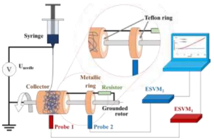
Fig. 1 presents the sketch of the experimental setup of electrospinning. The polymer solutions were fed by a syringe pump (Fischer scientific) at 1 mL/h with a stainless steel needle having an inner diameter of 0.5 mm. The needle was electrically connected to a DC power supply (Spellman SL10). The needle-to-collector distance was fixed at 15 cm. The cylindrical collector (diameter = 110 mm and width = 30 mm) was mounted around the rotor connected to the ground, an insulating Teflon ring was fixed between the collector and the rotor to avoid any
charge transfer directly from the collector to the rotor. The collector was electrically connected to a metallic ring at a distance of 20 cm from the collector to avoid any fibers deposition on this ring. The metallic ring was mechanically linked to the rotor by a thick insulating ring of Teflon. A resistor of 500 MΩ was installed between the ring and the rotor connected to the ground allowing the calculation of the electrospinning current from the measurement of the potential of the metallic ring, thanks to the Ohm’s law. The velocity of rotation of the rotor was set at 120 rpm.
To measure the surface potential at the top surface of the membrane, a non-contacting electrostatic voltmeter ESVM1 (Trek Model 347-3-H-CE) connected to a computer for data
acquisition was used. The measurement is based on a field-nulling technique for non-contacting voltage measurement achieving direct current stability and high accuracy, with no need for fixed probe-to-surface spacing. The technique allows an accurate measurement of the surface potential of stationary or moving surfaces. The measurement range is 0 to ± 3 kV with an accuracy of 0.1% of the full range. The probe (Probe 1) of the voltmeter (probe model 6000B-7C with a speed of response of 4.5 ms for 1 kV step) having a disc surface of 11.2 mm diameter was placed 2 mm below the surface of the collector as shown in Fig 1. An acquisition rate of 30 measurements/s was chosen.
To measure the potential at the bottom of the membrane connected to the metallic ring, a non-contacting electrostatic voltmeter ESVM2 (Trek Model 323-H-CE) connected to a computer for
data acquisition was used. The measurement range is 0 to ± 100 V with an accuracy of 0.05% of the full range. The probe (Probe 2) of the voltmeter (probe model 6000B-16 with a speed of response of 300 ms for 100 V step) having a square surface of 9.5×9.5 mm2 was placed 2 mm below the surface of the supplementary ring as shown in Fig 1. An acquisition rate of 30 measurements/s was chosen.
2.3 SEM measurements
The morphology of fibers and particles was studied by scanning electron microscopy (SEM) (Vega-3, Tescan). The samples were gold coated (sputter Quorum Q 150 RS, Quorum Technologies) for 2 min before SEM characterization. Fiber diameters are given in Table 1.
3. Results
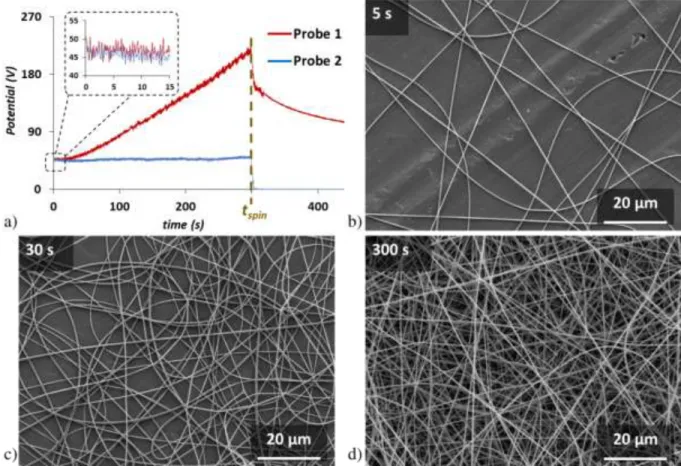
Fig. 2a shows the potential at the bottom of the fibers mat and the surface potential 𝑉 over the membrane recorded during 𝑡𝑠𝑝𝑖𝑛= 300 s of electrospinning PLA in the case of PLA-S2 conditions (see Table 1) and after stopping electrospinning (for 𝑡 > 𝑡𝑠𝑝𝑖𝑛). The measurement of
the potential of the collector (Probe 2, see Fig. 1 and 2a), i.e. the potential below the membrane, corresponds to the difference of potential through the resistor 𝑅 and allows the calculation of the current 𝑖, induced by the flow of charges through the membrane, thanks to the Ohm’s law. The current 𝑖 is constant during the time of electrospinning demonstrating that the electrospun jet brings a constant amount of charges per unit time. However, the surface potential (Probe 1, see Fig. 1 and 2a) increases along the time of production due to residual charges accumulating in the membrane. During the first time of electrospinning, t ≤ 15 s, the surface potential is almost constant. Indeed, as observed in Fig. 2b in the case of fibers deposited after a short time 𝑡𝑠𝑝𝑖𝑛 = 5 𝑠 , the fibers are in good contact with the collector favoring an efficient charge
dissipation which results in poor charge accumulation and thus only a slight increase of the surface potential. For a larger time 𝑡𝑠𝑝𝑖𝑛 = 30 𝑠, Fig. 2c shows that the direct electric contact with the collector is lost between the incoming jet and the layer of fibers deposited in the very first time. The suspended fiber strands cannot release their charges anymore: the surface potential starts to increase significantly. Then, a steady state behavior is reached during which
the surface potential increases significantly and linearly as a function of time. The slope 𝑑𝑉/𝑑𝑡 is thus constant during this period and the fibrous and porous morphology of the produced membrane is stable. When electrospinning is stopped at 𝑡𝑠𝑝𝑖𝑛, the current is no longer brought
by the electrospun jet leading immediately to the return at 0V of the collector's potential. During the same time, after having instantaneously decreased of a value of 𝑅𝑖, the surface potential over the membrane continues to decrease slowly due to the release of the charges stored during electrospinning. In order to get more insight into these experimental results, a model allowing the prediction of the evolution of the surface potential of the membrane during electrospinning is proposed.
Fig. 1. Sketch of the experimental setup allowing the measurement of the membrane surface potential (Probe 1) and the potential at the bottom of the membrane (Probe 2).
Fig. 2. Electrospinning in the case of PLA-S2 conditions. a) Evolution of the surface potential over the membrane (Probe 1) and on the collector (i.e. at the membrane-collector interface, Probe 2) during tspin = 300 𝑠 of electrospinning and after stopping electrospinning at tspin.
SEM pictures obtained after b) tspin = 5 𝑠, c) tspin = 30 𝑠 and tspin = 300 𝑠 under PLA-S2 conditions.
3.1 In-situ charging under different parameters during electrospinning Evolution of the membrane surface potential during electrospinning: a model
Electrospinning can be seen as a process allowing the layer by layer building of a porous membrane. The electric behavior is depicted in Fig. 3. At time 𝑡, when the jet, having a linear charge density λ, enters in contact with the top surface of the membrane, it starts to release its charges towards the ground along the electrical circuit formed by the interconnected fibers. At the same time, the freshly deposited fiber starts to build the layer of pores located at the top
surface of the membrane. The elementary domain of this interconnected circuit is the pore which is a small volume of air surrounded by charged fiber segments. Consequently, one pore may be modeled by a parallel resistor-capacitor circuit (Fig. 3) having a characteristic time 𝜏 = 𝑅𝑝𝐶𝑝. The capacitance 𝐶𝑝 may be linked with the pore size, the capacitor being made of a dielectric, the air, surrounded by the charged electrodes, the fiber strands. The resistance 𝑅𝑝 of
the elementary circuit may be linked with the intrinsic resistivity of the fiber, the quality of the fiber-fiber contact points and the number of contact points per unit volume of membrane. During the deposition process, the electrospun jet brings a constant amount of charges per unit time, thus the elementary current 𝑖𝑝 flowing through the 𝑅𝑝𝐶𝑝 circuit is constant during time 𝑡.
Fig. 3. Charge accumulation during electrospinning. The fibers form an interconnected electrical circuit and the pore can be modeled by a resistor-capacitor 𝑅𝑝𝐶𝑝 circuit.
If the 𝑅𝑝𝐶𝑝 circuit is formed at time 𝑡′, it is thus subjected to the following difference of potential 𝑑𝑢(𝑡):
𝑑𝑢(𝑡)= (1 − 𝑒−(𝑡−𝑡
′) 𝜏⁄
)𝑖𝑝𝑅𝑝 (1)
Assuming that the membrane has an electrical resistance 𝑅𝑚 and a surface 𝑆𝑚, an
average of 𝑃 = 𝑆𝑚⁄𝐷𝑝2 pores of diameter 𝐷
𝑝 forms an elementary porous layer of membrane
made of 𝑃 𝑅𝑝𝐶𝑝 circuits in parallel (depicted in red in Fig. 3). The equivalent resistance of such
Consequently, the elementary layer of pores has the same difference of potential 𝑑𝑢(𝑡) as a single pore as well as the same characteristic time 𝜏 = 𝑑𝑅𝑚𝑑𝐶𝑚 = 𝑅𝑝𝐶𝑝. Furthermore, the current flowing through the elementary layer of pores corresponds to the total electrospinning current i. Thus, a porous layer of thickness 𝑑𝑦 at position 𝑦 and formed at time 𝑡′, is subjected
to the following difference of potential at time 𝑡:
𝑑𝑢(𝑡)= (1 − 𝑒−(𝑡−𝑡
′) 𝜏⁄
)𝑖𝑑𝑅𝑚 (2)
The surface potential at time 𝑡 of the membrane having a thickness ℎ(𝑡) is the sum of the potential 𝑑𝑢(𝑡) of all elementary layers plus the difference of potential through the resistor 𝑅 used for the measurement of the current:
𝑉(𝑡) = 𝑅𝑖 + ∫ 𝑑𝑢(𝑡) ℎ(𝑡) 0 = 𝑅𝑖 + ∫ (1 − 𝑒 −(𝑡−𝑡′) 𝜏⁄ )𝑖𝑑𝑅𝑚 𝑑𝑡′ 𝑑𝑡 ′ 𝑡 0 (3)
It is assumed that the rate of resistance 𝑅̇𝑚 =𝑑𝑅𝑚
𝑑𝑡′ and the characteristic time 𝜏 are constant. Thus, after integration of equation (3), the surface potential can be expressed as:
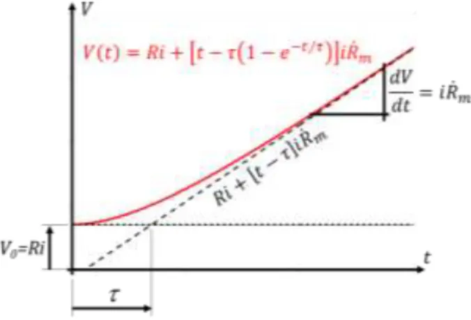
𝑉(𝑡) = 𝑅𝑖 + [𝑡 − 𝜏(1 − 𝑒−𝑡 𝜏⁄ )]𝑖𝑅̇𝑚 (4)
Fig. 4 shows the trend of 𝑉 as a function of 𝑡 and how the parameters 𝑖, 𝜏 and 𝑅̇𝑚 can be
graphically obtained. It is seen that:
𝑉(𝑡 ≪ 𝜏) ~ 𝑉(𝑦 = 0) = 𝑉0 = 𝑅𝑖 (5)
𝑉0 corresponds to the potential at the collector-membrane interface (i.e. at the position y = 0)
and can be easily measured in order to get the current 𝑖.
When 𝑡 ≪ 𝜏, the surface potential is almost constant. Indeed, the characteristic time is the time it takes to completely charge a layer of characteristic thickness ℎ𝜏. When 𝑡 ≫ 𝜏, all the layers located below the upper layer of fibers of characteristic thickness ℎ𝜏 are completely charged and are equivalent to a resistive layer of interconnected fibers having a thickness of ℎ(𝑡) − ℎ𝜏.
Under this condition, the surface potential evolves linearly with time:
Fig. 4. Theoretical evolution of the membrane surface potential as a function of the time and the characteristic parameters 𝑉0, 𝑖, 𝜏 and 𝑅̇𝑚 of the curve.
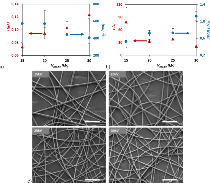
Effect of applied voltage during electrospinning
Experimental curves of the surface potential as a function of time for various applied voltages are given in Fig. S1b of Supp. Data. Fig. 5a shows that the current, corresponding to the amount of charges brought by the jet per unit time, increases obviously with the applied voltage. The final slope of the surface potential, corresponding to 𝑑𝑉
𝑑𝑡 = 𝑖𝑅̇𝑚, is almost constant
from 15 kV to 25 kV (Fig. 5b). An increase of 𝑖𝑅̇𝑚 is observed for the highest voltage, i.e. at 30 kV, meaning that for this condition the resistance of the membrane increases faster than in the other cases. It was observed by SEM that when the voltage increases continuously, a more intense electrostatic force acts on the jet resulting in thinner fibers and more efficient solvent evaporation (see Table 1 and Fig. S1a of Supp. data). Indeed, for the lowest applied voltage, fusion among fibers at their contact points is observed resulting in an overall lower membrane electrical resistance. From Fig. 5b, it is also shown that the characteristic time 𝜏 decreases gradually with the increase of the voltage, with a value changing from 79s to 21s when increasing the applied voltage at the emitter from 15kV to 30kV. Furthermore, it is shown that the fiber diameter decreases with the applied voltage (Fig. 5a and 5c) resulting thus to a
decrease of the average pore size of the fibrous mesh.[31] As shown in the previous section, the characteristic time relies on the average pore size having each a capacitance directly correlated with their size. Thus, a decrease in the fiber diameter results in the production of membranes with smaller pores and consequently a decrease of the capacitance 𝐶𝑝 and the characteristic time 𝜏.
a) b)
c)
Fig. 5. a) Evolution of the current (red triangles) and the fiber diameter (blue discus) as a function of the applied voltage. b) Characteristic time 𝜏 (red triangles) and slope 𝑑𝑉
𝑑𝑡 = 𝑖𝑅̇𝑚
(blue discus) as a function of the applied voltage. c) SEM pictures of PLA fibers prepared at different applied voltages (PLA-S5, S6, S2 and S7 conditions, scale bar = 10 µm).
200 400 600 800 0,06 0,08 0,10 0,12 0,14 15 20 25 30 ϕf ( n m ) i ( µ A ) Vneedle (kV) 0,2 0,6 1,0 1,4 0 30 60 90 120 15 20 25 30 d V /d t (V /s ) τ (s ) Vneedle (kV)
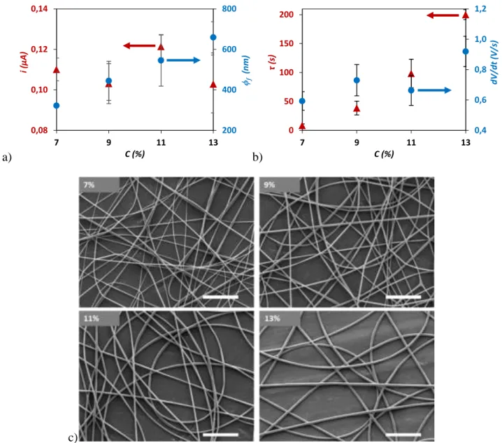
Effect of Polymer concentration during electrospinning
As shown in Fig. 6a, the polymer concentration in the solution does not impact significantly the current, the values varying from 0.09 µA to 0.13 µA when changing the concentration from 7% to 13%. Actually, the current is the consequence of complex mechanisms. Indeed, regarding the polymer alone, at constant solution feeding rate (i.e. 1 mL/h), an increase of the polymer concentration results in the increase of the fiber flow rate increasing thus the rate of charges landing on the collector and consequently the current. Concurrently, increasing the concentration induces the enlargement of the solution viscosity decreasing thus the efficient production of fiber and consequently, the current. In our case, these two phenomena being in competition resulted in a current which is almost constant with the concentration. However, as shown in Fig. 6b and Fig. S2b of Supp. Data, τ increases gradually and significantly from 8 s to 200 s when the concentration increases from 7% to 13% whereas the slope 𝑖𝑅̇𝑚 is almost
constant with, however, a small increase observed for the highest studied concentration. Once again, the characteristic time seems to be in good correlation with the size of the pores being proportional with the fiber diameter (Fig. 6c). Thus, as shown in Fig. 6a, increasing the polymer concentration induces the enlargement of the fiber diameter due to high solution viscosities and thus leads to remarkable increase of 𝜏 but with a low effect on the slope 𝑑𝑉
𝑑𝑡 = 𝑖𝑅̇𝑚. It is also
worth noting that for the highest concentration C = 13%, a lag time of 37 s was used to fit adequately the experimental curve of the surface potential. The presence of this lag time could be explained because at high concentration solvent can remain in the fiber when it lands on the collector. This residual solvent could enhance the electrical contact between the first layer of fibers and the collector. Thus, this first fibrous layer could have a very low resistance inducing no rise of the surface potential during this lag time.
a) b)
c)
Fig. 6. a) Evolution of the current (red triangles) and the fiber diameter (blue discus) as a function of the polymer concentration. b) Characteristic time 𝜏 (red triangles) and slope
𝑑𝑉
𝑑𝑡 = 𝑖𝑅̇𝑚 (blue discus) as a function of the polymer concentration in the solution. c) SEM
images of PLA fibers fabricated from polymer solutions at various concentrations (PLA-S1, S2, S3 and S4 conditions, scale bar = 10 µm).
200 400 600 800 0,08 0,10 0,12 0,14 7 9 11 13 ϕf ( n m ) i ( µ A ) C (%) 0,4 0,6 0,8 1,0 1,2 0 50 100 150 200 7 9 11 13 d V /d t (V /s ) τ (s ) C (%)
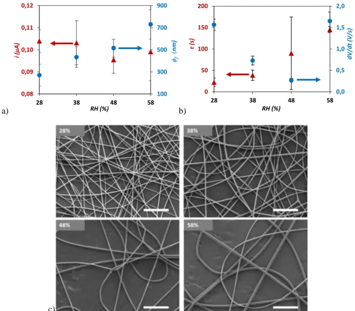
Effect of Ambient relative humidity during electrospinning
No significant effect of the ambient relative humidity (RH) on the current was observed (Fig. 7a). The current being influenced by many parameters, it is complex to draw any conclusion. In contrary, the two main parameters, 𝜏 and 𝑖𝑅̇𝑚, describing the surface potential model evolve significantly with RH (see Fig. 7b and Fig. S3b of Supp. Data). First, a gradual increase of τ was observed. Once more, it can be noticed that 𝜏 increases with the pore size of the membrane. Indeed, as measured by SEM, the fiber diameter increases sharply with RH (Table 1, Fig. 7a and 7c) resulting in the formation of larger pores [31]. It was also observed an effect of RH on the slope 𝑖𝑅̇𝑚 of the curves representing the surface potential as a function of time. A significant decrease of 𝑖𝑅̇𝑚 is firstly observed when RH increases from 28% to 48%. Then, the
slope 𝑑𝑉
𝑑𝑡 = 𝑖𝑅̇𝑚 is rising sharply when increasing RH from 48% to 58%. These results show that
RH mainly affects the electrical resistance rate of the membrane 𝑅̇𝑚 instead of 𝑖𝑅̇𝑚, the current being indeed almost constant with RH . The membrane resistance 𝑅𝑚 is linked with the resistivity of the polymer, here PLA, the quality of the fiber-fiber contact points and the number of contact points per unit volume of membrane. As shown in Fig. S3a of Supp. Data, all these features seem to change as a function of RH explaining thus the complex trend of 𝑖𝑅̇𝑚.
a) b)
c)
Fig. 7. a) Evolution of the current (red triangles) and the fiber diameter (blue discus) as a function of the relative humidity. b) Characteristic time 𝜏 (red triangles) and slope 𝑑𝑉
𝑑𝑡 = 𝑖𝑅̇𝑚
(blue discus) as a function of the relative humidity. c) SEM images of PLA fibers fabricated from various ambient relative humidity (PLA-S8, S2, S9 and S10 conditions, scale bar = 10
µm). 100 300 500 700 900 0,08 0,09 0,10 0,11 0,12 28 38 48 58 ϕf (n m ) i ( µ A ) RH (%) 0,0 0,5 1,0 1,5 2,0 0 50 100 150 200 28 38 48 58 d V /d t (V /s ) τ (s ) RH (%)
3.2 Decay of the surface potential of the membrane after stopping the fiber production – mechanism of residual charges dissipation
Surface potential decay: a model
In this section, the stored charges release mechanism is studied over after stopping electrospinning. When the power supply connected to the emitter is switched-off, the jet is no more produced, the current is thus equal to zero and no more charges are deposited. Since the current is null, no charges are released to the ground. However, a decrease of the surface potential over time is observed as shown in Fig. 8. Several mechanisms of charge release can explain the surface potential decay. First, charges located at the topmost surface of the membrane are subjected to ion neutralization with air. This charge release phenomenon may occur at short times, characterized by a time denoted 𝜏𝑠. Second, charges mostly located at the
surface of the fibers, but inside the porosity of the membrane, should release their charges within each pore having already participated to the kinetic of in-situ charging by electrospinning. It is thus expected that this second characteristic time of decay, denoted 𝜏𝑚, is in the same order than the characteristic time τ measured during in-situ charging. This medium characteristic time 𝜏𝑚 is expected to be higher than 𝜏𝑠. Third, in-situ electrospinning may lead the production of charges efficiently trapped in the bulk of the fibers. Indeed, although electrospinning of PLA leads to the fabrication of fibers with low crystallinity [29], charges may be trapped inside the fibers between amorphous and crystalline domains. This charge release phenomenon may occur at long times characterized by a time denoted 𝜏𝑙. Thus,
although a double exponential fitting was proposed in the literature for fibrous membranes charged by corona effect[32], it is expected that the surface potential decay may be modeled by the sum of three exponential functions as follows:
𝑉(𝑡) = 𝐴𝑠𝑒 −(𝑡−𝑡𝑠𝑝𝑖𝑛 𝜏𝑠 )+ 𝐴𝑚𝑒−( 𝑡−𝑡𝑠𝑝𝑖𝑛 𝜏𝑚 )+ 𝐴𝑙𝑒−( 𝑡−𝑡𝑠𝑝𝑖𝑛 𝜏𝑙 ) (7)
Fig. 8. Surface potential decay after stopping electrospinning carried out under the conditions of PLA-S2 (see Table 1). Experimental data (grey line), model with two characteristic times
only (short dashed blue line), model with 2 characteristic times and one asymptote (dashed green line), model with three characteristic times only (dashed-point red line).
Fig. 8 shows the surface potential decay obtained after stopping electrospinning carried out under the conditions of PLA-S2 with a long time of acquisition of 2000 s. The model described by Eqn. 7 fits perfectly the experimental data. After fitting by a least square method, the obtained times were respectively 𝜏𝑠=11 s, 𝜏𝑚 =104 s and 𝜏𝑙 =2183 s. A double exponential model was tested in order to compare the fitting quality:
𝑉(𝑡) = 𝐴1𝑒
−(𝑡−𝑡𝑠𝑝𝑖𝑛
𝜏1 )+ 𝐴2𝑒−(
𝑡−𝑡𝑠𝑝𝑖𝑛
𝜏2 ) (8)
Using Eqn. 8, one characteristic time is obviously lost, leading to bad fitting as shown in Fig. 8. In this case, the obtained characteristic times were 𝜏1=51 s and 𝜏2 =1187 s. Another model
can be proposed, using also two characteristic times but introducing an asymptote 𝑉∞ instead of the long time as introduced in the model described by Eqn. 7. The model is the following:
𝑉(𝑡) = 𝑉∞+ 𝐴𝑠𝑒
−(𝑡−𝑡𝑠𝑝𝑖𝑛
𝜏𝑠 )+ 𝐴𝑚𝑒−(
𝑡−𝑡𝑠𝑝𝑖𝑛
𝜏𝑚 ) (9)
Eqn. 9 also allows a good fitting of the experimental data as 𝑉∞ can also be linked to the behavior at long times whereas 𝜏𝑠 and 𝜏𝑚 play the same role as in the model using three
characteristic times. Using Eqn. 9, the least square method gave the corresponding characteristic times: 𝜏𝑠 =17 s and 𝜏𝑚 =166 s. Because in the next part, all measurements of the surface potential decay were carried out during a time of 150 s, the three exponential model didn’t allow a good estimation of the long time 𝜏𝑙. Thus, the model using two characteristic
times with an asymptote 𝑉∞ (Eqn. 9) was chosen to fit the experimental data and only the behavior at short and medium times was studied. Furthermore, the following normalized weight factors were also studied as a function of the processing conditions:
𝐴𝑠% = 100 𝐴𝑠 𝑉∞+𝐴𝑠+𝐴𝑚 (10) 𝐴𝑚% = 100 𝐴𝑚 𝑉∞+𝐴𝑠+𝐴𝑚 (11) 𝑉∞% = 100 𝑉∞ 𝑉∞+𝐴𝑠+𝐴𝑚 (12)
Effect of Applied voltage on the surface potential decay after stopping electrospinning
Fig. 9 presents both 𝜏𝑠 and 𝜏𝑚 obtained from Eqn. 9 to fit the surface potential decay measured after applying various voltages on the emitter. The curves giving the surface potential decay as a function of time for various applied voltage are given in Fig. S4 of Supp. Data. It should be mentioned that the two exponentials are needed to fit adequately all experimental data. The normalized weight factors are not influenced by the applied voltage whereas the medium decay process is preponderant compared to the short one. The discharged of the top surface, characterized by the short time 𝜏𝑠 being in the order of 10 s, is a little bit faster for the membranes produced for the highest voltage. Indeed, the highest applied voltage led to the
production of membranes with the thinnest fibers and consequently having the largest surface area offered to the ions of the air for a quick decay. It is also shown that the short time decay is around ten times faster than the medium one. A slow decrease of the medium time with applied voltage is observed. Moreover, 𝜏𝑚 is of the same order of magnitude than the characteristic time 𝜏 determined from the modeling of the surface potential during in-situ charging by electrospinning. These features seem to show that 𝜏𝑚 and 𝜏 rely on the same physical mechanisms originating from the effect of the pores of the membrane on the kinetic of the surface potential. However, the effect of applied voltage on 𝜏𝑚 is weaker than what was observed for τ during electrospinning. Although efficient charge injection is expected in the bulk of the fibers produced for the highest applied voltage, it is observed that 𝑉∞% , characterizing the amount of bulk charges, is surprisingly constant with applied voltage. However, such result must be taken with caution because the measurements were carried out along short period, i.e.150 s, that don’t allow a precise description of the kinetic at long times.
a) b)
Fig. 9. a) Short 𝜏𝑠 (blue discus) and medium 𝜏𝑚 (red triangles) times and b) normalized weight factors (𝐴𝑠: blue discus, 𝐴𝑚: red triangles, 𝑉∞: green squares) as a function of applied voltage
on the emitter. 60 90 120 0 5 10 15 20 15 20 25 30 τm ( s) τs ( s) Vneedle (kV) 0 20 40 60 15 20 25 30 No rm a lize d we ig h t fa cto r (% ) Vneedle (kV)
Effect of Polymer concentration on the surface potential decay
Fig. 10 shows 𝜏𝑠 and 𝜏𝑚 in the case of membranes produced at various polymer concentrations. The curves giving the surface potential decay as a function of time for various polymer concentrations are shown in Fig. S5 of Supp. Data. The normalized weight factors are not significantly influenced by the polymer concentration. As observed for 𝜏 during in-situ charging, 𝜏𝑚 increases with the polymer concentration. However, the trend of 𝜏𝑚 is much less pronounced than for 𝜏. No tendency can be draw for the short time decay.
a) b)
Fig. 10. a) Short 𝜏𝑠 (blue discus) and medium 𝜏𝑚 (red triangles) times and b) normalized
weight factors (𝐴𝑠: blue discus, 𝐴𝑚: red triangles, 𝑉∞: green squares) as a function of polymer concentration.
Effect of Ambient relative humidity on the surface potential decay
Fig. 11 shows 𝜏𝑠 and 𝜏𝑚 obtained to fit the surface potential decay measured for various ambient relative humidity (RH). The curves giving the surface potential decay as a function of time for various RH are shown in Fig. S6 of Supp. Data. Compared with the effect of the two previous parameters (applied voltage and polymer concentration) on the characteristic times, the effect of RH is more pronounced. This should be explained by the fact that RH is imposed not only during in-situ charging by electrospinning but also after stopping electrospinning. As
60 70 80 90 100 0 2 4 6 8 10 12 14 7 9 11 13 τm (s ) τs ( s) C (%) 0 20 40 60 80 7 9 11 13 No rm a lize d we ig h t fa cto r (% ) C (%)
observed for 𝜏 , 𝜏𝑚 increases with RH , 𝜏𝑚 being in the same order of magnitude than 𝜏 .
Furthermore, it is worth noting that the fact that RH influences almost only the charges located on the surface of the fibers confirms that the mechanism leading to the surface potential decay at medium time 𝜏𝑚 is due to the release of surface charges and not to bulk charges inside the
fibers. Finally, a significant increase of 𝑉∞% is observed for the highest RH showing that a high
amount of bulk charges, having the longest characteristic times, are stored in the matrix of the fibers. Indeed, because PLA is a hydrophobic polymer, diffusion of water into the electrospun jet results in the rapid precipitation of PLA [33]. Such rapid precipitation may lead to a high amount of defects in the polymer matrix explaining thus the high amount of charges which are usually trapped in the defects [16].
a) b)
Fig. 11. a) Short 𝜏𝑠 (blue discus) and medium 𝜏𝑚 (red triangles) times and b) normalized
weight factors (𝐴𝑠: blue discus, 𝐴𝑚: red triangles, 𝑉∞: green squares) as a function of relative humidity
4. Discussion
Although the measurement of the surface potential decay allows to finally dissociating the kinetic in three fundamental mechanisms of charge release, it only gives an average behavior over the entire thickness of the membrane. In contrary, the measurement of the surface potential during in-situ charging by electrospinning is mainly sensitive to the kinetic of charge release at
40 60 80 100 120 140 0 2 4 6 8 10 12 14 28 38 48 58 τm ( s) τs ( s) RH (%) 0 30 60 90 28 38 48 58 No rm a lize d we ig h t fa cto r (% ) RH (%)
medium times but with a much higher accuracy. Indeed, the medium time 𝜏𝑚, obtained from
the fitting of the surface potential decay measured after stopping electrospinning, is of the same order of magnitude than the time 𝜏 measured during electrospinning. Both 𝜏𝑚 and 𝜏 follow the same behavior as a function of the studied processing parameters: a decrease with increasing voltage and the opposite when increasing either the polymer concentration or the ambient relative humidity. However, the characteristic time 𝜏 revealed to be much more sensitive than 𝜏𝑚. Such difference can be explained by the fact that the surface potential measured during
electrospinning takes into account a continuously fresh deposited top surface which immediately starts to release its charges. Thus, 𝜏 may be more related to the combination of the release at short times ( 10 s) of charges located on the top surface and the release at medium times ( 100 s) of the charges located in the pores just below the top surface under construction. In fact, in the proposed model of in-situ charging by electrospinning (Eqn. 4), the 𝜏 value can be related to the electrical characteristics at the different length scales: (i) the pore, (ii) the elementary layer having the surface of the membrane and the thickness of one pore and (iii) the whole membrane under building. Each of them is related to the pore structure of the membrane:
𝜏 = 𝑑𝑅𝑚𝑑𝐶𝑚 = 𝑅𝑝𝐶𝑝= 𝑅𝑚𝐶𝑚 (13)
Assuming that the membrane electrical resistance 𝑅𝑚 evolves linearly with time:
𝑅𝑚 = 𝑅̇𝑚𝑡 (14)
And using equations 13 and 14, it is possible to give an estimation of the membrane capacitance 𝐶𝑚:
𝐶𝑚= 𝜏
𝑅̇𝑚𝑡 (15)
Because the number of elementary layers in the thickness of the membrane is proportional to the time of deposition and that the current is constant during time, 𝑑𝑅𝑚 and 𝑑𝐶𝑚 scale as:
𝑑𝐶𝑚 ∝ 𝜏 𝑅̇𝑚∝
𝜏
𝑑𝑉/𝑑𝑡 (17)
Thus, knowing that the average number of pores 𝑃 for one elementary layer of membrane of surface 𝑆𝑚 is 𝑃 = 𝑆𝑚⁄𝐷𝑝2 and that the characteristic size of a pore 𝐷
𝑝 is proportional to the
fiber diameter 𝐷𝑝~𝜙𝑓,[31] the resistance and the capacitance of a pore scale respectively as:
𝑅𝑝 ∝ 𝑑𝑉/𝑑𝑡 𝜙𝑓2 (18) 𝐶𝑝 ∝ 𝜙𝑓2 𝜏 𝑑𝑉/𝑑𝑡 (19) a) b)
Fig. 12. a) Correlation between 𝐶𝑝 and the fiber diameter 𝜙𝑓. b) Correlation between the fiber
diameter 𝜙𝑓 and 𝜏 (𝑑𝑉/𝑑𝑡)⁄ . Green triangles correspond to the experimental points obtained from polymer concentrations C = 7 %, 9 %, 11 % and 13 %, blue squares from relative humidity RH = 28 %, 38 %, 48 % and 58 % and red discus from applied voltages = 15 kV, 20
kV, 25 kV and 30 kV.
In order to verify the proposed scaling law, all data points obtained in the various operating conditions (applied voltage, polymer concentration and ambient relative humidity) were represented in graphs. The first one, gives 𝜙𝑓
2 𝜏
𝑑𝑉/𝑑𝑡 as a function of the measured fiber diameter 𝜙𝑓
(Fig. 12a). Because of Eqn. 19, this graph is proportional to the graph of the pore capacitance 𝐶𝑝 versus 𝜙𝑓. It is shown that whatever the processing condition (highlighted by the different
symbols in the graph), 𝐶𝑝 is well correlated with the fiber diameter (Fig. 12a). The following scaling law can thus be obtained for electrospinning of PLA on a flat collector:
𝐶𝑝 ∝ 𝜙𝑓4.87 (20)
Consequently, the fiber diameter can also be plotted as a function of 𝜏
𝑑𝑉/𝑑𝑡 and a good
correlation is obtained (Fig. 12b) giving thus 𝜙𝑓 as a function of only the physical quantities
obtained from the measurement of the surface potential:
𝜙𝑓 ∝ [ 𝜏 𝑑𝑉/𝑑𝑡]
0.21
(21)
It is thus shown for the first time that the measurement of the surface potential, thanks to the use of an electrostatic voltmeter, is a simple method giving accurate information at the local scale of the nanofiber diameter of an electrospun membrane. Moreover, such a method should allow the detection of variations in the porous morphology and/or membrane’s quality during its fabrication. In order to illustrate such feature, 0.5wt% of TEBAC salt was added in the PLA solution and electrospun under the conditions PLAsalt-S2 (see Table 1) which are equivalent to the PLA-S2 standard conditions without salt. The addition of the salt brings a high amount of charges in the electrospun jet which explains the significant increase of the current (0.74 µA for PLAsalt-S2 calculated from 𝑉 at 𝑡 = 0 𝑠 compared to 0.1 µA for PLA-S2). Moreover, as opposed to the pure PLA system (see Fig. 2a), the addition of TEBAC perturbs significantly the evolution of the surface potential 𝑉. Indeed, Fig. 13a shows that the surface potential does not increase linearly with time as it was observed in the case of PLA-S2 as well as for all other studied pure PLA systems. The accumulation rate of charges in the membrane, characterized by the slope 𝑑𝑉/𝑑𝑡, is thus not constant during electrospinning. Fig. 13b shows indeed that the salt is not homogeneously distributed which could explain that the charges are not regularly brought by the jet explaining the observed instabilities. The on-line measurement of the surface
potential seems to be an efficient way for the monitoring of the electrospinning stability and quality of the produced membrane.
a) b)
Fig. 13. Effect of the addition of a salt in the solution on the stability of the surface potential obtained during electrospinning with conditions PLAsalt-S2 (see Table 1). a) Evolution of the surface potential. b) SEM picture of PLA fibers with TEBAC salt. The two rings highlight fiber
domains having no salt particles on their surface.
5. Conclusion
Here, we showed that the measurement of the surface potential of the membrane can be easily carried out online during the process of electrospinning using an electrostatic voltmeter. A model was proposed to follow the kinetics of the surface potential during in-situ charging by electrospinning for various operating conditions. The model is characterized by a characteristic time 𝜏, linked to the formation of an elementary porous layer of the membrane and by the slope
𝑑𝑉/𝑑𝑡, measured at steady state, and related to the electrical resistance of the membrane induced by the fiber resistivity and the quality and the density of fiber-fiber contact points. The kinetic of the surface potential decay after stopping electrospinning was also studied. Three characteristic times can be identified during scaffold discharge. A short time 𝜏𝑠, having a value in the range of ten seconds, can be correlated to the rapid charge release occurring on the
topmost surface of the membrane. A medium time 𝜏𝑚, having a value of several tens of seconds
up to more than one hundred of seconds, relies on the charge release inside each pore of the membrane. The times 𝜏𝑚 and 𝜏, having the same physical origin, they are in the same order of magnitude. However, 𝜏 obtained from in-situ charging during electrospinning, is more sensitive to the processing conditions. Finally, the long time 𝜏𝑙, being at least one order of magnitude
higher than the medium time, characterizes the release of the charges trapped in the bulk of the fibers.
The measurement of the surface potential allows thus the detection of variations in the porous morphology of the membrane during its fabrication. Furthermore, in combination with the measurement of the current, it is an efficient and complementary method to get more insight into the overall process of electrospinning for a robust online monitoring. Last but not least, the method also gives immediate information on the residual charges stored in the fibrous membrane which is an important feature for the elaboration, by electrospinning in-situ charging, of electrets for filtering applications.
Supplementary Data. Curves of surface potential and complementary SEM pictures related to this article can be found online free of charge at https://doi.org/10.1016/j.polymer.XXXXXXXXXXXXX Acknowledgements
The authors are grateful to the French National Research Agency for the financial support of this work (Project MimHeart ANR-15-CE08-0010-02). We thank China Scholarship Council (CSC) for the financial support of the PhD student. We also thank Christophe Sutter, Christophe Mélart, Michel Wolf and Thierry Djekriff for their help in the electrospinning set up.
References
[1] S. Wang, X. Zhao, X. Yin, J. Yu, B. Ding, Electret Polyvinylidene Fluoride Nanofibers Hybridized by Polytetrafluoroethylene Nanoparticles for High-Efficiency Air Filtration, ACS Applied Materials & Interfaces. 8 (2016) 23985–23994. https://doi.org/10.1021/acsami.6b08262. [2] S. Nedjari, A. Hébraud, S. Eap, S. Siegwald, C. Mélart, N. Benkirane-Jessel, G. Schlatter,
Electrostatic template-assisted deposition of microparticles on electrospun nanofibers: towards microstructured functional biochips for screening applications, RSC Advances. 5 (2015) 83600– 83607. https://doi.org/10.1039/C5RA15931H.
[3] J.-H. Jang, O. Castano, H.-W. Kim, Electrospun materials as potential platforms for bone tissue engineering, Advanced Drug Delivery Reviews. 61 (2009) 1065–1083. https://doi.org/10.1016/j.addr.2009.07.008.
[4] S.Y. Chew, J. Wen, E.K.F. Yim, K.W. Leong, Sustained Release of Proteins from Electrospun
Biodegradable Fibers, Biomacromolecules. 6 (2005) 2017–2024.
https://doi.org/10.1021/bm0501149.
[5] A. Thorvaldsson, H. Stenhamre, P. Gatenholm, P. Walkenström, Electrospinning of Highly Porous Scaffolds for Cartilage Regeneration, Biomacromolecules. 9 (2008) 1044–1049. https://doi.org/10.1021/bm701225a.
[6] J. Xue, T. Wu, Y. Dai, Y. Xia, Electrospinning and Electrospun Nanofibers: Methods, Materials,
and Applications, Chemical Reviews. 119 (2019) 5298–5415.
https://doi.org/10.1021/acs.chemrev.8b00593.
[7] M. Zhu, J. Han, F. Wang, W. Shao, R. Xiong, Q. Zhang, H. Pan, Y. Yang, S.K. Samal, F. Zhang, C. Huang, Electrospun Nanofibers Membranes for Effective Air Filtration, Macromolecular Materials and Engineering. 302 (2017) 1600353. https://doi.org/10.1002/mame.201600353. [8] T. Jiang, E.J. Carbone, K.W.-H. Lo, C.T. Laurencin, Electrospinning of polymer nanofibers for
tissue regeneration, Progress in Polymer Science. 46 (2015) 1–24. https://doi.org/10.1016/j.progpolymsci.2014.12.001.
[9] R. Samatham, K.J. Kim, Electric current as a control variable in the electrospinning process, Polymer Engineering & Science. 46 (2006) 954–959. https://doi.org/10.1002/pen.20565.
[10] F. Yener, B. Yalcinkaya, O. Jirsak, On the Measured Current in Needle- and Needleless Electrospinning, Journal of Nanoscience and Nanotechnology. 13 (2013) 4672–4679. https://doi.org/10.1166/jnn.2013.7189.
[11] Y.M. Shin, M.M. Hohman, M.P. Brenner, G.C. Rutledge, Experimental characterization of electrospinning: the electrically forced jet and instabilities, Polymer. 42 (2001) 09955–09967. https://doi.org/10.1016/S0032-3861(01)00540-7.
[12] A.Y. Choi, H.J. Sim, M.K. Shin, S.J. Kim, Y.T. Kim, Residual Charges during Electrospinning Assist in Formation of Piezoelectricity in Poly(Vinylidene Fluoride-co-Trifluoroethylene)
Nanofibers, Journal of Nano Research. 37 (2015) 13–19.
https://doi.org/10.4028/www.scientific.net/JNanoR.37.13.
[13] J. Lowell, Absorption and conduction currents in polymers: a unified model, Journal of Physics D: Applied Physics. 23 (1990) 205–210. https://doi.org/10.1088/0022-3727/23/2/011.
[14] L.H. Catalani, G. Collins, M. Jaffe, Evidence for Molecular Orientation and Residual Charge in the Electrospinning of Poly(butylene terephthalate) Nanofibers, Macromolecules. 40 (2007) 1693–1697. https://doi.org/10.1021/ma061342d.
[15] M. Ignatova, T. Yovcheva, A. Viraneva, G. Mekishev, N. Manolova, I. Rashkov, Study of charge storage in the nanofibrous poly(ethylene terephthalate) electrets prepared by electrospinning or by corona discharge method, European Polymer Journal. 44 (2008) 1962–1967. https://doi.org/10.1016/j.eurpolymj.2008.04.027.
[16] H. Gao, W. He, Y.-B. Zhao, D.M. Opris, G. Xu, J. Wang, Electret mechanisms and kinetics of electrospun nanofiber membranes and lifetime in filtration applications in comparison with corona-charged membranes, Journal of Membrane Science. 600 (2020) 117879. https://doi.org/10.1016/j.memsci.2020.117879.
[17] A. Amin, A.A. Merati, S.H. Bahrami, R. Bagherzadeh, Effects of porosity gradient of multilayered electrospun nanofibre mats on air filtration efficiency, The Journal of The Textile Institute. 108 (2017) 1563–1571. https://doi.org/10.1080/00405000.2016.1264856.
[18] B. Tabti, L. Dascalescu, M. Plopeanu, A. Antoniu, M. Mekideche, Factors that influence the corona charging of fibrous dielectric materials, Journal of Electrostatics. 67 (2009) 193–197. https://doi.org/10.1016/j.elstat.2009.01.047.
[19] B.M. Cho, Y.S. Nam, J.Y. Cheon, W.H. Park, Residual charge and filtration efficiency of polycarbonate fibrous membranes prepared by electrospinning, Journal of Applied Polymer Science. 132 (2015). https://doi.org/10.1002/app.41340.
[20] H.-W. Tong, M. Wang, W.W. Lu, Enhancing the biological performance of osteoconductive nanocomposite scaffolds through negative voltage electrospinning, Nanomedicine. 8 (2013) 577– 589. https://doi.org/10.2217/nnm.13.51.
[21] B. Yalcinkaya, F.C. Callioglu, F. Yener, Measurement and analysis of jet current and jet life in roller electrospinning of polyurethane, Textile Research Journal. 84 (2014) 1720–1728. https://doi.org/10.1177/0040517514528563.
[22] Z. Li, R. Liu, Y. Huang, J. Zhou, Effects of reversed arrangement of electrodes on electrospun nanofibers, Journal of Applied Polymer Science. 134 (2017). https://doi.org/10.1002/app.44687. [23] G. Yan, J. Yu, Y. Qiu, X. Yi, J. Lu, X. Zhou, X. Bai, Self-Assembly of Electrospun Polymer
Nanofibers: A General Phenomenon Generating Honeycomb-Patterned Nanofibrous Structures, Langmuir. 27 (2011) 4285–4289. https://doi.org/10.1021/la1047936.
[24] T. Yao, H. Chen, P. Samal, S. Giselbrecht, M.B. Baker, L. Moroni, Self-assembly of electrospun nanofibers into gradient honeycomb structures, Materials & Design. 168 (2019) 107614. https://doi.org/10.1016/j.matdes.2019.107614.
[25] H.-W. Tong, X. Zhang, M. Wang, A new nanofiber fabrication technique based on coaxial
electrospinning, Materials Letters. 66 (2012) 257–260.
https://doi.org/10.1016/j.matlet.2011.08.095.
[26] S.J. Kim, C.K. Lee, S.I. Kim, Effect of ionic salts on the processing of poly(2-acrylamido-2-methyl-1-propane sulfonic acid) nanofibers, Journal of Applied Polymer Science. 96 (2005) 1388–1393. https://doi.org/10.1002/app.21567.
[27] D. Ahirwal, A. Hébraud, R. Kádár, M. Wilhelm, G. Schlatter, From self-assembly of electrospun nanofibers to 3D cm thick hierarchical foams, Soft Matter. 9 (2013) 3164. https://doi.org/10.1039/c2sm27543k.
[28] N. Lavielle, A.-M. Popa, M. de Geus, A. Hébraud, G. Schlatter, L. Thöny-Meyer, R.M. Rossi, Controlled formation of poly(ε-caprolactone) ultrathin electrospun nanofibers in a hydrolytic degradation-assisted process, European Polymer Journal. 49 (2013) 1331–1336. https://doi.org/10.1016/j.eurpolymj.2013.02.038.
[29] S. Nedjari, S. Eap, A. Hébraud, C.R. Wittmer, N. Benkirane-Jessel, G. Schlatter, Electrospun Honeycomb as Nests for Controlled Osteoblast Spatial Organization, Macromolecular Bioscience. 14 (2014) 1580–1589. https://doi.org/10.1002/mabi.201400226.
[30] S. Nedjari, G. Schlatter, A. Hébraud, Thick electrospun honeycomb scaffolds with controlled pore size, Materials Letters. 142 (2015) 180–183. https://doi.org/10.1016/j.matlet.2014.11.118.
[31] H. Ma, C. Burger, B.S. Hsiao, B. Chu, Ultra-fine cellulose nanofibers: new nano-scale materials for water purification, Journal of Materials Chemistry. 21 (2011) 7507. https://doi.org/10.1039/c0jm04308g.
[32] R. Thakur, D. Das, A. Das, Study of charge decay in corona-charged fibrous electrets, Fibers and Polymers. 15 (2014) 1436–1443. https://doi.org/10.1007/s12221-014-1436-9.
[33] C. Thammawong, S. Buchatip, A. Petchsuk, P. Tangboriboonrat, N. Chanunpanich, M. Opaprakasit, P. Sreearunothai, P. Opaprakasit, Electrospinning of poly(l-lactide-co-dl-lactide) copolymers: Effect of chemical structures and spinning conditions, Polymer Engineering & Science. 54 (2014) 472–480. https://doi.org/10.1002/pen.23576.