HAL Id: hal-01955292
https://hal.archives-ouvertes.fr/hal-01955292
Submitted on 22 Jan 2019
HAL is a multi-disciplinary open access
archive for the deposit and dissemination of
sci-entific research documents, whether they are
pub-lished or not. The documents may come from
teaching and research institutions in France or
abroad, or from public or private research centers.
L’archive ouverte pluridisciplinaire HAL, est
destinée au dépôt et à la diffusion de documents
scientifiques de niveau recherche, publiés ou non,
émanant des établissements d’enseignement et de
recherche français ou étrangers, des laboratoires
publics ou privés.
Dynamic implicit muscles for character skinning
Valentin Roussellet, Nadine Abu Rumman, Florian Canezin, Nicolas Mellado,
Ladislav Kavan, Loic Barthe
To cite this version:
Valentin Roussellet, Nadine Abu Rumman, Florian Canezin, Nicolas Mellado, Ladislav Kavan, et
al.. Dynamic implicit muscles for character skinning. Computers and Graphics, Elsevier, 2018, 77,
pp.227-239. �10.1016/j.cag.2018.10.013�. �hal-01955292�
Dynamic implicit muscles for character skinning
ValentinRoussellet1, NadineAbu Rumman1, FlorianCanezin1
NicolasMellado1, LadislavKavan2, Lo¨ıcBarthe1
1Universit´e de Toulouse, IRIT, CNRS 2University of Utah, School of Computing
Abstract: Most current methods for character skinning can be categorized into 1) geometric techniques, which are fast and easy to use but often lack physical realism, 2) data-driven ap-proaches, which require a large set of examples that are tedious to edit, and 3) physics-based methods, which are highly realistic but slow and difficult to use. Recently introduced geometric Implicit Skinning methods can solve contact interactions and skin elasticity with results comparable to physics-based sim-ulation in real-time. In this paper we introduce an animation method that adds anatomical plausibility while benefiting from the advantages of Implicit Skinning. We propose an efficient way to model muscle primitives with implicit surfaces. Volumetric extrusions of individual muscles are attached to muscle cen-ter lines simulated with a fast, low-dimensional physics-based approach (Position Based Dynamics of one-dimensional line segments). This combination of physics-based simulation with implicit modeling allows us to elegantly resolve muscle-muscle and muscle-bone collisions and add dynamic effects such as flesh jiggling while guaranteeing volume preservation (which is a property of real biological muscles) and producing visually plausible skin-skin contact behavior. Our method runs at inter-active frame-rates and features intuitive modeling parameters which allow animators to quickly explore a variety of designs and physics-based effects.
1. Introduction
Character animation is a central component of animated dig-ital media such as films, computer games, and virtual reality. However, the production of compelling and appealing deforma-tions of a virtual character to imbue it with life remains very challenging due to the complexity of the human (or humanoid) body, which is composed of bones, muscles and soft tissues. Specific challenges include run-time performance and param-eter tuning. Ideally, the resulting deformation models should run interactively on commodity machines and rely only on intu-itive parameters with predictable outcomes on the result. While providing basic skeletal articulation is mandatory to produce animated characters, taking into account the motion of the un-derlying anatomy significantly increases the realism of the final animation. Existing methods simulating the behavior of all anatomic tissues exist, but they require extensive computational resources, limiting their use in interactive applications.
In this paper, we explore the idea of adding muscle defor-mations to skeleton-based geometric skinning approaches. We focus specifically on modelling the muscle’s shape deformation when they contract, expand and activate under effort. Unlike fat
tissues, muscles tend to stay very tense and stiff. We model their elasticity with a dynamic simulation.
Three main families of techniques have been considered to fol-low this direction by extending Linear Blend Skinning (LBS) [1] or Dual Quaternion Skinning (DQS) [2]. The first are pose-based approaches, based on modeling and animation tools, allowing users to edit the character skin in user-specified key poses [3]. Despite being very general and enabling users to model arbitrary skin deformations, manual sculpting is very time-consuming and tedious, especially if similar edits need to be repeated multiple times. A second family of methods uses muscle primitives which are positioned inside the character body and act as deformers generating additional skin deformations, usually designed to preserve volume. Geometric modeling of muscles provides inter-active parameter tuning [4]. However, deformation parameters are often tedious to set and the resulting skinning solution is sub-ject to the well-known Linear Blend Skinning (LBS) and Dual Quaternion Skinning (DQS) limitations, i.e., no skin-contact de-formation and volume loss or gain near joints. The third family is represented by data-driven methods, which learn a set of mesh deformers from captured data [5, 6]. However, the produced deformations are limited by the extent of the training set and the difficulty to artistically control the results.
Our contribution is an approach that combines the advan-tages of muscle primitive deformers with an interactive geo-metric skinning technique producing high-quality skin deforma-tion including contact handling (Figure 1). We rely on Implicit Skinning [7, 8] to resolve self-intersections and represent skin elasticity. However, unlike Implicit Skinning, in this paper we also consider several important phenomena contributing to mus-cle and skin shape, such as musmus-cle-musmus-cle and musmus-cle-bone collisions and dynamic effects induced by the skeletal motion.
Our technical contributions are two-fold: first, we introduce new muscle primitives mimicking the shape and deformation of real muscles (including bulging, deflation, and activation), ranging from relatively simple ones such as the biceps to more complicated pectoral muscles. During animation, our muscles maintain nearly constant volume. We define our muscles as curve-sweep surfaces, with the dynamics of the curves guided by Position Based Dynamics [9]. The use of 3D scalar fields for our muscle primitives enables the integration of these muscles in the Implicit Skinning framework, which provides fast skin-skin contact modeling. The implicit representation of muscles is also perfectly suited for collision response, allowing us to efficiently resolve muscle-bone and muscle-muscle collisions.
Secondly, we show how to adequately integrate our muscle primitives in the Implicit Skinning framework so that the fi-nal skinning solution naturally benefits from its skin contact resolution.
In our implementation, muscle shapes and dynamic behavior are controlled by a small set of intuitive parameters, avoiding the need for tedious sculpting of corrective shapes (as in pose-based methods), as well as expensive computational cost and complicated parameter tuning of physical simulation techniques. During the rigging phase, setting the skinning parameters can be done interactively and the total computation time of our method, given a character including more than fifty animated muscles, is
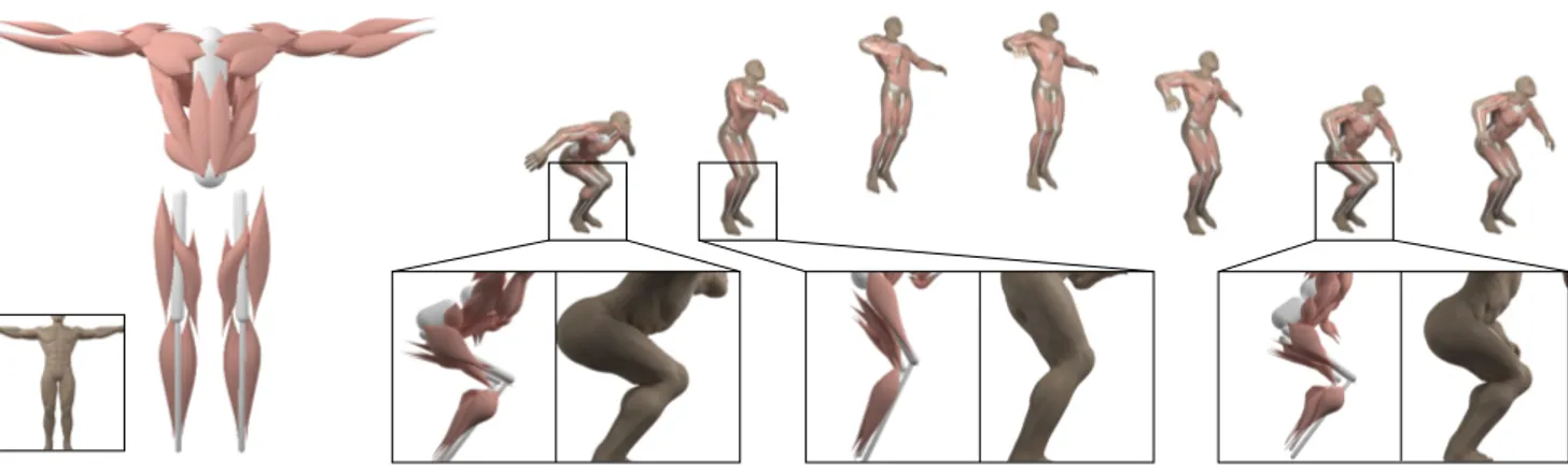
Figure 1. On the left, the muscular and bone structure of the character are shown in the bottom inset. These muscles are represented by new implicit primitives deforming at constant volume with elasticity and collisions computed with Position Based Dynamics. On the right, the different poses of the character jumping illustrate the change in muscle shape due to activation/relaxation, stretch/elongation and the result of the muscle-bone collision resolution. Our muscles adequately seamlessly fit into the Implicit Skinning framework, allowing us to produce character animation with skin contact and elasticity.
less than a second per frame on a standard CPU. 2. Related work
The production of plausible skin-muscle deformations from skeletal motion is a long standing problem in computer anima-tion and several types of approaches emerged in previous work. Capture-based methods. Data-driven methods [10] can be di-vided into 1) methods where artists directly craft the data such as target skin or muscle shapes and 2) methods based on capturing data of real subjects, e.g., using 3D scanning or motion cap-ture. Seminal work in the latter category introduced statistical shape models explaining both body and pose-based variations [11, 12, 13]. Subsequent work focused on capturing and mod-eling flesh and muscle motion using traditional motion capture systems [14, 15] or multi-camera setups with dots painted on the skin [16]. Loper et al. [17] showed how realistic pose and body shapes can be extracted from standard motion capture markers by using a data-driven human body model, and Tsoli et al. [18] focused on capture-based modeling of breathing. Fast models for real-time applications rely on combining linear blend shapes [19], rotation regression [6] or helper-bone rigs that have proven useful for delivering effects such as muscle bulging [5, 20]. Another exciting strand of current research is learning dynamics from data, either using statistical methods [21] or by combining statistical methods with physics-based simulation [22].The most recent work [22] is starting to show promise of being able to generalize to imaginary artist-designed characters. Nonetheless, capture-based methods are generally limited by the availability of real-world human subjects.
Physics-based methods. The advantages of biomechanical mod-eling of the human body have been recognized early on in computer graphics [23, 24, 25, 26, 27]. More recently, re-alistic Finite Element-based simulation of flesh has been ex-plored [28, 29] and extended into a comprehensive biomechani-cal upper-body model [30]. Biomechanibiomechani-cal models are usually
more focused on accurate computation of the force exerted by muscles and less on their mass or shape [31, 32]. These models have been used to represent the underlying tendons and muscles of an anatomy-based model to create realistic skin deformation of the hand [33, 34]. Advanced numerical simulation methods have been developed for production environments [35, 36]. Fan et al. [37] explored an Eulerian-on-Lagrangian approach to sim-ulate musculoskeletal systems, extended to tendons by Sachdeva et al. [38].
An important advantage of physics-based simulation is the au-tomatic handling of skin contact, e.g., when bending the elbow, which is tedious to model accurately with data-driven methods. The main concern of physics-based methods is speed, which motivated the development of fast physics-based methods ca-pable of handling collisions [39]. More recent works explore the use of physics-based simulation in modeling [40] and the combination of physics-based and data-driven methods [41, 22]. Geometric methods. The need for producing animations of both realistic and stylized characters led to the development of various skinning methods providing interactive and intuitive user control. These methods usually start with geometric techniques to pro-duce pose-based articulation [1, 42, 43, 44, 45, 46, 47, 48, 49], which can be subsequently enriched with artist-provided “cor-rectives” in a set of poses to produce flesh-like effects such as muscle bulging [3, 50, 51]. Finite Element Methods with model reduction in the rig-space [52] or in the pose-space domain [53] may be used to help the artist. However, creating corrective shapes to achieve the desired anatomical effects remains very tedious [54]. Although these methods are included in several commercial simulation packages such as Maya Muscle [55] and Weta’s Tissue System [56], setting up musculoskeletal models with adequate physical properties is time-consuming even for experienced artists.
To avoid the manual modeling of muscle deformations in key poses, muscles may be represented by geometric primitives using parametric ellipses or more elaborated sweeping objects [4,
57]. Muscles are deformed at constant volume [58] and muscle dynamics can be added by representing the muscle sweeping axis with a mass-spring system [59]. Muscle transformations are then weighted over the mesh representing the skin. In a similar spirit, Hyun et al. [60] represented the character body with radial sections that are deformed by the muscle primitives. A contact plane is also introduced to resolve self-collisions at simple joints, i.e., elbows and knees. Finally, Leclercq et al. [61] proposed to represent the muscles as elliptic scalar fields. Even though fast to compute, these approaches do not resolve muscle-bone collisions that are required for realistic muscle deformation at complicated joints (e.g. the shoulder). In general, they also do not handle skin self-collisions and skin elasticity.
3. Technical background
Let us briefly summarize the basic concepts of Implicit Skin-ning [8] and introduce the corresponding notation. The input is an animated skeleton with the mesh representing the animated character equipped with skinning weights and segmented ac-cording to skeletal bones. This segmentation associates a part defined by a set of mesh vertices to each bone, each of them representing an articulated body part( finger phalanx, upper and lower arm, thigh, leg, torso, etc.). In Implicit Skinning, each part is approximated with an isosurface in a 3D scalar field with compact support fj : R3 → R. Vaillant et al. [7] use Hermite-Radial-Basis-Functions (HRBF) [62] to define these scalar fields
fjfor their natural ability to approximate positions and normals with smooth scalar fields. Following the standard convention used in compact support implicit surface modeling [63], the approximating isosurface of fjis the 0.5-isosurface.
By composing this set of by-part scalar fields fj, a single scalar field f representing the entire character skin is then defined [64, 65]. Specific compositions achieve desirable deformations of the 0.5-isosurface of f at joints, and include a contact surface where the skin self-collides during its animation. At this step, each mesh vertex stores its initial field value in f .
At run-time, the mesh is incrementally animated (i.e., each animation frame provides the initial pose for the computation of the following one) via geometric skinning and, simultane-ously, the field function f by applying rigid transformations to the underlying field functions fj. The mesh vertices then march following the gradient of f with interleaved tangential relax-ations minimizing a modified As-Rigid-As-Possible (ARAP) energy [66] until they reach their initial field value.
4. Overview
In this paper, we present a new type of muscle primitives and a way to embed them into the Implicit Skinning framework [8]. The key idea of Implicit Skinning is to produce the skin defor-mation on the 0.5-isosurface of f (representing the character) and let the mesh track these deformations while maintaining its elasticity. In order to insert muscle dynamics into this frame-work, we propose to modify the definition of the scalar fields fj attached to the bones in order to include muscle deforma-tions. Doing so, the field f (and thus the mesh after tracking)
a) b) c)
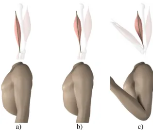
Figure 2. Influence of our muscle deformations on Implicit Skinning. Start-ing from an input pose (a), the muscle is activated (b) and the arm flexed (c). All along, the primitives preserve their volumes and are deformed to avoid collisions. The shape of the muscle central line (in green) is deformed using Position Based Dynamics (PBD) [9].
also includes these deformations and self-contact surfaces by composition of scalar fields fj.
We thus define muscle shapes and dynamics using new field functions fM(Sections 5 and 6), and insert them as additional primitives in the definition of fields fj (Section 7). Muscle primitives are parameterized as follows (see Figure 3):
• two extremity points: the origin m0and the insertion m1, attached relatively to the bones of the animation skeleton and moving kinematically (Section 5.1),
• a set of user parameters to control the muscle geometry, e.g. longitudinal/radial profiles and volume (Section 5.2), • a rest shape, an activated shape, and a shape interpolation
scheme at constant volume to smooth the transition between these two muscle states (Figure 2 and Section 5.2), • a set of particles to simulate elastic deformation of the
muscle, resolve muscle-muscle and muscle-bone collisions and add dynamics effects using Position Based Dynamics (Section 6). pi m0 m1 q C nm0 nm1 fM= 0 θ(q) q cross-sectional view: ni C (s(q)) R(q)
5. Muscle Primitive
The range of shapes that our muscle model produces relies on its adequation to the muscle shapes provided in an anatomic human model [67], the set of muscle shapes and deformations currently used in the computer graphics literature [68, 37], and the capacity of the representation to satisfy our technical (col-lisions, insertion in the Implicit Skinning) and performance requirements.
We propose a formulation producing fusiform muscles defined by swept primitives with a minimal number of user parameters: two parameters for the longitudinal and one for the radial profile, with a scaling parameter. Our model is able to change from rest to activation shape at constant volume. More complex muscles are represented by combining multiple primitives, as explained in Section 5.3. We present the details of our muscle model in this section and discuss the user parameters in Sections 8.3 and 8.4. 5.1. Model
We initially define a muscle M as a scalar field fM: R3→ R constructed by sweeping a profile function R along a central polyline C (see Figure 3 for notations). We design fM as a smooth distance field with 0-isovalues describing the muscle boundaries.
The evaluation of fMat a point q consists of three steps de-tailed below: construction of the central polylineC , projection of q onC to compute the distance d(q, C ), and evaluation of the sweeping profile function R(q). The value of the scalar field at any point q is then given by
fM(q)= d(q, C ) − R(q). (1) Central polyline construction.. The two endpoints m0and m1of the muscle primitive are each attached to an animation bone, so they move kinematically during the animation. The line segment [m0, m1] is divided into N parts with intermediate control points pi. The resulting polylineC is parameterized by s ∈ [0, 1], and we denote as s(q) the curvilinear parameter of the projection of q onC . In order to model muscles with elliptic profiles, the polyline is oriented at each endpoint by given normal vectors nm0and nm1. We associate to each control point of the polyline
pia normal vector ni, defined as follows:
1. we compute an interpolated normal vector by spherical lin-ear interpolation of the normal vectors of the two endpoints, 2. we project this interpolated vector on the plane spanning pi−1, piand pi+1to account for the local twist of the polyline. If these three points are aligned, we interpolate the normals of the two closest polyline control points for which they are defined.
The polyline normal at s(q) is then computed by spherical linear interpolation of the control point normals ni, ni+1of the polyline segment it belongs to.
Projection operator and distance to polyline.. The projection of a query point q onC is a critical step of our approach, as it shapes the properties (e.g. continuity) of the distance function
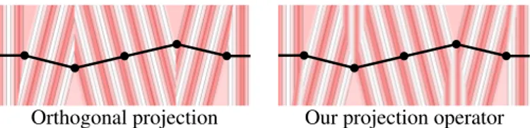
Orthogonal projection Our projection operator
Figure 4. Comparison between standard point-to-segment orthogonal pro-jection, and ours. Colors are computed w.r.t. the curvilinear axis s(proj(q)). Note the discontinuities appearing when using standard orthogonal projec-tion.
d, and thus the primitive scalar field (see Eq. 1). The distance function d is defined as follows:
d(q,C ) =
q − proj(q,C ) 2.
As shown in Figure 4 (left), projecting the query point on the closest segment yields discontinuities in the interior regions of the dihedral angles formed by the segments of the polyline. Similar problems arise also with interpolation on triangle meshes [69, 70]. pi pi+1 pi+2 hi hi+1 λi+1 λi q
We fix this problem by reparam-eterizing the projection on the ar-eas where a point q projects on the interior of two consecutive seg-ments using the cotangent of the angles λiand λi+1formed between the point and the two segments, as
illustrated in the right inset. The projection algorithm is detailed in algorithm 1. As shown in Figure 4 (right), our operator does not exhibit discontinuities and allows projection onto the poly-line vertices even in the interior regions of the dihedral angles formed by the segments of the polyline.
Algorithm 1 Reparameterization of the polyline projection for all segments [pi, pi+1] ofC do
compute hi, the nearest point from q to the segment and si its parameter
end for
Let h be the nearest point from q among all hi, and sh its parameter.
if ∃i such as ((h = hi or h = hi+1) and (none of hi, hi+1 belongs to {p0..pN} )) then
s(q)= sicot λi+si+1cot λi+1
cot λi+cot λi+1
else s(q)= sh end if
return C (s(q))
Sweep surface. The sweep surface is defined by “sweeping” a profile function R(q) alongC . In order to describe the overall shape of fusiform muscles, we parametrize R(q) w.r.t.
• s(q), the curvilinear parameter,
• θ(q), the angle between the polyline normal at s(q) and the vector q − proj(q,C ) (Figure 3).
We specify R to be separable to enable easy evaluation of the muscle’s volume, i.e.,
R(q)= w Φ (s (q)) r (θ (q)) , (2) whereΦ(s) represents the distribution of mass along the axis, r represents the polar profile of the muscle and w is a width scale factor. A sufficient condition for the muscle volume to remain constant is ensuring thatR01(Φ(s))2 ds andR02π(r(θ))2 dθ are constants, as will be shown in the next section. We define our functionsΦ and r so that these integrals both equal 1.
5.2. High level shape parameters
The shape of our muscle primitive is defined by the muscle central polylineC , the scale factor w, and the two sweeping functions r andΦ. In this section we discuss how these parame-ters offer control over 1) the muscle volume, 2) the longitudinal and radial shape profiles, 3) rest/activation muscle shapes. Pa-rameters controlling the muscle shape are detailed in Section 8.4. Volume. WhenC is a straight line we can evaluate the volume of the muscle in cylindrical coordinates as
V= Z 1 s=0 Z 2π θ=0 Z wΦ(s)r(θ) ρ=0 ρdρ dθ lds = πw 2l, (3)
where l is the length of the polylineC (see the derivation details in Appendix A). When the muscle length l changes during the animation, we simply recompute the scale w = √V/πl in Equation 2. This makes the muscle inflate when it contracts and shrink when it is stretched, with constant volume (see Figure 2, top row). Our volume computation is global and performed on a straight polylineC , it thus becomes approximate when C is curved. In practice the volume loss due to the polyline curvature is indiscernible (around 1-3% in our experiments, see Section 8.2). Note that local computations could be considered for a more accurate volume conservation, but this would involve significant computations for a very subtle effect on our muscle parameters adjustment.
Shape longitudinal profile. We defineΦ, the distribution of mass along the muscle axis, as
Φ(s) = ϕ(α, β; s),
where α, β are scalar parameters controlling the shape of the profile. Our definition of ϕ is inspired by the Euler beta func-tion, as it provides geometric profiles similar to muscle shapes. According to Equation 3, volume conservation is guaranteed when the integral of the square of our base function is constant, regardless of α and β. We thus define
ϕ(α, β; s) = ϕ0(α, β; s) kϕ0(α, β; s)k2 where ϕ0is defined for s ∈ [0, 1] as
ϕ0(α, β; s)= sα−1(1 − s)β−1.
e= 0 e= 0.5 e= 0.7 e= 0.9
Figure 5. Elliptic profiles at constant area for different values of the ellipse eccentricity e.
As such, ϕ(α, β; s) can be explicitly written as ϕ(α, β; s) = q sα−1(1 − s)β−1
R1 0 y
2(α−1)(1 − y)2(β−1)dy
. (4)
In principle, α and β can be any positive numbers. For muscle profiles we consider only integer values for efficiency of eval-uation. We additionally impose α > 1 and β > 1 to yield a function where ϕ(0)= ϕ(1) = 0, and α ≤ 9 and β ≤ 9, larger values leading to very sharp profiles that do not correspond to realistic muscle shapes. Note that the denominator of Equation 4 is independent of s and can be pre-computed for all allowed values of α and β using the Euler beta function.
The ratio α/β controls the asymmetry of the shape (with the distribution being symmetric for α = β) while the individual values of α and β control the sharpness of the function’s rise on each side, as illustrated by Figure A.16 in the Appendix. Shape radial profile. In our muscle representation, the radial profile is elliptic and controllable by a single parameter, the ellipse eccentricity e as illustrated in Figure 5. Formally, we set rto be an ellipse of semi-axis lengths u and v:
r(θ)= p uv
u2cos2θ + v2sin2θ
. (5)
The ellipse parameters u and v are directly computed from the eccentricity e so that the product uv = 1 (i.e., the area of the ellipse is always equal to that of a circle of radius 1):
u=p4(1 − e2) v= 1/u.
Rest and activation shapes. When modeling a muscle, there are two shapes to control the muscle state during the animation: the rest shape corresponding to a relaxed state of the muscle fibers and the activation shape corresponding to an increase of tension in the muscle fibers. As illustrated in Figures 2(a) and 2(b) changing of state does not require a change in muscle length, it is an abrupt modification of muscle shape (i.e longitudinal and radial profiles) that can be smoothed over a small sequence of frames by an interpolation at constant volume.
We propose to model this change of muscle state by inter-polating between the two sets of shape parameters (α0, β0, e0) and (α1, β1, e1). We use a ∈ [0, 1] to denote the interpolation parameter. By convention, the rest shape of the muscle corre-sponds to a= 0, and full activation to a = 1. While parameters e0and e1are linearly interpolated, we need to re-normalize the interpolation of the pairs α0, β0and α1, β1 to preserve volume. This is done as follows:
Φ(s) = (1 − a)ϕ(α0, β0, s) + aϕ(α1, β1, s) √
2 1 0 a=1 a=0 a=0.2 a=0.4 a=0.6 a=0.8 0.5 1 0.5 1 0.5 1 0.5 1 0.5 1 0.5 1
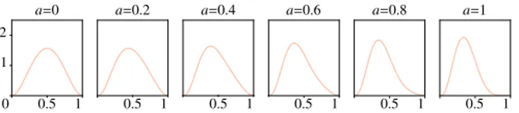
Figure 6. Profiles of theΦ function for α0= β0= 3 and (α1, β1)= (4, 7).
where
F(a)= Z 1
0
((1 − a)ϕ(α0, β0; s)+ aϕ(α1, β1; s))2ds. While the value of F might appear to be expensive to compute for each a, it can be formulated as
F(a)= (1 − a)2+ a2+ 2a(1 − a) K(α0, α1, β0, β1), where K is a constant term which can be expressed in terms of the Euler beta function B
K(α0, α1, β0, β1)=
B(α0+ α1− 1, β0+ β1− 1) pB(2α0− 1, 2β0− 1)B(2α1− 1, 2β1− 1) (see derivation in Appendix B). In practice, K can be precom-puted and tabulated in preprocessing, resulting in fast runtime evaluations. Figure 6 shows an example family of functionsΦ at various levels of interpolation a .
5.3. Extension to non-fusiform muscles
This model produces fusiform muscles such as biceps brachii of the upper limb or quadriceps from the lower limb. To model more complex muscles such as the pectoralis major, we follow a method similar to the one proposed by Scheepers et al. [57] and Murai et al. [71]. We represent these muscles by instancing several fusiform shapes, each integrating a set of muscle fibers. Figure 7 shows an example of pectoral and shoulder muscles. Depending on the desired deformation effects, muscle collisions can be ignored (Figure 7 between green muscles) or enabled as explained in Section 6.3 (Figure 7 between blue muscles).
Figure 7. Pectoral (green) and shoulder (blue) muscles represented by sets of fusiform fibers. In this case, shoulder muscles collide against each other, while the pectorals are allowed to overlap to better approximate the desired shape.
6. Dynamic Muscle Deformations
In Section 5 we have introduced a purely kinematic model for muscles, which deforms at constant volume and whose shape is controlled by high level user parameters. In this section, we show how we extend this model (Section 6.1) to deform the muscles according to their reaction to the animation motion, e.g. muscle jiggling (Section 6.2), and their surroundings: other muscles, bones, or skin (Section 6.3).
6.1. Deformation modeling
To imbue muscles with dynamic behavior, we deform their shape by letting the control points piof the central polylineC be driven by physics-based simulation. While the two extremities m0and m1ofC still follow the kinematics of their skeleton, each internal point piis represented by a particle animated by Position Based Dynamics (PBD) [9]. Thus the muscle elastic-ity and collisions are expressed as constraints solved with the standard PBD Gauss-Seidel solver. This solver iterates on each constraint sequentially yielding a correction applied to the parti-cle’s position (see Figure 8). A strong benefit of our approach is that muscles are defined by 3D scalar fields, which yields very efficient distance queries and allows to interactively resolve collisions (Section 6.3), even for a large number of constraints and particles.
6.2. Muscle elasticity and animation-induced motion
The mass of the whole muscle is set by computing its initial volume multiplied by the average density of muscle tissues ρM= 1.06 g.cm−3[72]. Each moving particle of the muscle’s axis is assigned a fraction of this mass proportionally to the width of the muscle at their initial position on the axis.
The axis particles are tied together by elastic distance con-straints which act as springs in the PBD framework. Each of these constraints is parameterized by its rest length l0and sti ff-ness k. The rest length is set as l0 =2% of the initial distance between the central particles, to provide tension to the muscle axis. A rest length of l0 =100% is assigned to the first 10 % of the length of the muscle at each extremity to represent the more rigid tendons linking the muscle to the bones. The stiffness values k controls the strength of the muscle tone. As discussed in Section 8, in our setup a value of k ≈ 0.1 generates a muscle following the motion of its attachment bones with lots of inertial effects, while a value of k ≈ 0.7 produces a very tense muscle (almost no inertial effects).
6.3. Collision resolution
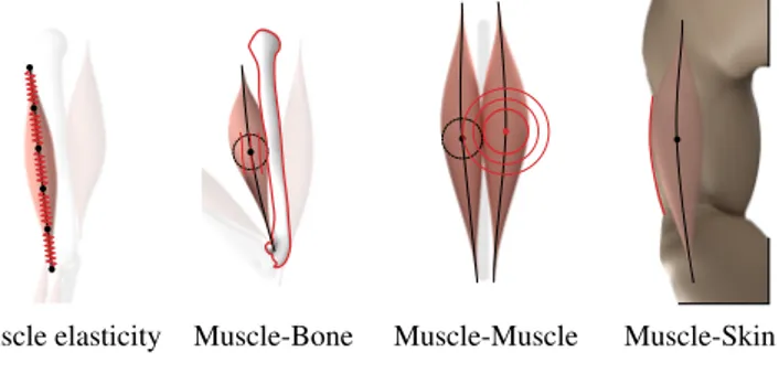
In our body, the shape of muscles is constrained by the pres-ence of rigid bones, other muscles, soft tissues, and skin. To gen-erate more plausible muscle deformations and to better capture the effect of volume preservation, it helps to resolve collisions among the individual organs. The use of scalar fields in con-junction with PBD provides an efficient framework for collision resolution.
Muscle elasticity Muscle-Bone Muscle-Muscle Muscle-Skin
Figure 8. Constraints used to model muscle properties and interactions with surrounding elements.
Muscle-bone collision. We resolve muscle-bone collisions by constraining the particles to stay above a certain radius from the bones. To do so, each particle behaves as a sphere which collides against the bone surface. The collision radius of the particles piis set as wΦ(pi), that approximates the average radius of the muscle’s surface. Since the muscle’s shape evolves during the animation, this radius has to be updated every frame before the PBD solver is executed. The distance between particles and bones is computed efficiently using precomputed distance fields associated with bone shapes (as illustrated in Figure 2) or analytically computing the distance to cylindrical bone proxies (Figure 1).
Muscle-muscle collision. We optionally model collision be-tween muscles in a similar fashion, by constraining the particles of one muscle against the distance field fMof another muscle. This feature is useful for modeling complex muscles consisting of multiple parts that would otherwise overlap.
Muscle-skin interaction. To represent the effect of the skin en-closing the muscles, we add a third field-based constraint to keep the particles themselves inside the 0.5-isosurface of the nearest HRBF field (see Section 7 for the integration of our muscle primitives with the initial HRBF fjin the Implicit Skin-ning framework). This is especially useful for muscles whose shape runs astride a complex joint such as the pectoral across the shoulder, since the tendency of the axis is to form a straight line outside the body. It also prevents inertial effects from dragging the particles outside of the skin in fast motions such as jumping or running.
Regularization. Additionally, to model the visco-elastic prop-erties of biological soft tissues, we introduce a global damping coefficient µ of 0.9 on the velocities at each integration step of the PBD solver. This damping models resistance due to interac-tions of the muscles with other soft tissues (e.g. fat) and prevents long-term muscle vibrations by dissipating their velocity. Also, similarly to rigid-body PBD [73], we add a tangential friction term for each particle which collides against a bone or a mus-cle. This friction force is opposed to the current velocity of the particle, simulating the loss of energy when the two anatomical objects interact.
7. Integration with Implicit Skinning 7.1. Composition operators
As explained in Section 4, the dynamic deformations of our muscles have to be included in the scalar fields fj(defined by HRBF) before they are composed to produce the final field f whose 0.5-isosurface represents the skin.
The field representation fMintroduced in Section 5 is a dis-tance field with a global support. Implicit Skinning relies on compactly supported field functions and an homogeneous for-mulation is required to adequately integrate our functions [63]. We thus convert our muscles to compact support by composing
fMwith a fall-off transfer function as done for the HRBF fields described by Vaillant et al. [7]. We then assemble together all muscular fields associated with a given animation bone with a union operator before blending them with the HRBF to produce the new fields fj.
The mesh tracking step of Implicit Skinning (Section 3) relies on a gradient descent in the field f . Gradient directions should thus be smooth and singular points (where ∇ f = 0) in tracking areas must be avoided. The standard max union operator on field functions [75, 76] is known to produce gradient discontinuities and we rather compose muscles with clean union operators [77, 78] that generate a smoothed gradient. The blending of the assembled muscles with the HRBF introduces singular points along the muscle axis in the fields fj. It also produces gradient directions pointing to the bone rather than the skin in the bone-facing part of muscles as illustrated in Figure 9-center. This problem in implicit modeling has been raised by Canezin et al. [74] when small details are added to a large object with a blending operator. The solution is to use the detail blending operator of Canezin et al. [74] that blends only the outside part of the muscle without including the central singular points and the bone-facing parts in the resulting field, as illustrated in Figure 9-right.
During the animation, we want the skin to capture the underly-ing muscle’s shape when it bulges out but also when it contracts. In our approach, muscles are added to the initial HRBF skin approximation using a blending operator (union with a smoothed transition between the combined objects). This means that if the muscle deforms completely inside the HRBF, it will not modify its shape, leaving the skin represented by fjunchanged. In order to deform the skin shape fjwith all visible muscle deformations, we reduce the HRBF surface along muscles so that it represents a muscular rest surface. The blending of the muscle primitives then locally adds the muscle shapes in the limb representation, and the skin shape in this area follows the deformations of the muscles.
7.2. Integration in the Implicit Skinning pipeline
Figure 10 illustrates the framework to follow for the produc-tion of an animaproduc-tion frame. At each new frame, the animaproduc-tion skeleton is transformed to its new position. Data which is kine-matically bound to the animation bones, such as the individual HRBF fields, the muscles endpoints and the scalar fields rep-resenting the rigid bones are updated. Keyframed per-muscle shape parameters (eccentricity, activation and width exaggera-tion) are also updated during this stage.
setup with union operator with detail operator
Figure 9. Left: a typical skinning setup with muscles and bone primitives blended with the HRBF field. Center: using a union operator yields singular points (red dotted line) and wrong gradient directions (red arrows) near the 0.5-isosurface. Right : the use of Canezin et al. [74] detail blending operator (right) avoids these problems, eliminating the singular points and yielding a smooth gradient.
Animation Compute relative
transformations
Mesh Update
Transform HRBFs Transform
Muscles ends Update MusclesParameters PBD
Update Primitives Mesh Tracking
Standard animation Implicit Skinning Muscles primitives (ours)
Figure 10. Breakdown of the Implicit Skinning pipeline with muscles. Steps pictured in grey are the standard geometric skinning pipeline, steps in brown are the Implicit Skinning correction algorithm and steps in salmon are our new anatomic-related workflow. Each arrow represents a direct dependency between steps.
Next, the PBD solver computes the new position of the parti-cles. The PBD timestep can be set to a fraction of the animation framerate, which yields an overall stiffer behavior of the physics engine. After the new particle positions are computed, each mus-cle updates its sampled normals nias described in Section 5.1 and scales its width according to the new length of its axis, as explained in Section 5.2. All underlying field functions are now set and the final skin field f is ready to be evaluated by the Implicit Skinning tracking to skin the character mesh vertices.
8. Results and discussions
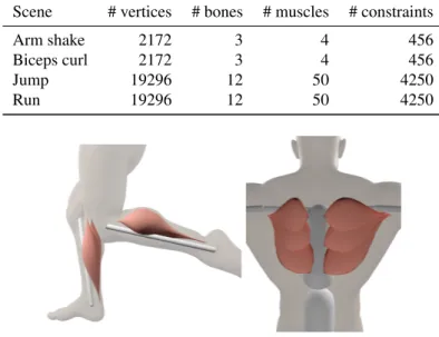
We set up a variety of scenes ranging from simple motions, such as an arm shake or a biceps curl (involving only a few muscles) to challenging motions, such as jumping and running with a fully rigged model. Please see Table 1 for details.
Results were generated on a 3.6 GHz Intel Xeon E5-1650 CPU with 64 GB of memory. Our method does not add
signifi-Table 1. Summary of the scenes used for our results. The number of PBD constraints is given for 30 particles per muscle.
Scene # vertices # bones # muscles # constraints
Arm shake 2172 3 4 456
Biceps curl 2172 3 4 456
Jump 19296 12 50 4250
Run 19296 12 50 4250
Figure 11. Calf muscles in their least activated state (left;α0= β0= 3, a =
0) and their most activated state (right; α1 = 4, β1 = 8, a = 1). Dorsal
muscles are shown in their rest state (α0= 2, β0= 3).
cant memory overhead to Implicit Skinning due to the compact representation of muscles in memory. The blending operator of Canezin et al. [74] and the optional cached distance fields for anatomic bones are the only memory overhead required for adding our muscle deformations. This represents less than 200 KB for the operator and 8 MB per optional anatomic bone.
The default shape setting for our muscles is α0 = β0 = 3 and α1 = 4, β1 = 7, yielding a smooth symmetric shape in its inactivated state and a significant bulge in its fully activated state, as depicted in Figure 11, left. Other shapes are also used in large flat muscles such as dorsals (α0= 1, β0= 3) (Figure 11, right) or pectorals (α0= 3, β0= 9) (Figure 7).
The stiffness of the distance constraints between the particles affects mostly the inertial motion of the muscle: stiff muscles (k = 0.6) tend to closely follow the skeleton’s motion while
Table 2. Average times in seconds per frame for our different scenes and 30 particles per muscle. Times are given for Implicit Skinning without muscles (IS only), for Implicit Skinning with muscles but without the PBD simulation (IS), and for the PBD simulation (PBD).
Scene Standard IS IS+ Muscles
Tracking PBD Total
Arm shake 0.008 0.013 0.055 0.068
Biceps curl 0.005 0.015 0.042 0.057
Jump 0.050 0.462 0.096 0.558
Run 0.051 0.473 0.096 0.569
softer muscles (k= 0.1) tend to drag and jiggle much more.
8.1. Timings
Table 2 shows the average time per frame for each of our scenes. For reference, we included the time per frame of standard Implicit Skinning without muscles. While Implicit Skinning runs at real-time frame rates even in more demanding scenes, adding more muscles or increasing the number of particles per muscle increases both the physics solver time and the run-time of the Implicit Skinning algorithm itself. The former happens because more constraints have to be solved, while the latter occurs be-cause the Implicit Skinning algorithm has to evaluate the muscle fields several times for the neighboring vertices. Nevertheless, even with our most complex scene with 50 muscles each in-cluding 30 particles, we maintain a total frame time below one second.
When editing the muscle parameters it is possible to disable Implicit Skinning to have interactive response times (up to 5-6 fps for the jumping model with the physics of all muscles acti-vated). The parameters of each individual muscle can be tuned in real time, taking advantage of the fact that only one muscle is edited. Also, muscles subject to small deformations can be represented by fewer particles, which reduces the number of constraints and increases the simulation speed while decreasing the evaluation cost of the muscle scalar fields (see Figure 12). Note that even though subtle in Figure 12-left, the muscle scalar field computation time increases with the number of particles. This increase is due to the larger number of segments to consider for the evaluation point projection on the muscle polyline (see Section 5.1).
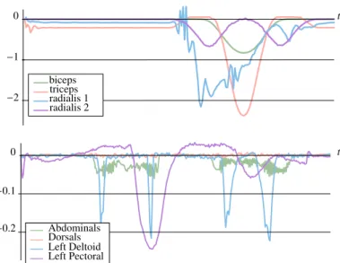
8.2. Volume conservation
We measured experimentally the volume variation of our mus-cle models due to the bending of the central axis (see Section 5). Figure 13 shows the variation of a numerical approximation of the volume of different muscles during the biceps and the jump animations (using the volume of the representative mesh as a proxy). The highest variation is approximately 3%.
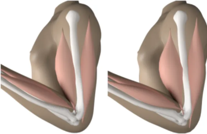
Our model also allows a user to transgress this volume con-straint to amplify the muscle growth for expressive effect by tuning the scale factor w of the muscles as shown in Figure 14.
Implicit Skinning PBD Simulation 1.5 1 0.75 0.5 0.25
Arm shake Jump
0 5 10 20 30 60 t 0 5 10 20 30 60 1.5 1 0.75 0.5 0.25 t # particles # particles
Figure 12. Average times in seconds for the computation of an animation frame, for different numbers of particles per muscle. The brown represents the computation of Implicit Skinning excluding the PBD simulation, and the pink represents the PBD simulation.
biceps triceps radialis 1 radialis 2 0 −1 −2 t t 0 −0.1 −0.2 Abdominals Dorsals Left Deltoid Left Pectoral
Figure 13. Relative variation over time (in %) of muscles volume during, top - the biceps curl and bottom - the jump animation.
Figure 14. Left, normal biceps curl. Right, muscle width increased by 30%.
8.3. User parameters
Our model exposes two sets of muscle parameters, i.e. the geometric parameters and the dynamic parameters, and a muscle state, i.e relaxed and activated.
8.3.1. Geometric parameters
Geometric parameters are introduced in Section 5.2 with our volume equations. They are α and β for the muscle longitudinal shape, the eccentricity e for its radial cross-section, and the scale factor w.
As shown in Figure A.16, the value of α and β, from 2 to 9, control the position of the bulge along the axis and the sharpness of its rise on each end of the axis. The shape is symmetrical when α= β, with higher values corresponding to a narrower bulge. The more the values differ, the further the maximum point is from the axis center.
The eccentricity parameter produces circular radial shapes when e= 0 and smoothly interpolates towards more elongated elliptic cross-sections when it approaches 1, as illustrated in Figure 5. Note that this parameter has a non linear impact on the ellipse dimensions. This can easily be compensated by adjusting the input value provided by the user, for instance when using a slider moving from circular to flat.
The last geometric parameter, w controls the uniform scale over the muscle width to adjust its global size.
8.3.2. Muscle activation
Two different shapes of a muscle can be defined using the geometric parameters α, β, e and optionally w: the muscle rest shape, and the activated state. A muscle activation is in gen-eral almost instantaneous and the muscle may change its shape from rest to activation in a few frames. Our model can vary continuously from one shape to the other using the muscle shape interpolation at constant volume introduced in Section 5.2. Once these two shapes are set, the muscle state and its corresponding shape are defined by the interpolation parameter a with a= 0 for the rest state and a= 1 for the fully activated shape. 8.3.3. Dynamic parameters
To be deformed in response to the skeleton motion as ex-plained in Section 6, each muscle is parametrized by its mass,
its rest length and its stiffness k. The PBD solver is also con-trolled by global parameters: the timestep δt and the damping coefficient µ. The mass, rest length and damping parameters are preset as explained in Sections 6.2 and 6.3. Changing the global engine parameters is a possibility to access a wider variety of motions, but this requires adjusting the stiffness of every muscle in the scene to keep the muscles’ behavior consistent. This is a limitation of the PBD approach that is discussed further in Section 8.6 and we thus suggest to avoid the modification of these paramters.
In our experiments, we thus only provide a single dynamic user parameter, the stiffness k, to adjust per-muscle to obtain a stiffer or looser behavior of a given muscle.
8.4. Parameter setting 8.4.1. Keyframing parameters
Keyframing is a standard approach for controlling parameters over an animation. All the geometric parameters and the stiffness can be keyframed in order to allow the user to have a maximal control of the deformations. We linearly interpolate the eccen-tricity e, interpolation a, scaling w and the stiffness k while α and β are interpolated with our interpolation at constant volume (see Section 5.2). If required, any higher degree interpolation may be used for e, w and k.
8.4.2. User parameter setting
The parameters can be set in an interactive muscle modelling session, using standard UI controllers such as sliders for the continuously varying values e, w and k, and a set of icons for automatically selecting the values of α and β. Common muscles of a body may also be preset, together with their activated shape and directly proposed to the user that just have to adjust the endpoint positions and the scaling w, optionally tweaking the other parameters.
Once both rest and activation shapes are set, the interpolation parameter a can be keyframed by the user or automatically set if forces information is provided by the animation system.
In our experiments, the manual edition of a muscle geometric parameters including rest and activation shapes in a prototype script interface takes around 10 minutes and the keyframing of the muscle state interpolation a and its stiffness k takes a few minutes for about a minute of animation. The use of a dedicated UI as the one provided in a professional software would greatly lower these timings by enabling the setting of individual muscles in an interactive visual session.
8.4.3. Automatic parameter setting
One may consider automatic adjustment methods to set the muscle parameters, for example by adapting existing anatomi-cal models with Anatomy Transfer [79]. Another direction of investigation is to use a data-based approach to set the muscle shape parameters from sparse motion capture marker inputs, by optimizing the muscle activation parameters as proposed by Sifakis et al. [80]. Similarly, muscular activity models such as the locomotion model of Lee et al. [81] can control the evolution of muscle activation parameters.
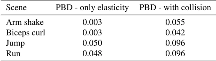
Table 3. Average times in seconds per frame for minimizing PBD constraints, without and with collision constraints (muscle/bones, mus-cle/muscle, interactions with skin), in our different scenes.
Scene PBD - only elasticity PBD - with collision
Arm shake 0.003 0.055
Biceps curl 0.003 0.042
Jump 0.050 0.096
Run 0.048 0.096
8.5. Effects of collisions
As shown by Table 3, the addition of collision constraints in the PBD solver doubles its convergence time on a full model. However, the use of collisions is mandatory as without them, two main phenomena occur. The first is that a significant part of the muscle grows inside the bone and neighbor muscles when it inflates. This cancels most of the inflation effect naturally produced on the skin by the muscle volume preservation and thus significantly reduces the deformation plausibility, as illustrated in Figure 15 and in the accompanying video. The second is the unnatural behavior of muscles that are allowed to move through where the bones should be, instead of moving around them (for instance on a shoulder).
Figure 15. The arm bent from left to right with Implicit Skinning only, with our muscle but without resolving muscle/bones collisions and with our muscles and muscle/bones collisions resolved. Without collision, the muscle deformation in the middle is very similar to the solution without muscle shown on the left. On the right, the collision makes the muscle deformation clearly visible.
8.6. Muscle dynamics
Even though PBD is appreciated for its robustness, fast execu-tion, and ease of implementaexecu-tion, there are also certain trade-offs. One issue is the dependence between the time integration step and the stiffness of the constraints: larger time steps yield softer constraints, thus a more rubbery material. This issue could possi-bly be avoided using the method proposed by Macklin et al. [82], as it could improve predictability of the results with different time steps.
Projective Dynamics [83] have been considered in place of PBD. It averages all constraint projections in one global step which limits oscillations. However, the pre-factorization of the global step matrix in Projective Dynamics complicates colli-sion resolution, especially in close proximity scenarios such as muscle-bone or muscle-muscle scenarios. Therefore, we have for now decided not to pursue this approach.
Unless muscles are set with a too low stiffness, which is un-realistic as muscles are stiff organs compared to soft tissues, especially when activated, the muscle dynamic is stable or most muscles (as pectorals, biceps, triceps muscles) even with mus-cle/bones and muscle/muscle collisions enabled. Some difficul-ties may arise when muscles undergo large deformations due to collisions. In this case collisions are strongly contradicting the muscle elasticity and undesired oscillations may arise. In such situations, our solution is to pinch the muscle between two other muscles (as a small decomposition in fibers) and increase the stiffness. This is a limitation of our model under its current form that would be interesting to solve in further research.
Another limitation when using PBD is that the jiggling of muscles may be hard to generate. While simple oscillations are easy to obtain (such as the one shown in the video on the biceps when shaking the arm), it is far more challenging to generate plausible longitudinal jiggling as those expected on muscle legs during a run, even acting on all PBD parameters. This is partially due to the use of a dynamic system based on constraints rather than forces.
8.7. Integration in other skinning frameworks
On the one hand, while our muscle primitives have been specifically designed to enrich the Implicit Skinning ap-proach [8], they may benefit weight-based geometric skinning techniques [58, 59, 61]. In these systems, a set of weights is defined over the mesh for each muscle. Mesh vertices with non-zero weights store the initial field value of the corresponding muscle primitives in rest pose. During the animation, muscle deformation and skinning are performed. Then, for each vertex with non-zero weight, a displacement corresponding to its pro-jection on its initial field value in the deformed muscle field is computed (using for instance a gradient descent). Vertex posi-tions are then updated by applying the weighted displacements. On the other hand, real-time physically or dynamic based skinning methods, such as position-based skinning [84], usually rely on a volumetrical mesh deformed by minimizing a function defined by constraints. In that case, the definition and insertion of constraints transferring the muscle field function deformations on the volumetrical mesh remains an open challenge. In addition, the interaction of these new constraints with the others will also have to be specifically studied, especially because some of them may violate each other. A way to avoid these issues is to apply the muscle deformations as a post-process, but all physical properties and eventual collision-handling would be lost. 8.8. Limitations
As can be seen in Figure 12, computations required by Im-plicit Skinning are the main bottleneck for a full model. This is due to the very large number of field functions that are struc-tured in a composition tree [85] and evaluated several times per mesh vertex for the isosurface tracking. This phenomenon is accentuated by the increased number of deformed vertices due to the muscle dynamics. Even though we use a bounding box hierarchy to avoid unnecessary field evaluations, there is room for specifically improving the field function filtering and
composition tree evaluations. We currently rely on a CPU im-plementation which is multi-threaded, but not heavily optimized. Both Implicit Skinning and PBD may be efficiently implemented on a GPU, and it would be interesting to study a dedicated GPU implementation including our muscle primitives.
The variety of muscle shapes produced with our model is well-suited for the production of plausible body dynamics of a human character. The main limitation is the application to non-fusiform muscles as the pectoral, for which we allow the introduction of visible deformations, but we provide a coarse approximation of the muscle shape and the deformations could be enhanced with a more accurate model. Different types of muscle primitives may be studied to adapt to a larger variety of virtual characters, including animals and imaginary creatures.
9. Conclusion
In this paper, we have presented a method to animate a char-acter’s muscular system which achieves expressive, artistically controllable results while maintaining interactive frame-rates.
To achieve this goal, we designed a family of shapes defined as isosurfaces of a scalar field. These shapes mimic the appearance of human muscles and are able to reproduce the contraction, extension, volume preservation and activation of the real muscles. Furthermore, we let the central axis of our muscles be driven by physics-based simulation, thus enabling highly dynamic effects such as jiggling. Using 3D scalar field representation allows us to resolve collisions efficiently between muscles, bones and skin. Another advantage of this implicit representation is the ability to use the muscles as skin deformers while reaping the benefits of Implicit Skinning.
As future work, a sketching approach may be investigated, en-abling users to sketch the muscle deformation in different poses. We also believe that combining physical simulation with implicit modeling for animation is a promising line of research. Indeed, using a similar representation for other anatomic elements with highly dynamic behaviour and effect on the skin such as fat tissues or cartilages (nose, ears) could improve the ability of animators to efficiently produce realistic visual effects.
10. Acknowledgements
This research has been partially supported by the FOLD-Dyn project (ANR-16-CE33-0015-01) and the CIMI Labex (ANR-11-LABX-0040). This material is also based upon work supported by the National Science Foundation under Grant Numbers IIS-1617172, IIS-1622360 and IIS-1764071. Any opinions, findings, and conclusions or recommendations expressed in this material are those of the author(s) and do not necessarily reflect the views of the National Science Foundation. We also gratefully acknowl-edge the support of Activision, Adobe, and hardware donation from NVIDIA Corporation. The authors would like to thank the anonymous reviewers for their helpful comments and sugges-tions. Finally, we wish to thank the Anatoscope company and more specifically Pr Franc¸ois Faure for the gracious provision of their anatomical model.
References
[1] Magnenat-Thalmann, N, Laperrire, R, Thalmann, D. Joint-Dependent Local Deformations for Hand Animation and Object Grasping. In: Pro-ceedings of Graphics Interface. GI 1988; Edmonton, Canada; 1988, p. 26–33.
[2] Kavan, L, Collins, S, ˇZ´ara, J, O’Sullivan, C. Skinning with Dual Quater-nions. In: Proceedings of the Symposium on Interactive 3D Graphics and Games. I3D ’07; Seattle, USA: ACM. ISBN 978-1-59593-628-8; 2007, p. 39–46. URL: http://doi.acm.org/10.1145/1230100.1230107. doi:10.1145/1230100.1230107.
[3] Lewis, JP, Cordner, M, Fong, N. Pose space deformation: A uni-fied approach to shape interpolation and skeleton-driven deformation. In: Proceedings of the 27th Annual Conference on Computer Graph-ics and Interactive Techniques. SIGGRAPH ’00; New Orleans, USA: ACM Press/Addison-Wesley Publishing Co. ISBN 1-58113-208-5; 2000, p. 165–172. URL: http://dx.doi.org/10.1145/344779.344862. doi:10.1145/344779.344862.
[4] Wilhelms, J, Van Gelder, A. Anatomically-based modeling. In: Pro-ceedings of the 24th Annual Conference on Computer Graphics and Interactive Techniques. SIGGRAPH ’97; New York, NY, USA: ACM Press/Addison-Wesley Publishing Co. ISBN 0-89791-896-7; 1997, p. 173–180. URL: http://dx.doi.org/10.1145/258734.258833. doi:10.1145/258734.258833.
[5] Mohr, A, Gleicher, M. Building efficient, accurate character skins from examples. ACM Transactions on Graphics 2003;22(3):562– 568. URL: http://doi.acm.org/10.1145/882262.882308. doi:10. 1145/882262.882308.
[6] Wang, RY, Pulli, K, Popovi´c, J. Real-time enveloping with rotational regression. ACM Transactions on Graphics 2007;26(3). URL: http:// doi.acm.org/10.1145/1276377.1276468. doi:10.1145/1276377. 1276468.
[7] Vaillant, R, Barthe, L, Guennebaud, G, Cani, MP, Rohmer, D, Wyvill, B, et al. Implicit Skinning: Real-time Skin Deformation with Contact Modeling. ACM Transactions on Graphics 2013;32(4):125:1–125:12. doi:10.1145/2461912.2461960.
[8] Vaillant, R, Guennebaud, G, Barthe, L, Wyvill, B, Cani, MP. Robust Iso-surface Tracking for Interactive Character Skinning. ACM Transactions on Graphics 2014;33(6):189:1–189:11. URL: http://doi.acm.org/ 10.1145/2661229.2661264. doi:10.1145/2661229.2661264. [9] M¨uller, M, Heidelberger, B, Hennix, M, Ratcliff, J. Position based
dynamics. Journal of Visual Communication and Image Representa-tion 2007;18(2):109 – 118. URL: http://www.sciencedirect.com/ science/article/pii/S1047320307000065. doi:http://dx.doi. org/10.1016/j.jvcir.2007.01.005.
[10] Mukai, T. Example-Based Skinning Animation. Springer International Publishing; 2016, p. 1–21.
[11] Allen, B, Curless, B, Popovi´c, Z. Articulated body deformation from range scan data. ACM Transactions on Graphics 2002;21(3):612– 619. URL: http://doi.acm.org/10.1145/566654.566626. doi:10. 1145/566654.566626.
[12] Anguelov, D, Srinivasan, P, Koller, D, Thrun, S, Rodgers, J, Davis, J. Scape: Shape completion and animation of people. ACM Transactions on Graphics 2005;24(3):408–416. URL: http://doi.acm.org/10.1145/ 1073204.1073207. doi:10.1145/1073204.1073207.
[13] Allen, B, Curless, B, Popovi´c, Z, Hertzmann, A. Learning a correlated model of identity and pose-dependent body shape variation for real-time synthesis. In: Proceedings of the 2006 ACM SIGGRAPH/Eurographics symposium on Computer animation. Eurographics Association; 2006, p. 147–156.
[14] Park, SI, Hodgins, JK. Capturing and animating skin deformation in human motion. In: ACM SIGGRAPH 2006 Papers. SIGGRAPH ’06; New York, NY, USA: ACM. ISBN 1-59593-364-6; 2006, p. 881–889. URL: http://doi.acm.org/10.1145/1179352.1141970. doi:10.1145/1179352.1141970.
[15] Park, SI, Hodgins, JK. Data-driven modeling of skin and mus-cle deformation. ACM Transactions on Graphics 2008;27(3):96:1– 96:6. URL: http://doi.acm.org/10.1145/1360612.1360695. doi:10.1145/1360612.1360695.
[16] Neumann, T, Varanasi, K, Hasler, N, Wacker, M, Magnor, M, Theobalt, C. Capture and statistical modeling of arm-muscle deformations. Computer Graphics Forum 2013;32(2):285–294.
[17] Loper, M, Mahmood, N, Black, MJ. Mosh: Motion and shape capture from sparse markers. ACM Transactions on Graphics 2014;33(6):220. [18] Tsoli, A, Mahmood, N, Black, MJ. Breathing life into shape: capturing,
modeling and animating 3d human breathing. ACM Transactions on Graphics 2014;33(4):52.
[19] Loper, M, Mahmood, N, Romero, J, Pons-Moll, G, Black, MJ. SMPL: A skinned multi-person linear model. ACM Transactions on Graph-ics 2015;34(6):248:1–248:16. URL: http://doi.acm.org/10.1145/ 2816795.2818013. doi:10.1145/2816795.2818013; proceedings of SIGGRAPH Asia.
[20] Mukai, T, Kuriyama, S. Efficient dynamic skinning with low-rank helper bone controllers. ACM Transactions on Graphics 2016;35(4):36:1– 36:11. URL: http://doi.acm.org/10.1145/2897824.2925905. doi:10.1145/2897824.2925905.
[21] Pons-Moll, G, Romero, J, Mahmood, N, Black, MJ. Dyna: A model of dynamic human shape in motion. ACM Transactions on Graph-ics 2015;34(4):120:1–120:14. URL: http://doi.acm.org/10.1145/ 2766993. doi:10.1145/2766993.
[22] Kim, M, Pons-Moll, G, Pujades, S, Bang, S, Kim, J, Black, MJ, et al. Data-driven physics for human soft tissue animation. ACM Transactions on Graphics 2017;36(4):54:1–54:12. URL: http://doi.acm.org/10. 1145/3072959.3073685. doi:10.1145/3072959.3073685.
[23] Schneider, DC, Davidson, TM, Nahum, AM. In vitro biaxial stress-strain response of human skin. Archives of Otolaryngology 1984;110(5):329– 333. URL: +http://dx.doi.org/10.1001/archotol.1984. 00800310053012. doi:10.1001/archotol.1984.00800310053012. [24] Girard, M, Maciejewski, AA. Computational modeling for the
com-puter animation of legged figures. In: Proceedings of the 12th An-nual Conference on Computer Graphics and Interactive Techniques. SIG-GRAPH ’85; New York, NY, USA: ACM. ISBN 0-89791-166-0; 1985, p. 263–270. URL: http://doi.acm.org/10.1145/325334.325244. doi:10.1145/325334.325244.
[25] Chadwick, JE, Haumann, DR, Parent, RE. Layered construction for deformable animated characters. SIGGRAPH Computer Graphics 1989;23(3):243–252. URL: http://doi.acm.org/10.1145/74334. 74358. doi:10.1145/74334.74358.
[26] Zajac, FE. Muscle and tendon: properties, models, scaling, and applica-tion to biomechanics and motor control. Critical reviews in biomedical engineering 1989;17 4:359–411.
[27] Chen, DT, Zeltzer, D. Pump it up: Computer animation of a biomechani-cally based model of muscle using the finite element method. SIGGRAPH Computer Graphics 1992;26(2):89–98. URL: http://doi.acm.org/ 10.1145/142920.134016. doi:10.1145/142920.134016.
[28] Teran, J, Blemker, S, Ng-Thow-Hing, V, Fedkiw, R. Finite vol-ume methods for the simulation of skeletal muscle. In: Proceedings of the 2003 ACM SIGGRAPH/Eurographics Symposium on Computer Animation. SCA ’03; Aire-la-Ville, Switzerland, Switzerland: Euro-graphics Association. ISBN 1-58113-659-5; 2003, p. 68–74. URL: http://dl.acm.org/citation.cfm?id=846276.846285.
[29] Teran, J, Sifakis, E, Blemker, S, Ng-Thow-Hing, V, Lau, C, Fed-kiw, R. Creating and simulating skeletal muscle from the visible human data set. IEEE Transactions on Visualization and Computer Graphics 2005;11(3):317–328. doi:10.1109/TVCG.2005.42.
[30] Lee, SH, Sifakis, E, Terzopoulos, D. Comprehensive biomechan-ical modeling and simulation of the upper body. ACM Transactions on Graphics 2009;28(4):99:1–99:17. URL: http://doi.acm.org/10. 1145/1559755.1559756. doi:10.1145/1559755.1559756.
[31] Pai, DK, Sueda, S, Wei, Q. Fast physically based musculoskeletal simulation. In: ACM SIGGRAPH 2005 Sketches. SIGGRAPH ’05; New York, NY, USA: ACM; 2005,URL: http://doi.acm.org/10.1145/ 1187112.1187141. doi:10.1145/1187112.1187141.
[32] Pai, DK. Muscle mass in musculoskeletal models. Journal of Biome-chanics 2010;43(11):2093 – 2098. URL: http://www.sciencedirect. com/science/article/pii/S0021929010002149. doi:http://dx. doi.org/10.1016/j.jbiomech.2010.04.004.
[33] Sueda, S, Kaufman, A, Pai, DK. Musculotendon simulation for hand animation. ACM Transactions on Graphics 2008;27(3):83:1– 83:8. URL: http://doi.acm.org/10.1145/1360612.1360682. doi:10.1145/1360612.1360682.
[34] Sueda, S, Jones, GL, Levin, DIW, Pai, DK. Large-scale dynamic simulation of highly constrained strands. ACM Transactions on Graph-ics 2011;30(4):39:1–39:10. URL: http://doi.acm.org/10.1145/
2010324.1964934. doi:10.1145/2010324.1964934.
[35] McAdams, A, Zhu, Y, Selle, A, Empey, M, Tamstorf, R, Teran, J, et al. Efficient elasticity for character skinning with con-tact and collisions. ACM Transactions on Graphics 2011;30(4):37:1– 37:12. URL: http://doi.acm.org/10.1145/2010324.1964932. doi:10.1145/2010324.1964932.
[36] Patterson, T, Mitchell, N, Sifakis, E. Simulation of complex nonlin-ear elastic bodies using lattice deformers. ACM Transactions on Graph-ics 2012;31(6):197:1–197:10. URL: http://doi.acm.org/10.1145/ 2366145.2366216. doi:10.1145/2366145.2366216.
[37] Fan, Y, Litven, J, Pai, DK. Active volumetric musculoskeletal systems. ACM Transactions on Graphics 2014;33(4):152:1–152:9. URL: http:// doi.acm.org/10.1145/2601097.2601215. doi:10.1145/2601097. 2601215.
[38] Sachdeva, P, Sueda, S, Bradley, S, Fain, M, Pai, DK. Biomechanical simulation and control of hands and tendinous systems. ACM Transactions on Graphics 2015;34(4):42:1–42:10. URL: http://doi.acm.org/10. 1145/2766987. doi:10.1145/2766987.
[39] Gao, M, Mitchell, N, Sifakis, E. Steklov-poincar´e skinning. In: Proceed-ings of the ACM SIGGRAPH/Eurographics Symposium on Computer An-imation. SCA ’14; Aire-la-Ville, Switzerland, Switzerland: Eurographics Association; 2014, p. 139–148. URL: http://dl.acm.org/citation. cfm?id=2849517.2849541.
[40] Saito, S, Zhou, ZY, Kavan, L. Computational bodybuilding: Anatomically-based modeling of human bodies. ACM Transactions on Graphics 2015;34(4):41:1–41:12. URL: http://doi.acm.org/10. 1145/2766957. doi:10.1145/2766957; proceedings of SIGGRAPH 2015.
[41] Kadleˇcek, P, Ichim, AE, Liu, T, Kˇriv´anek, J, Kavan, L. Reconstruct-ing personalized anatomical models for physics-based body animation. ACM Transactions on Graphics 2016;35(6):213:1–213:13. URL: http:// doi.acm.org/10.1145/2980179.2982438. doi:10.1145/2980179. 2982438.
[42] Mohr, A, Tokheim, L, Gleicher, M. Direct manipulation of interactive character skins. In: Proceedings of the 2003 Symposium on Interactive 3D Graphics. I3D ’03; New York, NY, USA: ACM. ISBN 1-58113-645-5; 2003, p. 27–30. URL: http://doi.acm.org/10.1145/641480. 641488. doi:10.1145/641480.641488.
[43] Merry, B, Marais, P, Gain, J. Animation space: A truly lin-ear framework for character animation. ACM Transactions on Graph-ics 2006;25(4):1400–1423. URL: http://doi.acm.org/10.1145/ 1183287.1183294. doi:10.1145/1183287.1183294.
[44] Forstmann, S, Ohya, J, Krohn-Grimberghe, A, McDougall, R. Defor-mation styles for spline-based skeletal aniDefor-mation. In: Proceedings of the 2007 ACM SIGGRAPH/Eurographics symposium on Computer animation. Eurographics Association; 2007, p. 141–150.
[45] Kavan, L, Collins, S, ˇZ´ara, J, O’Sullivan, C. Geometric skinning with approximate dual quaternion blending. ACM Transactions on Graph-ics 2008;27(4):105. URL: http://doi.acm.org/10.1145/1409625. 1409627. doi:10.1145/1409625.1409627.
[46] Jacobson, A, Baran, I, Popovi´c, J, Sorkine, O. Bounded bihar-monic weights for real-time deformation. ACM Transactions on Graph-ics 2011;30(4):78:1–78:8. URL: http://doi.acm.org/10.1145/ 2010324.1964973. doi:10.1145/2010324.1964973.
[47] Jacobson, A, Sorkine, O. Stretchable and twistable bones for skeletal shape deformation. ACM Transactions on Graphics 2011;30(6):165. [48] Kavan, L, Sorkine, O. Elasticity-inspired deformers for
charac-ter articulation. ACM Transactions on Graphics 2012;31(6):196:1– 196:8. URL: http://doi.acm.org/10.1145/2366145.2366215. doi:10.1145/2366145.2366215.
[49] Le, BH, Hodgins, JK. Real-time skeletal skinning with optimized centers of rotation. ACM Transactions on Graphics 2016;35(4):37:1– 37:10. URL: http://doi.acm.org/10.1145/2897824.2925959. doi:10.1145/2897824.2925959.
[50] Sloan, PPJ, Rose III, CF, Cohen, MF. Shape by example. In: Proceedings of the Symposium on Interactive 3D Graphics. I3D ’01; Research Triangle Park, USA: ACM. ISBN 1-58113-292-1; 2001, p. 135–143. URL: http://doi.acm.org/10.1145/364338.364382. doi:10.1145/364338.364382.
[51] Kry, PG, James, DL, Pai, DK. Eigenskin: Real time large de-formation character skinning in hardware. In: Proceedings of the ACM SIGGRAPH/Eurographics Symposium on Computer Animation.