Characterization of Nb₃Sn superconducting strand under pure bending

by David L. Harris

B.S. Mechanical Engineering (2003) Utah State University

Submitted to the Department of Mechanical Engineering in Partial Fulfillment of the Requirements for the Degree of

Master of Science in Mechanical Engineering at the

Massachusetts Institute of Technology September 2005

0 2005 Massachusetts Institute of Technology All right reserved

Signature of Author ... Cr-tified bI Certified by ... Accepted by ... MASSACHUSETTS INSTITU OF TECHNOLOGY

NOV 0 7 2005

LIBRARIES

Department of Mechanical Engineering August 10, 2005

... ... ... ... . .. . .

Joseph V. Minervini Senior Research Engineer, MIT Plasma Science and Fusion Center Nuclear Science and Engineering Department Thesis Supervisor

... ivseph L. Smith, Jr. Samuel C. Collins Seniorjfpfessor of Mechanical Engineering Thesis Supervisor

... ... ...

Lallit Anand Chairman, Department Committee on Graduate Students

E

BARKER y ...

by David L. Harris

Submitted to the Department of Mechanical Engineering on August 10, 2005 in Partial Fulfillment of the Requirements for the Degree of Master of Science in

Mechanical Engineering

ABSTRACT

Characterizing the strain-dependent behavior of technological Nb3Sn superconducting strand has been an important subject of research for the past 25 years. Most of the effort has focused on understanding the uniaxial tension and compression effects and applying this information to improve predictive scaling laws which are used for superconducting magnet design. However, the strain state of the strand in an actual magnet winding is often a complicated combination which includes uniaxial tension or compression, bending, and transverse compression.

A bending mechanism was designed and used to characterize the bending strain behavior of two different types of Nb3Sn superconducting strand at 4.2K in a magnetic field. Results showed that the critical current of the strand increased up to an applied bending strain between 0.2-0.3% and then decreased with continued applied strain.

Thesis Supervisor: Joseph V. Minervini

I want to express my gratitude to all those who contributed both

directly and indirectly to this thesis. Specifically, I want to thank my advisor, Dr. Joseph V. Minervini for his mentorship and guidance. He always made himself available when I had a question or concern.

I am grateful for the many hours that Dr. Makoto Takayasu

invested in helping me. I learned much from working with him. I am indebted to Professor Joseph L. Smith, Luisa Chiesa, Dave Tracey, Darlene Marble, and Fred Cote for all of their assistance.

I am very grateful for my wife, Ellen, and her encouragement and

support. And to my children who always make me smile.

My work and schooling was supported by a National Defense

Science and Engineering Graduate (NDSEG) Fellowship which was sponsored by the Department of Defense.

A portion of this work was performed at the National High

Magnetic Field Laboratory, which is supported by NSF Cooperative Agreement No. DMR-0084173, by the State of Florida, and by the DOE.

T itle P a g e ... 1

ABSTRACT ... 3

A cknow ledgem ents ... ... . .. 5

T able of C ontents ... . . 7

L ist of F igures ... . 11

L ist o f T ab le s ... 17

G lossary of T erm s ... . . 19

C h apter 1. Intro du ction ... 23

1.1 H isto ry ... . . 2 3 1.2 Type II Superconductors ... 25

1.2.1 Theories of Superconductivity ... 29

1.3 Superconductor Development ... ... 30

1.4 Production of Nb3Sn Strand ... 35

1.5 Cable-in-Conduit Conductor (CICC) ... 40

1.6 Strain Behavior of Nb3Sn ... 46

1.6.1 U niaxial Strain ... . 47

1.6.2 Strain Scaling L aw s ... 52

1.6.3 Compound Strain ... 54

1.7 T hesis O bjective ... . 58

Chapter 2. Analytical Development ... 59

2.1 M echanics of M aterials ... 59

2.2 Example Nb3Sn Strand Bending ... 64

2.4 Geometric Verification of Pure Bending Relationship ... 75

2.5 E rror M inim ization ... 78

C hapter 3. D esign ... . 85

3.1 Operating Conditions and Requirements ... 85

3.2 B en ding O peration ... 9 1 3.3 Test Sample Mounting System ... 95

3.3.1 Support Beam ... 96

3.3 .2 C urrent Joints ... 103

3.4 Strand H eat Treatm ent ... 105

3.5 Mechanism Gear Design ... ... 109

3 .6 P rob e D esign ... 1 14 Chapter 4. Specifications and Test Results ... 119

4.1 M echanism Specifications ... 119

4.2 Support Beam Specifications ... 124

4 .3 S train G ag es ... 12 7 4.4 Bending Mechanism Verification ... 129

4.4.1 Room Temperature Verification ... 133

4.4.2 Liquid Helium Verification ... 135

4.5 NHMFL Facilities ... 137

4.6 Sam ple Test Preparation ... 140

4.7 Sam ple Characterization ... 146

4.8 Critical Current R esults ... 148

4.9 Bending Results ... ... 160

4 .10 S am p le Strain ... ... 167

4.11 C onclusion ... 176

APPENDIX A. Bending Error Estimates ... 181 APPENDIX B. Gear and Spline Calculations ... 189 A PPE N D IX C . D raw ings ... 195 A PPE N D IX D . Photos ... 22 1 APPENDIX E. Strand Heat Treatment ... 235 APPENDIX F. Critical Current Test Results ... 241 R eferen ces ... 2 4 7

Fig. 1.1. Critical superconductive surface ... 24

Fig. 1.2. Dissipative flux motion in a Type H superconductor ... 26

Fig. 1.3. (a) Flux penetration in a Type II superconductor, and (b) picture of actual flux lattice ... 27

Fig. 1.4. Flux pinning force comparison ... 28

Fig. 1.5. (a) Bronze billet pattern, and (b) Multifilament drawing process ... 36

Fig. 1.6. Picture of bronze process strand ... 37

Fig. 1.7. (a) Internal Tin billet, and (b) Picture of unreacted Internal Tin strand ... 38

Fig. 1.8. External tin billet arrangem ent ... 38

Fig. 1.9. Twisting of superconducting strand ... 39

Fig. 1.10. ITER Central Solenoid Model Coil Conductor ... 41

Fig. 1.11. CICC cross-section view showing a series of internal magnification stages ... 42

Fig. 1.12. Computer model of ITER (International Thermonuclear Experimental Reactor) ... 44

Fig. 1.13. Strain dependent critical current in the 45T Hybrid magnet strand at 12T and 4.2K ... ... 47

Fig. 1.14. Reduced critical current vs. intrinsic strain for OST internal tin wire ... 48

Fig. 1.15. U-spring strain device used at the University of Twente ... 49

Fig. 1.16. Pacman strain device used at the University of Twente ... 50

Fig. 1.17. The Walters Spring (WASP) device for measuring critical current as a function of strain ... . 51

Fig. 1.18. Ekin transverse strain mechanism ... 55

Fig. 1.19. TARSIS periodical bending device ... 56

Fig. 1.20. Fixed bending strain behavior strand configuration ... 57

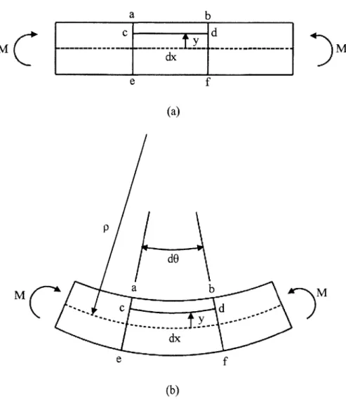
Fig. 2.1. B eam in pure bending ... 60

Fig. 2.2. Deformation of a beam in pure bending: (a) side view of beam, (b) deformed beam ... ... 61

Fig. 2.4. (a) Evolution of a beam through pure bending states, and

(b) Pure bending is independent of symmetric vertical motion ... 68

Fig. 2.5. (a) Initially straight beam with rigid clamps, (b) Deformed beam, and (c) H alf beam with sym m etry ... 71

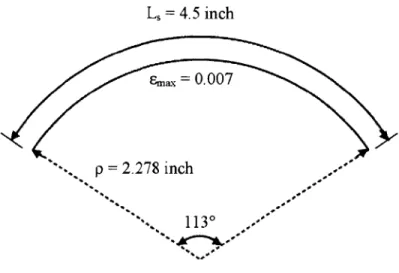
Fig. 2.6. Pure bending motion of beam ends for the example strand ... 75

Fig. 2.7. Beam deformed into a state of pure bending ... 76

Fig. 2.8. (a) Side view of circular-type bending mechanism, and (b) top view of circular-type bending mechanism ... 78

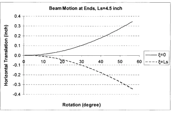
Fig. 2.9. Displacement at the beam end due to the lever arms ... 79

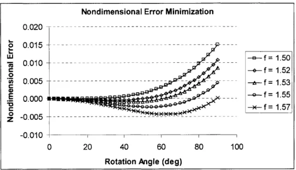
Fig. 2.10. Plot of nondimensional bending displacement error ... 83

Fig. 3.1. Drawing of the 195mm bore, 20T Bitter resistive magnet and cryostat at the National High Magnetic Field Laboratory (NHMFL) in Tallahassee, FL ... 86

Fig. 3.2. Bending mechansim (a) complete mechanism, (b) with strand mounting system removed, and (c) inner gear train ... 92

Fig. 3.3. Bending Mechanism Operation (a) 00 rotation angle, (b) 200 rotation angle, (c) 400 rotation angle, and (d) 700 rotation angle for the Torque Arms ... 94

Fig. 3.4. Strand Mounting System ... 95

Fig. 3.5. Support Beam Layout (a) Front View and (b) Back View ... 97

Fig. 3.6. Stress-strain curves for Ti6A14V annealed 0.064 inch sheet at various tem peratures ... . 99

Fig. 3.7. Support Beam and test strand distances from neutral axis to outer surfaces ... .... 100

Fig. 3.8. Current joint design with (a) All Components, and (b) Cut-Away View ... 104

Fig. 3.9. Strand Heat Treatment Fixture, (a) Fixture and Cap, (b) Main Fixture ... ... 106

Fig. 3.10. D etail of heat treatm ent fixture end ... 108

Fig. 3.11. Bending Mechanism ... 109

Fig. 3.12. Bending Mechanism Gear Train ... 111

F ig . 3 .13 . P rob e design ... 115

Fig. 3.14. Drawings of (a) cryostat, and (b) probe. All dimensions are in inches ... 116

Fig. 4.2. Sample mounting assembly for OST (Eurpean) strand withf= 1.53 ... 122

Fig. 4.3. (a) Current Joint mounting configuration, and (b) sample current-joint groove ... 123

Fig. 4.4. Position of sample in Support Beam ... 125

Fig. 4.5. (a) Sample side of the Support Beam, and (b) end of Support Beam showing compensating grooves ... 126

Fig. 4.6. Room temperature test of bending mechanism ... 133

Fig. 4.7. Permanent deformation of Support Beam tested at room temperature ... 134

Fig. 4.8. Probe and cryostat for the liquid helium bending mechanism verification test ... 135

Fig. 4.9. Support Beam tested in liquid helium bath ... 136

Fig. 4.10. Cell 4 at the National High Magnetic Field Laboratory ... ... 137

Fig. 4.11. Screen shot of testing control computer ... 138

Fig. 4.12. B ending test probe ... 140

Fig. 4.13. Bending Mechanism and Sample Assembly attached to probe ... 141

Fig. 4.14. Flexible current lead w ires ... 142

Fig. 4.15. (a) Attachment points for current lead wires, and (b) attached current lead wires ... 143

Fig. 4.16. Probe mounted on magnet cryostat ... 144

Fig. 4.17. Transferring liquid helium to the cryostat via the probe ... 145

Fig. 4.18. Voltage-current plots for IGC 157 Sample #1 (a) 0.2% strain, and (b ) 0 .1% strain ... 150

Fig. 4.19. (a) Current data, and (b) n-values for IGC 157 Sample #1 ... 153

Fig. 4.20. (a) Current data, and (b) n-values for IGC 157 Sample #2 ... 154

Fig. 4.21. (a) Current data, and (b) n-values for IGC 157 Sample #3 ... 155

Fig. 4.22. (a) Current data, and (b) n-values for EU 153 Sample #1 ... 156

Fig. 4.23. (a) Current data, and (b) n-values for EU 153 Sample #2 ... 157

Fig. 4.24. (a) Current data, and (b) n-values for EU 153 Sample #3 ... 158

Fig. 4.25. Measured bending strain for (a) IGC 157, and (b) EU153 beams ... 162

Fig. 4.26. Bending strain error for (a) IGC157, and (b) EU153 beams ... 164

Fig. 4.27. Effect of Lorentz load on bending strain for (a) IGC 157, and (b ) E U 53 b eam s ... 166

Fig. 4.28. EUl 53 test samples (a) before testing, and (b) after testing ... 168

Fig. 4.29. Offset between beam neutral axis and strand centerline ... 170

Fig. 4.30. Conceptual method for adding tensile strains to bending strain ... 174

Fig. 4.31. Bearing surface of bending mechanism Input Shaft ... 179

Fig. A. 1. (a) Beam with uniform load and fixed supports, and (b) moment distribution ... 187

Fig. C.1. B ending m echanism m odel ... 195

Fig. C.2. Bending Mechanism Parts List ... 196

Fig. C.3. Bending Mechanism Bottom Plate, Part No. PBD-001-001 ... 197

Fig. C.4. Bending Mechanism Top Plate, Part No. PBD-001-002 ... 198

Fig. C.5. Torque Gear A, Part No. PBD-001-003 ... 199

Fig. C.6. Torque Gear B, Part No. PBD-001-004 ... 200

Fig. C.7. Drive Shaft, Part No. PBD-001-005 ... 201

Fig. C.8. Input Shaft, Part No. PBD-001 -006 ... 202

Fig. C.9. Torque Arm 153, Part No. PBD-001-007 ... 203

Fig. C.10. Torque Arm 157, Part No. PBD-001-008 ... 204

Fig. C. 11. Beam Clamp A, Part No. PBD-001-009 ... 205

Fig. C.12. Beam Clamp B, Part No. PBD-001-010 ... 206

Fig. C. 13. Beam Clamp C, Part No. PBD-001-01I ... 207

Fig. C. 14. Beam Clamp D, Part No. PBD-001-012 ... 208

Fig. C.15. Thrust Bearing, Part No. PBD-001-013 ... 209

Fig. C .16. Plate Spacer, PBD -001-014 ... 210

Fig. C.17. Shaft Coupler, Part No. PBD-001-015 ... 211

Fig. C.18. Support Beam 153, Part No. PBD-001-016 ... 212

Fig. C.19. Support Beam 157, Part No. PBD-001-017 ... 213

Fig. C.20. Probe model ... 214

F ig . C .2 1. P rob e p arts list ... 2 15 Fig. C.22. Flange Plate, Part No. PBD-002-001 ... 216

Fig. C.23. Large Probe Plate, Part No. PBD-002-002 ... 217

Fig. C.25. Lower Small Probe Plate, Part No. PBD-002-004 ... 219

Fig. D.1. Bending Mechanism ... 221

Fig. D.2. Bending mechanism gear train ... 222

Fig. D.3. Bottom Plate, Part No. PBD-001-001 ... 223

Fig. D.4. Top Plate, Part No. PBD-001-002 ... 224

Fig. D.5. Torque Gear A & B, Part No. PBD-001-003 & PBD-001-004 ... 225

Fig. D.6. Drive Shaft, Part No. PBD-001-005 ... 226

Fig. D.7. Input Shaft, Part No. PBD-001 -006 ... 226

Fig. D.8. Torque Arm 153, Part No. PBD-001-007 ... 227

Fig. D.9. Front View, Support Beam 157, Part No. PBD-001-017 ... 227

Fig. D.10. Back View, Support Beam 157, Part No. PBD-001-017 ... 228

Fig. D.11. Machining Support Beam 157 ... 228

Fig. D.12. Beam Clamp C, Part No. PBD-001-011 ... 229

Fig. D.13. Beam Clamp D, Part No. PBD-001-012 ... 229

Fig. D .14. T op portion of Probe ... 230

Fig. D .15. Probe prepared for testing ... 231

Fig. D.16. Flange Plate, Part No. PBD-002-001 ... 232

Fig. D. 17. Flange Insulating Plate, Part No. PBD-002-005 ... ... 232

Fig. D.18. Large Probe Plate, Part No. PBD-002-002 ... 233

Fig. D.19. Upper Small Probe Plate, Part No. PBD-002-003 ... 233

Fig. D.20. Lower Small Probe Plate, Part No. PBD-002-004 ... ... 234

Fig. D.21. Bending Mechanism Insulating Plate, Part No. PBD-002-011 ... 234

Fig. E. 1. Furnace for heat treating IGC samples ... 237

Fig. E.2. Furnace for heat treating OST samples ... 237

Fig. E.3. Sample heat treatment fixture made from Ti6A14V ... 238

Fig. E.4. Heat treatment fixture and cap coated with Graphokote to prevent sintering ... 238

Fig. E.5. Grooves machined in sample heat treatment fixture ... 238

Fig. E.6. Heat treatment fixture after removing from furnace ... 239

Fig. E.8. Samples are one continuous strand ... 240 Fig. E.9. Removing samples from fixture ... 240

Table 1.1 Timeline for Nb3Sn conductor development ... 31

Table 2.1 Summary of the example strand specifications ... 64

Table 3.1 Values for estimating Support Beam torque ... 102

Table 4.1 Bending mechanism shaft rotation/strain state for [1.53 ... 132

Table 4.2 Bending mechanism shaft rotation/strain state forf-1 .57 ... 132

Table 4.3 Tensile strain in an offset strand with applied bending strain ... 172

Table 4.4 Bending strain in an offset strand ... 173

Table 4.5 Strain distribution in offset strand ... ... 175

Table A. 1 Estimate of actual bending strain at center of beam ... 184

Table A.2 Derivative estimate of actual bending strain at center of beam ... 185

Table B. 1 Gear parameters for bending mechanism wormgears and worms ... 191

Table B.2 Spline parameters for bending mechanism components ... 193

Table F. 1 Test sample voltage tap separation distances (inches) ... 241

Table F.2 Test data for IGC 157, Sample #1 ... 242

Table F.3 Test data for IGC 157, Sample #2 ... 243

Table F.4 Test data for IGC 157, Sample #3 ... 243

Table F.5 Test data for EU 153, Sample #1 ... 244

Table F.6 Test data for EU 153, Sample #2 ... 245

a: minimum radius of superconductor filament A: cross-sectional area

a: angle subtended by circular arc b: beam thickness

B: magnetic field intensity C1: constant of integration

C2: constant of integration

C3: constant of integration

CICC: cable-in-conduit-conductor C,: specific heat of superconductor d: strand diameter

db: beam thickness

d,: strand diameter

de: differential elongation

dx: differential length de: differential angle

5: offset of strand from beam neutral axis E: elastic modulus

E: critical electric field level c: bending strain

CB: bending strain in strand when strand is offset from beam neutral axis

Ebeam: bending strain in support beam

8

strand: bending strain of strand

&t: strain in strand caused by thermal contraction ET: strain in strand caused by tensile load

f nondimensional ratio between L, and L,

G: shear modulus of elasticity GF: strain gage Gage Factor

y,: mass density of superconductor h: beam height

H,: critical magnetic field Hy: applied magnetic field

HTS: high temperature superconductor I: current

I: critical current

I: moment of inertia

ITER: International Thermonuclear Experimental Reactor J,: critical current density

J0o: critical current density at operating magnetic field intensity ic: strain gage bridge constant

f: length

t : critical length twist pitch t,: twist pitch

ld: deformed length of line L,: undeformed length of sample

Lstrand: length of strand after deformation

L,: distance between rotation axes in bending mechanism LTS: low temperature superconductor

M: moment

p,: magnetic permeability

n: total gear ratio of bending mechanism N: normal internal force

w:

p,: electrical resistivity

Pstrand: radius of curvature of strand T,: critical temperature

T0: operating temperature

0: angle of rotation of bending mechanism lever arms u: horizontal displacement

Uerror: error in the beam end displacement from ideal

Uideal: ideal displacement of beam ends for pure bending

Umech: displacement of beam ends produced by bending mechanism v: vertical displacement

V: internal shear

VE: strain gage bridge excitation voltage

bV: change in the strain gage measurement voltage

: local axial coordinate y: distance from neutral axis

Introduction

The superconducting compound niobium-tin (Nb₃Sn) is an important technological material for building high field superconducting magnets. The superconductive state of Nb3Sn is sensitive to the strain conditions of the material. A considerable amount of research has been invested in trying to understand and predict this strain-dependent behavior so that more advanced magnet designs may be realized.

This thesis describes the design and testing of a variable-strain bending mechanism which was used to measure the bending strain dependent critical-current of two different internal-tin Nb3Sn strands, manufactured by Intermagnetics General Corporation (IGC) and Oxford Superconductor Technologies (OST).

1.1 History

A material that is in a superconductive state has the two prominent characteristics of being able to conduct electrical current without resistance and, more importantly, expelling magnetic field

effect, is the underlying means for conduction of electrical current without resistance in a superconductor.

Superconductivity is a phenomenon that is common to many materials when placed under the appropriate conditions. Each material has specific critical values of temperature, T,, magnetic field, H,, and current density, J, which express the limits of the superconducting state. In addition, some materials, such as Nb3Sn, have a superconductive state that is particularly sensitive to the strain state, &. These values, representing the transition between the

superconductive and normal resistive states, are often referred to as critical values. Thus the critical values establish a three-dimensional surface (or four-dimensional surface of properties if sensitive to strain), such as that shown in figure 1.1 which the material must be held within to remain superconducting.

J

Critical Surface

Fig. 1.1. Critical superconductive surface.

Kamerlingh Onnes discovered superconductivity in 1911 soon after he had successfully liquefied Helium in 1908. His original discovery came as he was testing the resistance of mercury with temperature. As he lowered the temperature below the 4.15 K critical temperature for mercury, the resistance suddenly dropped to zero. Onnes soon found several other materials that exhibited superconductivity at low temperatures, such as lead and indium.

After having established the critical temperatures for several materials, Onnes went on to find that there was also a critical magnetic field and critical current density. Realizing the potential of superconductivity, he built a solenoid magnet in 1913 using lead wire. This magnet could not remain superconducting beyond its own self-generated magnetic field of 0.08 T, establishing that there was both a critical magnetic field and critical current limit to the material.

The materials that Kamerlingh Onnes and his contemporaries studied had very low critical values that appeared to diminish any potential of using them for large power applications. These substances, now known as Type I superconductors, were not able to transport any appreciable amount of electrical current in the presence of a low magnetic field. Type I materials only allow magnetic flux penetration within a thin layer at the surface of the material, as described by the London Theory which was introduced in 1935. It was the discovery of a lead-bismuth alloy Type II superconductor by de Haas and Voogd in 1930 that initiated the advancement of high power superconductor applications [1.1].

1.2 Type II Superconductors

Type II superconductors are a mixture of Type I superconducting material with a distribution of normal resistive regions. The local islands of resistive regions allow magnetic flux lines to penetrate through the mixture without destroying the overall superconductive state. If a transport current were applied to an ideal Type II superconductor in the presence of an external magnetic field, the resulting Lorentz force would cause the magnetic flux lines to move and redistribute across the material. This is illustrated by figure 1.2. The movement of the flux lines is dissipative and requires a voltage to sustain the transport current in the conductor, thus eliminating the superconductivity [1.2].

VOLTA GE

TRANSPORT EXTERNAL FIELDHe

CURRENT, _Jit

Fig. 1.2. Dissipative flux motion in a Type II superconductor [1.2].

The flux lines may be pinned in place and prevented from moving by the presence of defects in the lattice structure of a non-ideal Type II superconductor. Vortices of magnetic flux penetrate through the normal regions and are surrounded by shielding currents. This establishes a pinning force that keeps the flux from moving and has the effect of raising the upper critical field level of the material. Each vortex contains one flux quantum which are arranged in a triangular lattice pattern throughout the material to minimize the energy state. This effect is illustrated in the drawing in figure 1.3a [1.3] and by an actual picture of the flux lattice in figure 1.3b [1.4]. Depending on the size and type of pinning site, there may be more than one flux quantum pinned.

Magnetic Flux Lines Grair Bounda Pin Vortex Transport Current (a) ries --ned T -Current (b)

Fig. 1.3. (a) Flux penetration in a Type II superconductor, and (b) picture of actual flux lattice [1.3,1.4].

The pinning sites of a Type II superconductor may be made up from several different types of imperfections in the bulk material including elemental inclusions, slip planes and other lattice defects, grain boundaries, and even voids from cold-working the material. The magnitude of the flux pinning force density depends on the type of pinning site and the superconducting material. Due to their differing pinning sites some Type II materials have higher flux pinning force density that others, as shown in figure 1.4 [1.5]. A higher flux pinning force density is desirable because

it results in a higher critical field level for the material.

Bulk

Pinning Force Comparison

10UMr T Ift- T MC *mid t7u%Wr wih nd.% 'ipm ;2duwn

4-'I Ii. 4a NbSn YBCO 4-~ - -a--NbN!AfN BM2

- -- e- I:N: 13nm-4M2nMi IMANMtRayr B.Gray at aL (AL) Physic C. 132' =

-E-

IWZVsO:lWR.

Nb-Ti

-+- 191iamWttap* BNlip. bt -Okada et al PUlachi

--- Hi2223: Roled 15 Fil Tpe(AwsC) B. UW6M -- .... -..-- Mg,'. M y mn" 3. Eam et at(W) u e 2002

-a-- Lf,: 10%wt SiC daped(Dou et al APL 2002.UW MgB₂

0 5 10 15 20 25

Applied Field (T)

hkbVn! W MW-CMO byPibr d I *-fp.Mp.marLt

Fig. 1.4. Flux pinning force comparison [1.5].

The concentration of pinning sites is just as important as the flux pinning force density in setting the critical field of a bulk Type II superconductor. Up to a point, increasing the number of flux pinning sites will allow more magnetic flux lines to penetrate the material and increase the

critical field level. The magnetic field will penetrate through the normal regions until these sites are all filled, at which point the flux must go through the superconductive regions. This quickly causes a breakdown in the superconductive state and marks the critical field level. When more normal pinning sites are available, a higher intensity magnetic field can be applied to the bulk material before the flux lines must move to the superconducting region. However, as the amount

n.m*Wa1 dimO -kamuw et it fIWASq

--- -lai: Mmmnd ibomn.s BEibbau..aliet ii. (UW-ASC) -aW-U- b: Bat Heat Teated UW Manvflianmt. (Li and

LaubalmsMe. IT)

-e-- lbT:l-llb (2116)331 mno nedllsayer 15 4515 0 iNlcm. McCarmidp et t ie)

--*+ - lsi:sn pad Cu APC. MduW6WC. R. Zhou PWD

Thesi ("n'"1

- U - Sa Sn Pled CUAPC2OOru@630C. hou at aLfOST).

- U -flb 3E: MlatbishTER MW hiwnal Sn

- lSa SnWand: Wih J, ermi Sn MW(Pen et al ASC~-M

Q4- l"/: Transfwnmd rod-40-be lb/i tachi.1M4M. lb Slammed. APL. vol. 71(1). pp-122-124). 1357

of resistive regions is increased it leave less available superconductive region for conduction of the transport current, thus reducing the current capacity of the bulk material.

The concentration and type of pinning sites throughout the bulk superconductor are dictated by the material constituents and fabrication processes. The combination of cold-work on the material and special heat treatments can be used to control the quality and quantity of pinning sites, thus improving the critical field and current density limits of the bulk superconductor. Much research goes into developing these processes to create a conductor with the best possible final properties for the given design.

1.2.1 Theories of Superconductivity

There are three significant theories of superconductivity that will be mentioned because of their importance to the subject, but will not be discussed in detail. These include the London Theory, the Bean and Anderson-Kim critical state models, and the BCS (Bardeen, Cooper, and

Schrieffer) Theory.

The London theory (1935) is a phenomenological theory that was a modification of Maxwell's electromagnetic theory to describe the Meissner effect (discovered in 1934). This theory establishes that the bulk superconductor is shielded from an external magnetic field by a supercurrent that flows in a thin layer at the surface of the superconductor and has a thickness equal to the London penetration depth, X.

The Bean model (1962) and Anderson-Kim critical state model (1963) establish the balance between the flux pinning force and the Lorentz force. The Bean model assumes that the critical current of the superconductor, J,, is a constant while Kim proposed that J, is proportional to the inverse of the magnetic field intensity, 1/B. These theories provide ways to estimate the magnetic field and current profiles within a superconductor and predict the magnetization curve of the material.

The BCS theory (1957) is a quantum mechanical theory that successfully modeled Type I superconductivity properties. It is based upon the concept that electrons close to the Fermi level form into Cooper pairs caused by an attraction related to lattice vibrations at the appropriate temperature and mediated by phonon interaction. The electron pairs are bosons that can behave very different from single electrons that must obey the Pauli Exclusion Principle. These pairs have a slightly lower energy level and leave an energy band of around 0.001 eV. This energy gap allows the pairs to avoid the collision interactions that lead to resistivity.

1.3 Superconductor Development

Applications of superconductors range from devices that simply exploit their behavior such as Josephson junctions to devices that place high demands on the superconductor, such as fusion reactor magnets. Of the thousands of superconducting materials that have been discovered there are only a few which are able to meet the demands of high field magnet applications. The environments in such magnets place the extremes of high field, high strain, high current, temperature instabilities, and sometimes radiation exposure on a superconductor.

At present, there are only three superconductors that have been used successfully in such extreme applications and include the two Low Temperature Superconductors (LTS) Nb-Ti and Nb3Sn and one High Temperature Superconductor (HTS) BSCC02223. There are four others that are under present development and which may be used in the future: Nb3Al and MgB2 as LTS and BSCCO2212 and YBCO for HTS [1.6].

Generally, it takes many years from the discovery of a superconducting material to its final development as a magnet-grade conductor. A timeline for Nb3Sn is given in table 1.1 and reveals that there was almost 30 years from the discovery of the superconducting properties of the material to the realization of a magnetic-grade conductor. Of, course as techniques become refined and the various problems worked out, the development process can be much faster for

subsequent materials. The development time to a magnet-grade Nb3Sn conductor was

particularly long because of various problems related to stability and coupling losses which had to be solved.

Table 1.1. Timeline for Nb3Sn conductor development [1.7].

The two most important problems that impeded early conductor development progress were flux jumping and coupling losses. The simple solutions turned out to be creating small

multi-filamentary strands with stability protection and twisting these filaments to minimize the area available for self-induced current. But it was only after much effort that these solutions were realized.

Flux jumping is an event when the magnetic flux within a superconductor is suddenly

rearranged. Under normal operating conditions the superconductor is in a stable state where the Lorentz force on the magnetic flux is just balanced by the pinning force. If some disturbance occurs to locally heat the superconductor then the critical current, J,, in that region will go down with the increase in temperature and flux motion will occur. Flux motion is dissipative and generates even more heat, which continues to locally raise the temperature. If the heating instabilities are not mediated by some means of protection then the positive feedback process

Stage Event Period

1 Discovery Early 1950s

2 Improvement Jc Early 1960s

3 Co-processing with matrix metal Mid 1960s

4 Multifilament/twisting, Ic>100 A Early 1970s

5 Long length, typically -1 km Mid 1970s

could quickly cause the material to transition into a normal conductive state and the subsequent Ohmic heating could permanently damage the conductor.

Most low temperature superconductors (LTS) have critical temperatures below 20K. Since the specific heats of materials are very small at these temperatures, it only takes a minor disturbance to raise the temperature of the material by several degrees. Disturbances that might cause a local temperature rise include a mechanical motion that generates heat by friction or a transient

magnetic field that causes an increase in current.

Being faced with this stability problem, early conductor designs were unsuccessful because the sources of the problem were not well understood. But over time adiabatic and dynamic

stabilization methods were developed which lead to practical conductors.

Adiabatic stability is achieved when the energy generated by Joule heating is balanced by the heat capacity of the superconductor material. An analysis based on the Bean model, Faraday's law, and the thermodynamic heat capacity of the material produces equation 1.1, which gives the minimum radius of the superconductor, a, for adiabatic stability. This expression requires the specific heat of the superconductor, Cs, the mass density, y, the magnetic permeability, p,,,, the critical temperature, Tc, the critical current density, J,,, at the operating magnetic field level, and the operating temperature, T0 [1.8].

Ta T 'I _(C.

p-j Jo

Using example values of

T, = 4.2K, Y,= 6.2 x IO3_kg/m3_,

B = 5T, C, = 1J/kg-K,

the minimum superconductor radius for adiabatic stability is a 68pm, or a diameter of d 140ptm. At low field levels J,, increases and J, is not a constant as assumed by the Bean model, but is a function of B. So, a conservative estimate of the superconductor filament

diameter for complete adiabatic stability is d 70pm. Present designs of superconducting strands have filament diameters as small as 3pm.

Dynamic stability is when the superconductive filaments are surrounded by a resistive material, such as copper, that has good thermal and electrical conductivity. Good thermal properties allow the heat generated in the superconductor to be quickly conducted away; good electrical

conductivity provides a pathway for the current to flow when the superconductor transitions into its highly resistive normal state. This additional material stops the heating progression by providing an alternate path for the current to flow and allowing the superconductor to cool back to its operating state.

Problems can occur within superconducting magnets that require active protection beyond stability methods. These problems include the breakdown of the insulation resulting in a short circuit between windings or large mechanical motions. Voltage sensors are placed at various points within the magnet to detect if a conductor begins to turn resistive, otherwise known as a quench. When this occurs the energy in the magnet can be quickly reduced by connecting a dump resistor across the magnet terminals or by switching on embedded heaters that heat the entire magnet above T,.

The discussion on stability has shown that the superconductor should be formed into small filaments and surrounded by a conductive metal matrix. Small filaments are limited by their critical current density and are not capable of transporting any significant amount of current, besides being difficult to handle. So in order to increase the current-carrying capacity and practicality, modem designs combine many superconductive filaments within a copper matrix to create what is known as a multifilamentary strand.

A strand is composed of many superconductive filaments electrically connected by copper or some other resistive stabilizer. The electrical connections between the filaments provided by the matrix allow the strand to experience coupling losses. A strand in the superconductive state has a current and magnetic field distribution through its interior that can be described by the Bean and Anderson-Kim critical state models. This distribution means that coupling occurs between adjacent filaments when an external magnetic field is applied. Starting with a fully coupled scenario, analysis can show that the amount of coupling can be reduced by twisting the filaments. Introducing a twist in the strand shortens the distance between points where the filaments cross, thus reducing the projected continuous area within the external field. For the strand to not be fully coupled, it must have a twist pitch below a critical length, i C , that can be calculated with equation 1.2. This equation uses the same definitions as in equation 1.1 with the addition of p, for the electrical resistivity of the matrix material in the strand and, Hy, for the applied magnetic field [1.9].

C = 16Jjap (1.2)

For a strand composed of superconducting filaments with a radius of a = 50Rm, a critical current

density of J,=3x1O9A/m2, a copper resistivity of pc=3xO10_{9i-m, and p}

0Hy = 0.01 T/s, the twist

pitch should be under t =27cm. For higher rates of expected field change, the critical twist pitch should be correspondingly smaller. As a general rule the twist pitch, t ,, is usually designed to be less than 10 to 15 times the strand diameter. So, for a 1mm diameter strand, the twist pitch should be t P 10-15mm.

It is important to note that although twisting is effective in uniform fields, it is only partially effective in non-uniform fields and completely ineffective with respect to self-fields. Self-field is the result of the transport current in the filaments and the filaments remain parallel to each

other regardless of any twist in the strand. This means that a large area is available for induced current to be generated by transients in the system.

1.4 Production of Nb3Sn Strand

The design and manufacture of magnet-grade conductors faces the practical problem of how to produce many twisted small filaments distributed through a stabilizing matrix within a single

strand. This discussion will be limited to a few of the methods for producing Nb3Sn-based strand because they are the most relevant to this thesis.

The Nb3Sn compound is a brittle material that cannot be drawn into lengths of strand using standard wire forming techniques. Methods have been developed to manufacture Nb3Sn strands by first combining together the necessary raw materials in a billet form and then passing the billet through a series of extrusion and annealing steps to achieve the desired strand diameter. The final step in forming the superconductor is a heat treatment that causes the constituents in the strand to react and form filaments of the Nb3Sn superconducting compound. Handling of the

strand after the Nb3Sn has been formed must be done with extreme care because the brittle material can fracture easily.

The ingredients combined in the raw billets include niobium and tin for the superconductor, copper for the matrix material, and a tantalum or niobium barrier to keep the tin from diffusing into the copper and forming lower-conductivity bronze during the heat treatment. These materials are combined using one of several different techniques and then drawn as a unit down to the final strand size. Each of the components has different material properties that make it

difficult to extrude them together, so various annealing steps are often included to help the process.

Copper is most often chosen as the matrix material because it is a highly ductile material that has excellent conductivity and combines well with the other materials. The ratio of

copper-to-superconductor in the strand is typically in the range of 1:1 or 2:1. This relationship has been shown to provide good stability while not occupying too much of the strand diameter available for current transport in the final product. Of course, different applications may use a strand with a slightly different amount of stabilizer.

There are six contemporary manufacturing methods for creating Nb3Sn strand: Bronze, Internal Tin, External Diffusion, Nb Tube and Sn Tube (Powder-in-Tube, PIT), Jelly Roll & Modified Jelly Roll, and Cable-in-Tube (CIT). Only the first three methods will be covered because they

are the most relevant.

Bronze process starts with a bronze billet that is drilled with a pattern of holes which are filled with niobium as shown in figure 1.5a. Several of these billets are extruded into hexagonal shapes and then stacked into a copper can with an interior tantalum barrier. The can is sealed and evacuated and then extruded followed by drawning into the final strand diameter as

illustrated by the process outline in figure 1.5b [1.10]. This extrusion process is similar for many of the multifilament strand techniques.

Extrude into ₀₀ Hexagonal Shape Cu-Sn Nb

0

0 0

0

0

FCold

[~Draw

Fig. 1.5. (a) Bronze billet pattern, and (b) Multifilament drawing process [1.10]. Seal & Evacuate

Preheat & Extrude

A picture of a Bronze process strand cross section is shown in figure 1.6. The view of the entire cross-section reveals the light outer copper surface with the darker tantalum barrier surrounding the filament pattern. The magnified view shows the individual filaments and the hexagonal pattern.

Fig. 1.6. Picture of bronze process strand [1.11].

Internal Tin process begins with a pure copper billet that is drilled and filled with niobium and tin in a pattern similar to figure 1.7a. These billets are combined and drawn together to form a single strand. The extrusion and annealing steps are different than with the Bronze process because the constituents have different material properties. The barrier is usually co-extruded with the surrounding copper stabilizer. The Nb-Cu-Sn subelements are then restacked inside the barrier tube and drawn to final wire size. The picture of the internal tin strand cross-section in figure 1.7b shows that the tin core occupies a significant portion of the area. The tin must diffuse through the copper surrounding the niobium filaments and combine to form the Nb3Sn

compound during the heat treatment. This ends up creating a bronze matrix because tin has a greater affinity for copper than niobium. The outer copper shell and the tantalum barrier that keeps the tin from diffusing to the surface are clearly visible in the picture. The Internal Tin

- Cu

Nb

-q~~Sn PO

(a) (b)

Fig. 1.7. (a) Internal Tin billet, and (b) Picture of unreacted Internal Tin strand [1.12].

External Tin process is similar to Internal Tin in that it relies on the transport of tin through the copper to react with the niobium during heat treatment. However, the tin is added to the surface after the copper billet has been filled with niobium rods and extruded. The extrusion is plated with tin and then combined with similar extrusions which are drawn together to form the strand. Figure 1.8 shows the general layout of the external diffusion billet after it has been plated with tin. This process is not often used because it either requires too fine subelements or results in too small of a wire diameter.

Nb

Cu

A

S

Other strand processes are based upon the same concept of bringing the materials together and forming a strand that is later heat treated to produce the Nb3Sn compound. The primary differences are in the configuration and steps used to create the strand. Some of the processes result in a strand with a higher J,, while others produce an advantage with respect to AC losses. The cold working and annealing steps are carefully adjusted for each process so that either the J, is maximized or the AC losses are minimized after the final heat treatment.

During heat treatment, the niobium and tin can diffuse and create bridges connecting filaments together. This is detrimental to the strand performance because the coalescence of the filaments creates a much larger effective diameter which, as was shown earlier, increases the likelihood of flux jumping as well as higher magnetization losses.

TvistAnneal

Spool Test Plating

(optional)

After the strand has been drawn to its final size it is twisted to a specified twist pitch in order to reduce coupling losses. The general twisting steps are similar for the different strand designs and are shown in figure 1.9. The strand may be plated with chrome to give it a protective surface which eliminates strand-to-strand diffusion bonding during heat treatment. This is used when the strands are cabled together to form a large conductor.

1.5 Cable-in-Conduit Conductor (CICC)

After the strand has been produced it is assembled into a conductor configuration for use in the windings of the magnet. Different types of magnets use different conductors based on the design requirements. Depending on the conductor design, the superconducting strand is maintained below its critical temperature using either conduction or the flow of a cryogen fluid. The magnet windings may be in a bath of cryogen as in MRI and NMR machines or have a cryogen flow forced through the conductor as in fusion magnets and high-energy physics dipoles and quadrupoles. Liquid-free conduction-cooled magnets are emerging in a wide variety of applications mostly because of improvements to cryocooler performance.

Superconducting magnet conductors are generally composed of the superconductor, an electrically conductive material for stability (Cu, Al, or Ag), the cooling system, and a high-strength metal for structural support [1. 15]. A magnet conductor design should be able to transport the maximum current density while providing electrical insulation, cooling, stability,

and mechanical integrity all at the lowest possible cost.

The cable-in-conduit conductor (CICC) is composed of a cabled superconductor in a metal conduit cooled by forced-flow supercritical helium. Its current carrying capacity combined with its stability protection and inherent mechanical strength make it suitable for applications that use high field, large volume magnets, such as in ITER (International Thermonuclear Experimental

Reactor) [1.16]. CICC was originally conceived circa 1975 and has subsequently received much development attention. [1.17].

A picture of a disassembled length of CICC designed for use in the ITER CSMC (Central

Solenoid Model Coil) is shown in figure 1.10 [1.18]. This conductor is made up of a

combination of Nb3Sn internal tin superconducting strands and copper wires used for quench protection which are twisted together in several stages to create the final cable. The twist pattern for this cable can be seen in the figure and shows that groups of three strands are first twisted together and then combined in subsequent twist stages to form the cable structure. Each stage has a specified twist pitch and the overall pattem can be described by a series that represent the number of groups twisted together at each stage; for this CICC it is 3-3-4-5-6 = 1080.

A cross-sectional view of a CICC in figure 1.11 shows some of the additional features of the conductor [1.19]. The six final petals of the cabling are oriented around a stainless steel spring that maintains a central cooling channel for the single phase supercritical helium flow. The

helium fills the void space and conducts away excess heat as it is forced through the magnet windings. Long lengths of cable are inserted into welded extrusions of a nickel-steel superalloy conduit of Incoloy Alloy 908 which is compacted around the cable to the final dimension.

A series of magnifications of the conductor in figure 1.11 show the cross-section of a single strand followed by a small group of the over 1100 filaments in the internal tin configuration and concludes with a micrograph of one of the 3pm diameter Nb3Sn filaments. After assembling the CICC it must be heat treated to form the Nb3Sn superconducting compound. The reaction may occur either before or after the conductor assembly has been formed into the magnet windings, depending on the design procedure. In the case of ITER, the conductors are formed into the magnet windings before the reaction heat treatment to form the Nb3Sn phase.

One of the primary applications for the cable-in-conduit conductor is in large fusion reactor magnets such as those intended for ITER. Figure 1.12 is a picture of a computer model of the ITER design showing the relative scale along with the various magnets and systems [1.20]. The six central solenoids that are used to heat the plasma are at the core of the reactor and the toroidal field coils used to contain the plasma can be identified by their characteristic D-shape. Poloidal field coils surrounding the containment chamber at different elevations are used to shape the plasma.

Fig. 1.12. Computer model of ITER (International Thermonuclear Experimental Reactor) [1.20].

ITER is an experimental reactor that is a step between contemporary fusion reactors used to study plasma and future reactors that will be capable of generating electricity. It is an international project involving The People's Republic of China, the European Union and

the United States of Amenica. It is planned to be built in Cadarache, near Aix-en-Provence, France and is technically ready for construction to begin. The first plasma operation is expected to take place in 2016 [1.20].

Within fusion magnets, such as those found in ITER, large electromagnetic Lorentz forces are generated which place tremendous loads on the components. In particular, the brittle Nb3Sn

strands which make up the conductor experience a complicated combination of mechanical stresses. It is important to understand the effect of these loads on the strain-sensitive strand in order to design reliable magnets that will operate at their expected levels.

As described before, the strands are twisted in several stages into cables and then compressed into the structural jacket. This combination of cabling and compression means that the pathway of a single strand through the conductor is complicated and irregular. The strand may be

positioned next to the jacket wall at one point and then migrate to the inner channel at a different axial distance along the conductor; it can run parallel to neighboring strands or cross over them causing a potential pinch point.

When the conductor is carrying current in a large magnetic field the pathway followed by the strands leads to a complicated evolution of tension, compression, bending, and pinching strains as the Lorentz forces are applied. The effect of the Lorentz force accumulates within the conductor because, in addition to having their own electromagnetic forces, the strands closer to the magnet axis push against those strands further from the axis. These resulting strains can

significantly degrade the ability of the Nb3Sn superconductor to transport current. Much work has gone into trying to understand the strain-related behavior of Nb3Sn not just for fusion magnets but for any application that places a strain-sensitive superconductor under a load.

1.6 Strain Behavior of Nb3Sn

The strain-related behavior of Nb3Sn was studied by Buehler and Levinstein approximately a decade after its identification as a superconductor [1.21] and it was almost 20 years later that Ekin presented a strain scaling law that could be used for the design of practical superconductors [1.22]. This early work was primarily concerned with the uniaxial tensile and compressive effects on the current capacity of Nb3Sn with some thought given to bending strain effects [1.23]. The research showed that the application of tensile strain first increased the critical current capacity of Nb3Sn strand up to point before it began to decrease. This was explained by a pre-compression on the Nb3Sn that was applied by the surrounding matrix materials due to the different coefficients of thermal expansion as the strand was cooled from the reaction temperature to the operating temperature.

Since those pioneering studies, substantial work has gone into better understanding the strain behavior of Nb3Sn strand and developing improved strain scaling laws that are used for magnet design. A general overview will be given of the various efforts that have been undertaken to understand the strain behavior of Nb3Sn. Rather than focusing on a single type of strain

research, this overview will present a variety of studies that will serve to illustrate the numerous issues that surround the problem. The amount of effort that has gone into understanding the strain behavior of Nb3Sn and other superconducting materials is an indication of the importance of this problem to superconductor applications. This effort has been driven by the need for better design tools as the boundaries of experience are pushed by new and more demanding magnet requirements.

1.6.1 Uniaxial Strain

The material surrounding the Nb3Sn filaments in a strand places an intrinsic compressive strain on the superconductor upon cool-down. The exact value of this compressive strain depends on the particular arrangement and quantities of the several materials in a given strand design, but typically is around -0.3% strain. Application of an external tensile axial strain to a strand

relieves this compression and increases the critical current. If the applied strain goes beyond this amount, then the critical current begins to degrade. Appling a compressive strain on a Nb3Sn sample will just serve to degrade the critical current level from the intrinsic cool-down state.

Figure 1.13 shows a plot of the critical current in a Nb3Sn strand as a function of an applied tensile strain. The strand characterized in the plot was produced by Teledyne (TWC) and used in the 45T Hybrid magnet at the National High Magnetic Field Laboratory (NHMFL) [1.24]. The figure reveals the increase and subsequent degradation in the critical current of the strand as the applied strain goes to +0.3% and beyond. The open points are I measurements during loading and the closed points are measurements after unloading. The unloading began at the point marked "A" and measurements were done at 4.2K in a background field of 12T perpendicular to the sample.

40 0

S0-o

Strain, %

Fig. 1.13. Strain dependent critical current in the 45T Hybrid magnet strand at 12T and 4.2K [1.24].

A common practice when reporting strand strain behavior measurements is to move the data so that it is in terms of the intrinsic strain on the filaments. This consists of normalizing the critical current to the maximum value and shifting the data so that the new zero-strain point corresponds to this peak current. Figure 1.14 shows such a plot for an internal tin 00.8mm Nb3Sn strand manufactured by Oxford Superconductor Technology (OST). An adjusted intrinsic strain of 0.0% results in the maximum measured current for the sample at external field levels of 17T,

19T, and 20T. The critical current value was defined for an electric field of 0.1 pV/cm, which will be explained in detail in chapter 4. The dashed lines represent fitting of the data to the strain scaling model developed by Ekin for predicting strain dependent behavior. Strain was applied to the sample using a popular device known as a Walters Spring (WASP) [1.25].

1. 0. 0. 0. 0. 0. 0. 0. 0. 0. 00 9. 63 WI _ _ _20-- 3-21T _{Nb n -I rnal}

_In

Fig. 1.14. Reduced critical current vs. intrinsic strain for OST internal tin wire [1.25]. o

Uniaxial strain tests of Nb3Sn are often performed with mechanisms that are capable of loading the sample through a large range of tension and compression in order to get a more complete

understanding of the strand behavior. The mechanisms are designed to be used in the bore of a magnet that can produce a field intense enough to measure the critical current of the sample over a useful range. Requiring the test to take place in a magnet bore severely limits the length of the sample, which is unfortunate because longer samples give more sensitive measurement results. There are three devices that are prominent in studying the strain-behavior of technological superconductors: a U-spring holder, a device known as "Pacman", and the Walters Spring.

The U-spring device has been used in various forms over the years to apply strain to superconducting samples. An example of one used at the University of Twente is shown in figure 1.15 [1.26]. The sample is mounted across a bridge that is either stretched or compressed by movement of the device's legs. It is a versatile and reliable system for characterizing the strain behavior of technical superconductors, but it has limitations with respect to the length of the sample that can be measured. Consequently, other devices intended to lengthen the sample have been developed.

--- Tbermoseter 45n -- Strain dpsk _{_} -- -- -- -- _{S a p} l e h o l e r .-- --- -Tape smupe---5 nun L Tape --< 0 Strain p.p e--- -0 Struin pop

HM---Strain adjustmunI Cnue%-uetloon (top)

The Pacman device shown in figure 1.16 was developed at the University of Twente. This mechanism lengthens the sample from the -45mm of the U-spring to -104mm. Of course, the effective test measurement distance is shorter than this, but it has resulted in a factor of 10 increase in length. The sample is affixed to the outside diameter of the holder and when a pure torque is applied to the ends of the circular beam section the beam diameter changes. This results in either a tension or compression in the test sample. Aside from the end effects, analysis

shows that the strain in the test section is fairly uniform and introduces little bending [1.26,1.27].

2 I

3

-7 e36

3 2.53 000

5

Fig. 1.16. Pacman strain device used at the University of Twente [1.26,1.27].

The Walters Spring (WASP) is an ingenious mechanism presented in 1986 that significantly increases the sample length for strain measurements [1.28]. The Walters Spring has been adopted and modified for use by several researchers to study the strain behavior of both Low Temperature (LTS) and High Temperature Superconductors (HTS) [1.29,1.30]. Figure 1.17

shows the device used by Institute of Applied Physics at the University of Geneve, Switzerland [1.25,1.31,1.32].

This WASP device can hold a sample length of 80cm and the Ti6Al4V spring alloy allows linear and reversible strains up to 1.4% to be applied at 4.2K. The sample is wrapped around the outer surface of the spring and either lies in a groove or is fixed by soldering. The mechanism

operates by applying opposing torques at each end of the spring. It has benefited from many years of refinement and is one of the more common devices used for characterizing the strain-behavior of Nb3Sn strand.

mnt contaot

stram gauge Ti alloy spring Nb3Sn wire

Fig. 1.17. The Walters Spring (WASP) device for measuring critical current as a function of strain [1.31].

The critical current information collected from the various strain methods is intended to improve understanding of the behavior of strain-sensitive superconductors. This data is then used to develop and improve universal strain scaling laws for use in magnet design. Being able to

accurately predict the performance of the superconductor within a magnet allows designs to be created that optimize the use of the expensive superconducting materials.

1.6.2 Strain Scaling Laws

Scaling laws have been developed to predict the behavior of technological superconductors in a practical design. Those superconductors with little or no strain sensitivity have relationships that

express the behavior of the material in the three-dimensional space of current density, temperature, and magnetic field. But those superconductors with strain-sensitivity, such as Nb3Sn, have a slightly more complicated description that includes additional parameters to

account for the strain effects.

Superconducting magnet designs have often avoided the added cost and uncertainty associated with using a strain-sensitive superconductor by using less strain dependent materials, such as NbTi. This limited the potential capability of those magnets because the strain-sensitive superconductors, such as Nb3Sn, have inherent critical properties that allow them to produce higher magnetic field levels. The maturation of strain scaling laws provided a means for more

accurate designs to be created using these materials as the need for magnet performance intensified.

In 1980, Ekin presented a universal strain scaling law for practical superconductors [1.22]. This law and its refinements have been particularly successful for Nb3Sn conductors and has allowed many magnets to achieve their design parameters. The Ekin scaling law was expanded to include temperature dependence and the effects of nuclear radiation by Summers in 1991 [1.33]. Work on the development and refinement of universal scaling laws continues to be done in an

effort to extend the range and accuracy of these predictive tools [1.34,1.35,1.36].

The Summers-Ekin scaling law for Nb3Sn is presently the most common method for designing magnets. Expressions for this scaling are given by equations 1.3 to 1.11. This scaling law consists of a few simple expressions for the critical current density, J", and the critical temperature, T,, which are modified by additional expressions that compensate for the strain