Amplitude and frequency demodulation controller for MEMS accelerometer

Amplitude and Frequency Demodulation

Controller for MEMS Accelerometer

by

Lane Gearle Brooks

Submitted to the Department of Electrical Engineering and Computer

Science

in partial fulfillment of the requirements for the degrees of

Bachelor of Science

and

Master of Engineering in Computer Science and Engineering

at the

MASSACHUSETTS INSTITUTE OF TECHNOLOGY

February 2001

@

Lane Gearle Brooks, MMI. All rights reserved.

The author hereby grants to MIT permission to reproduce and

distribute publicly paper and electronic copies of this thesis document

in whole or in part.

''0

Author ...

BARKER

Department of Electrical Engineering and Computer Science

December 15, 2000

Certified by...

...

Paul Ward

Charles Stark Draper Laboratory

I

Certified by...

Accepted by..

,Thesis

Rahul Sarpeshkar

*sAdt

ifsor

krthur C. Smith

Chairman, Department Committee on Graduate Students

1MASSACHSMlS

INSTITUTE-OF TECHNOLOGY

JUL 11 200

Amplitude and Frequency Demodulation Controller for

MEMS Accelerometer

by

Lane Gearle Brooks

Submitted to the Department of Electrical Engineering and Computer Science on December 15, 2000, in partial fulfillment of the

requirements for the degrees of Bachelor of Science

and

Master of Engineering in Computer Science and Engineering

Abstract

Draper Laboratory is developing a high precision MEMS accelerometer. This thesis describes and analyzes the electronics which produce the acceleration estimate and control the actuators within the sensor. The Vector Readout method of amplitude and frequency demodulation is described and shown to be a high precision, environmen-tally stable method of demodulation. The Vector Readout method of demodulation uses a Hilbert Transform filter and the CORDIC algorithm to simultaneously esti-mate both the amplitude and phase of a signal. A feedback controller is designed to hold the oscillation of a mass resonator at a constant amplitude.

Thesis Supervisor: Paul Ward

Title: Charles Stark Draper Laboratory Thesis Advisor: Rahul Sarpeshkar Title: Assistant Professor

Acknowledgments

The thesis was prepared at The Charles Stark Draper Laboratory, Inc., under Draper Laboratory IR&D project 13066. Publication of this thesis does not constitute ap-proval by Draper or the sponsoring agency of the findings or conclusions contained herein. It is published for the exchange and stimulation of ideas.

Author

Lane Brooks

I must thank many people who have helped me to get to this point. There are the obvious people of my parents, wife, family, and teachers. There are also several people that I must specifically acknowledge in helping me with this project:

Paul Ward: Paul is my advisor at Draper Laboratory, and he has generously given of

his time in discussions with me. It is through these discussions and his written documents that I learned a lot of this material. He and others had been thinking about this project well before I started it, and they really laid the foundation of it.

Dave McGorty: I worked with Dave in implementing this project. His digital logic

im-plementation experience greatly helped me. Furthermore, he helped to develop the demodulation method used for this project.

Rich Elliott, Marc Weinberg: I worked for Rich and Marc for two summers testing MEMS gyros prior to working on this thesis. It is their time and efforts with me that

enabled me to understand much of the physics and control issues with this project. Rahul Sarpeshkar: Professor Sarpeshkar and others in his group provided very useful

feedback on this project. His probing questions really forced me to think about alternatives and subtleties. Furthermore, Professor Sarpeshkar was my recitation instructor who taught me almost everything I know about classical control, so he is the one who enabled me to figure out and write Chapter 6 of this thesis.

Other Draper Employees: Tom King, Amy Duwel, Nathan St. Michael, Brian Johann-son, Judy Nettles all helped me out in various ways with this project.

Contents

2 Vector Readout Method of Demodulation 21 2.1 Vector Readout Overview . . . . 21

2.2 A/D Converter . . . . 23

2.3 Quadrature Generation Via Hilbert Transform . . . . 24

2.3.1 Ideal Hilbert Transform Filter . . . . 24

2.3.2 FIR Hilbert Transform Filter . . . . 26

2.4 CORDIC Algorithm . . . . 28

2.5 Implementation Details . . . . 32

3 Frequency Demodulation Analysis 35 3.1 Noise Source Definitions and Metrics . . . . 35

3.2 Vector Readout FM Demodulation Analysis . . . . 38

3.2.1 Intrinsic Noise of Vector Readout Method . . . . 39

3.2.2 Input Noise Sensitivity . . . . 50

3.3 FM Demodulation Comparison . . . . 52

4 Mapping Frequency To Acceleration 57

4.1 Compensation Methods . . . . 57

4.1.1 First Order Compensators . . . . 60

4.1.2 Spring Stiffness Variation . . . . 63

4.1.3 Sampling Clock Drift . . . . 65

4.1.4 :Noisy Frequency Estimates . . . . 65

4.1.5 Compensation Method Selection . . . . 73

4.1.6 Parameter Selection . . . . 73

5 Amplitude Demodulation Analysis 75 5.1 Noise Source Definitions . . . . 75

5.2 Vector Readout AM Demodulation Analysis . . . . 76

5.2.1 Intrinsic N oise . . . . 77 5.2.2 Input N oise . . . . 78 5.2.3 Sum m ary . . . . 79 5.3 AM Demodulation Comparison . . . . 80 5.3.1 Conclusion . . . . 81 6 Controller Design 6.1 Amplitude Disturbances . . . . 6.2 Sensitivity of Acceleration Measurement To Amplitude . . . 6.3 Controller Overview . . . . 6.4 Amplitude Control . . . . 6.4.1 The Amplitude Transfer Function of the Plant . . . . 6.4.2 The Transfer Function of the Demodulator . . . . 6.4.3 Defining Nominal System Parameters . . . . 6.4.4 Designing The Controller . . . . 6.4.5 Designing Around the Open Loop Transfer Function 6.4.6 Stability M argins . . . . 6.5 Conclusion . . . . 83 83 85 . . . . 87 . . . . 89 . . . . 89 . . . . 93 . . . . 94 . . . . 95 . . . . 106 . . . . 108 . . . . 109

7 Conclusion 111

7.1 Design Specification Check . . . .111

7.1.1 Dynamic Range (1pg to 100g) . . . .111

7.2 Implementation Details . . . . 113

7.3 Data Collection Software . . . . 117

7.4 Real Data . . . . 119

List of Figures

1-1 Accelerometer Input/Output Representation . . . . 17

1-2 Block Diagram of General Readout Tasks . . . . 18

1-3 Block Diagram of Readout & Controller Tasks . . . . 19

2-1 Vector Readout Method of AM and FM Demodulation. . . . . 22

2-2 In-Phase & Quadrature Signals Represented as a Complex Vector. . . 22

2-3 Implementation Block Diagram of Vector Readout Method. . . . . 23

2-4 Implementation of Hilbert Transform Filter and In-Phase Delay. . . . 28

2-5 Example of CORDIC Algorithm . . . . 31

3-1 The Ideal FM Demodulator Outputs the Instantaneous Frequency. . 35 3-2 Non-Ideal FM Demodulator Representation . . . . 36

3-3 Additive Input Noise Representation . . . . 36

3-4 Output Noise Representation . . . . 37

3-5 Block Diagram of Vector Readout Method of FM Demodulation. . . . 38

3-6 A/D Quantization Noise Represented as Additive Noise Source . . . . 39

3-7 Unit Sample and Frequency Response of Hilbert Transform Filter. . . 41

3-8 A/D & Hilbert Transformer Noise Representation . . . . 42

3-9 Ripple in Pass Band of Hilbert Transform Filter . . . . 43

3-10 Single Noise Source Representation . . . . 45

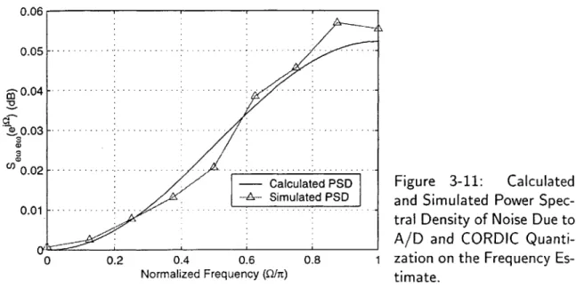
3-11 PSD of Frequency Estimate Noise . . . . 49

4-1 Different Compensation Methods . . . . 59

4-3 Acceleration Bias From Common and Differential Frequency Noise . 4-4 White Noise Random Walk . . . . 4-5 Differentiated White Noise Random Walk . . . .

5-1 The Ideal AM Demodulator Outputs the Instantaneous Amplitude. 5-2 Amplitude Demodulation Using Vector Readout method . . . . 5-3 Nature of Bias From Vector Readout AM Demodulation . . . . 6-1 _{Comparison of Approximated and Simulated Natural Frequency . .} 6-2 AGC Controller Block Diagram . . . . 6-3 Outer Loop Collapsed To A Variable Gain Block Labelled AGC. . .

6-4 Amplitude Controller Block Diagram Reduction . . . .

6-5 Controller With Amplitude Demodulation Dynamics Included . . .

6-6 Plant and AM Demodulation Transfer Function.

Amplitude Controller Block Diagram . . . . Control Loop With Additive Disturbance . . . . Amplitude Control Loop With Additive Noise . . . . Closed Loop Amplitude Demodulation Noise Response. . . .

First Order E-A Modulator. . . . .

D/A Conversion With E-A Modulator. . . . .

Quantization Noise From E-A D/A AGC Conversion. . . . . Block Diagram Depicting Additive E-A Quantization Noise.

E-zA Quantization Noise To Amplitude Transfer Function. .

Open Loop Transfer Function of System. . . . . Open Loop Transfer Function With

Q

96 . . . . . 97 . . . . . 99 .. ... 100 . . . . . 102 . ... 102 . . . . . 104 . . . . . 105 105 . . . . . 107 . . . . . 109 . . . . . 110

7-1 Data Collection Software . . . . 7-2 Data Collected From Accelerometer . . . . 118 119 68 70 72 75 76 80 86 88 88 90 93 . . . . 95 6-7 6-8 6-9 6-10 6-11 6-12 6-13 6-14 6-15 6-16 6-17 6-18

List of Tables

3.1 Summary of Intrinsic Noise Sources on the Downsampled Estimate of the Phase. ... ... 47

3.2 Summary of Frequency Estimation Errors Using Vector Readout Method for FM Demodulation. . . . . 53

4.1 Summary of Spring Stiffness Variation Results . . . . 64 4.2 Acceleration Bias Resulting From Sampling Clock Drift. . . . . 66

4.3 Comparison Acceleration Estimation Bias Under Different Compensa-tion m ethods . . . . 68

4.4 Variance and Velocity Random Walk From White Frequency Noise . 70

4.5 Variance and Velocity Random Walk From Differentiated White Noise 72 6.1 Nominal Values For Sensitivity of Accelerometer to Changes in

Ampli-tude. ... ... 87 6.2 Nominal Accelerometer System Values . . . . 94

7.1 Acceleration Estimation Bias Errors and Velocity Estimation Random W alk. . . . . 114

Chapter 1

Introduction

1.1

Project Overview

Draper Laboratory is working to build a high precision MEMS Vibratory Accelerom-eter (VA), and the project discussed in this thesis is part of that effort. The tasks of this thesis are to design, analyze, and implement two components of the system. One is the signal processing which produces the acceleration readout, and the other is the controller which controls the resonator within the accelerometer to ensure an accurate acceleration readout.

Project Objectives

Within the Vibratory Accelerometer is an oscillating mass whose spring stiffness changes as a function of the acceleration. This changing spring stiffness changes the resonant frequency of the oscillator-just as when one tunes a guitar string, the natural frequency of the string changes as the spring stiffness of the string changes. As a result, there are two specific tasks that the electronics of the accelerometer must perform.

Readout Objectives: One task is to generate a readout signal indicating the amount

of acceleration the device is experiencing. This is done by determining the in-stantaneous frequency of the output signal of the accelerometer and translating

that frequency into an acceleration estimate.

Controller Objectives: The second task is to generate a control signal to hold

the amplitude of the resonating mass constant. This is necessary to obtain an accurate readout measurement because the resonator has non-linearities which couple the amplitude and frequency.

Design Specifications

The accelerometer must meet very aggressive design specifications which are:

Dynamic Range: lpg to 100g Acceleration Error: < 1Ipg

Velocity Random Walk: < 0.014 ft

To ensure that the electronics can meet these constraints, the system will be analyzed under two conditions. The first is under the assumption that the resonator within the accelerometer is an ideal second order system. Then the intrinsic noise sources of the electronics can be characterized and analyzed to ensure that they can meet the specification. The second condition which will be analyzed is when various noise sources that model the imperfections of the system are injected into the signal path. This will ensure that the the electronics are designed well enough so that the system as a whole can meet the design specifications.

1.2

Sensor Details

For this project, the accelerometer can be represented as a block as shown in Figure

1-1*. One input, labeled f(t), is the force applied to the resonating mass within the sensor. This force keeps it oscillating. The other input signal, labeled g(t), is the acceleration that the device experiences, and it is the signal that we are trying to estimate for readout. The output signal, labeled x(t) in Figure 1-1, is a measurement

*For simplicity, only one oscillator is included in this discussion. In reality there is a second oscillator which produces a fully differential signal. The second oscillator is discussed only when it

g - VA x(t) Figure 1-1: Accelerometer Input/Output

f(t) Representation

of the position of a mass resonator within the sensor. Modeling the resonator as a second-order system, the position can be described by the differential equation

mt(t) + bi(t) + k(t)x(t) = f (t), (1.1)

where m is the mass, b is the viscous damping, and k(t) is the spring constant of the mass resonator. Notice that k(t) is not constant. It can be modeled as an affine functiont of g(t):

k(t) = k1 + kgg(t). (1.2)

1.2.1 Readout Details

The goal of this accelerometer is to obtain an estimate y(t) of the actual acceleration g(t) using the position signal x(t). The model of the position and acceleration signals as expressed in Equations 1.1 and 1.2 provides a the relationship between x(t) and g(t). However, since k(t) is not constant, solving Equation 1.1 for x(t) in a closed form is difficult if not impossible. Several books, such as Reference [6], have been devoted to techniques of finding approximations to the solution of Equation 1.1 in closed form under certain constraints. Ve will use some of these approximations later. Now, we make a simple approximation to the solution by realizing that when k(t) is constant and when the force being applied exactly cancels the damping (f(t) = b±(t)) that the

system will ring at its natural frequency, which is u; = . Thus if the controller is built to force the system to ring at its natural frequency, then the relation between the frequency of the position signal and the acceleration will be

k1 + kgg(t) (1.3)

wn(t) =.(.)

m

is applicable.

tSince the affine relationship dominates, higher order relations between k(t) and g(t) will be neglected.

This means that if the position signal x(t) is frequency demodulated to find the instantaneous operating frequency of the resonator, we will have obtained an estimate &n(t) of the actual natural frequency w,(t). Since it is possible to invert Equation 1.3, the acceleration can then be estimated as

(t) = + (1.4)

Therefore, we have a means of estimating the acceleration g(t) by frequency de-modulating the position signal x(t) and then performing the nonlinear compensation described in Equation 1.4. This is shown in the block diagram in Figure 1-2.

g(t) x(t) F M Ln(t) Non-Linear (t)

f(t)

Figure 1-2: Block Diagram of General Readout Tasks

1.2.2

Control Details

In order to find an accurate estimate of the acceleration, the electronics must hold the amplitude of the resonators constant. The reason can be seen when a cubic spring force is added to the differential equation in Equation 1.1. The resulting equation is a nonlinear differential equation as follows:

m.(t) + bi(t) + k(t)x(t) + k3x3(t) =

f(t).

With this additional term in the equation, the natural frequency described in Equation 1.3 becomes

k1 g kg(t ) + { k3&(t )

Wn(t) = + m (1.6)

constant [12]. This shows that the amplitude is coupled with the frequency and that if the amplitude of the oscillators is not held constant, then false estimates of g(t) will be obtained because changes in amplitude a(t) will be interpreted as changes in g(t).

The first task to controlling the amplitude is to estimate the amplitude. This must be done by amplitude demodulating the position signal x(t). Then a controller can adjust the driving force f(t) in such a way as to hold the amplitude fixed. These tasks are included in the block diagram in Figure 1-3.

g(t) V+ x(t) FM n(t) Non-Linear y(t) f(t) Demod Compensator AM Demod d(t) Controller

Amplitude Set Point

Figure 1-3: Block Diagram of Readout & Controller Tasks

1.3

Thesis Overview

Figure 1-3 shows the blocks that are designed and analyzed in this thesis. Chapter 2 introduces an AM and FM demodulation technique called the Vector Readout Method. This method is not a well known method, but it presents the best solution to this design problem. Thus in Chapter 3 the FM demodulation abilities of this technique are rigorously analyzed and compared to other frequency demodulation methods, and then in Chapter 5 the amplitude demodulation abilities are analyzed and compared to other methods. In Chapter 4 the non-linear compensator is analyzed and designed to meet the specifications. Finally, the controller is designed in Chapter 6.

Chapter 2

Vector Readout Method of

Demodulation

The Vector Readout method of demodulation is a technique which can be used to AM and FM demodulate a signal simultaneously. It was invented for this project

by Paul Ward and Dave McGorty of Draper Laboratory [12]. Subsequently, similar

ideas were found in other publications [4], but these neglect implementation details. The method invented by Paul Ward and Dave McGorty and presented here is unique in that it provides very efficient algorithms which make the Vector Readout method practical.

2.1

Vector Readout Overview

Given a signal that is both amplitude and frequency modulated

x(t) = a(t) cos 0(t),

the goal in AM demodulation is to find the instantaneous amplitude a(t), and the goal in FM demodulation is to find the instantaneous frequency w(t), which is the derivative of the phase

W(t) dO(t)

X(t) X(t) -Rectangular -a (t) a (t) To Polar

Generate y(t) Coordinate 0(t)

Quadrature Conversion -- Differentiate

Figure 2-1: Vector Readout Method of AM and FM Demodulation.

The block diagram of Figure 2-1 illustrates the procedures of the Vector Readout method of demodulation. The first step is to generate a quadrature (900 phase shifted) signal y(t) which is

y(t) = a(t) sin 0(t).

The quadrature signal y(t) and in-phase signal x(t) can be thought of as a complex rotating vector represented in rectangular coordinates as shown in Figure 2-2. This vector has a radius of a(t) and an angle of 0(t), so the instantaneous amplitude and phase can be obtained if the vector is converted from rectangular to polar coordinates. The phase can then be differentiated to yield the frequency.

a(t)sin0(t)- - - a(t)ejO()

a(t) I

6(t) Figure 2-2: In-Phase & Quadrature

Sig-a(t) cos 0(t) nals Represented as a Complex Vector.

The tasks presented above are not easily implemented in analog circuits, but there are digital algorithms which can perform the tasks of Figure 2-1 efficiently. Namely, the quadrature generation can be performed by a Hilbert Transform filter, and the rectangular to polar coordinate conversion can be performed by the CORDIC algorithm. Furthermore, it is shown in Chapters 3 and 5 that using these specific algorithms, the Vector Readout method is able to perform a high-precision, stable AM and FM demodulation.

The remainder of this Chapter focuses on the implementation details of the Vector Readout method. A block diagram of the implementation details is provided in

Figure 2-3. Notice that since this is a digital method, that an A/D converter has .x n] _a[n] X A / t ) - _{D l y y n ] C O D I} [ n ] w [ n ]

--h[n]

been introduced. Also notice that a delay block has been added to the in-phase signal path. This is to keep the in-phase and quadrature channels synchronous as will be explained later.

2.2

A/D Converter

The first step of the Vector Readout Method is to sample the input signal x(t). The two concerns with sampling a signal are that quantization and aliasing be suppressed to acceptable levels. The effects of quantization will be. considered in Chapters 3 and 5, but here we find the appropriate sampling rate to ensure that aliasing is below acceptable levels.

The signal to be demodulated can be expressed as

x(t) = a(t) cosO(t)

= a(t) cos[wet + r'cv(t)]

= a(t) cos rev(t) cos wet - a(t) sin Kev(t) sin wet

ai(t) a2(t)

= a,(t) cos wet - a2(t) sin wet (2.1)

where w, is the carrier frequency, K, is the modulation scale factor, and v(t) is the

phase modulation (or the integral of the frequency modulation). Furthermore, Equa-tion 2.1 allows us to view x(t) as the difference of two AM signals where a1 (t) and

a₂(t) are the amplitude modulations. If we assume that a, (t) and a2(t) are band

and 0(t) be recoverable [9], and since the total bandwidth of x(t) will be Q, + wc, the total bandwidth will always be less than 2w. Thus, to ensure no aliasing when x(t) is sampled, the sampling frequency must be at least 4we, which means the sampling time must be

T <. 2wc

When this condition is satisfied, the discrete-time signal can be expressed as

x[n] = x(nT) = a[n] cos 0[n]

= a[n] cos(wdn + dv[n])

= a[n] cos hdV[n] cos wdn - a[n] sin IdV[n] sin wdn

ail[n a2[n]

= a,[n]cos wdn - a2[n] sin Wdn (2.2)

where Wd = wcT and nd = KcT. Thus, the discrete-time signal also looks like an

amplitude modulation and has all the information the continuous-time signal has insofar as aliasing does not occur.

2.3

Quadrature Generation Via Hilbert Transform

2.3.1

Ideal Hilbert Transform Filter

Following the A/D converter is the Hilbert Transform filter which generates the quadrature signal. The transfer function of the ideal discrete-time Hilbert Trans-form is

H(ei")=

j,

-j, 0 < Q < 7r.

The Hilbert Transform filter has unity gain and causes a -90' phase shift to real signals. Since it is linear, we can consider how each part of x[n] as defined in Equa-tion 2.2 gets affected by the Hilbert Transform filter separately. If a1[n] has a Fourier

transform A1(e&"), then

a, [n] = I A,(ei")e"n dQ,

27ri 7r so we define the first term of Equation 2.2 as

xi[n] = al[n]coswdn

- 1 17 f77rA,1(ejQ)

(ei(Q+Wd)n + e(Q wd)n) dQ.

and when x1[n] is sent into the Hilbert Transform filter, the output will be

y1[n] _{1 A (ei )} (-je(Q+wd)n + je-(Q-d)l) dQ

eiwd n - e-wdn)1J) --f A,1(ei")ei"" dQ 2j %27r 7-r sin Wdf = a,[n]sinwdn al[n]

A similar derivation shows that when the second term of x[n] as define in Equation 2.2

goes through the Hilbert Transform filter it becomes

x2[n] = -a 2[n] sin Wdn

H(eJ )

Y2[n] = a2[n] cos wdn.

The complete result is the sum of yi [n] and Y2 [n] which is

y[n] = a1[n] sin Wdn + a2[n] cos Wdn

= a[n] cos idV[n] sinWdn + a[n] sin KdV[n] cos Wdn

= a[n] sin (Wdn + hdv[n]) = a[n] sin 0[n].

Thus, the Hilbert Transform filter produces a perfect quadrature signal

2.3.2

FIR Hilbert Transform Filter

The problem with using the ideal Hilbert Transform filter as defined in Equation 2.3 is that its unit sample response is [7]

2 sin2 _(7rn/2) - 3 -I n ,-8 - 4 - 2 4 6 8r 0, n = 0, 7 57 -2 -2 3ir .

and this is a non-causal, IIR filter (which is impossible to implement). Thus one can only approximate the ideal Hilbert Transform filter. Anti-symmetric FIR filters make good candidates for this approximation because, while their gain has ripple on it, they produce the desired -90' phase shift over all frequencies.

In discussing anti-symmetric FIR filters it is easier to analyze them with their unit sample response centered at the origin. Such a filter is non-causal, but since the unit sample response is finite, it can be delayed or shifted to the right to be made causal. Since the filter is anti-symmetric, this shift will result in an additive linear phase term, which is a constant group delay, so the in-phase channel must also be delayed by the same amount to keep it synchronous with the quadrature channel.

The unit sample response of the ideal Hilbert Transform filter is anti-symmetric, so one could employ any number of windowing techniques to produce an anti-symmetric FIR filter that approximates the ideal Hilbert Transform filter [7]. However, since any anti-symmetric filter produces an exact -90' phase shift over all frequencies, one need not restrict themselves to an all-pass filter approximation. One can use the Hilbert Transform filter as a bandpass filter so that it rejects certain signal bands while producing the desired phase shift on other bands (however, as we shall see, there can be hardware savings if the frequency response is kept symmetric).

The fact that the phase of any anti-symmetric FIR filter causes an exact -90' phase shift over all frequencies can be seen by considering its frequency response. Consider an example of a length 3 filter with unit sample response h[n] defined as

a 4

h[n] = a6[n+1] - a6[n-1]. 2

-2 0 4

Its Fourier transform is

H (ei) = aef" - ae-" = 2jasin Q.

It is not hard to extend this example to show that any odd-length anti-symmetric filter of length N has a frequency response

(N-1)/2

H(e = 2j

i

k=1

This has a magnitude and phase of

(N-1)/2

H(eif) = 2 E aksinkQ (2.4)

k=1

H = 900, -7r < Q < 0 (2.5)

-900, 0 < Q < 7r

So the phase is a perfect -90' shift, but since the magnitude is a sum of sine waves, the gain response will have a ripple on it. Therefore, the filter coefficients need to be chosen so that the gain of the filter is as flat as possible over the bandwidth of interest. Note that this filter has an automatic zero at zero and 7F, and if the gain response is kept symmetric, then the odd harmonics of the sum of sine waves will be zero [8]. This means that half the filter coefficients will be zero and that the filter can be implemented with half the multiplications it would require otherwise. This makes for an efficient implementation.

The gain ripple can be made arbitrarily small, but this is at the expense of making the filter larger, which requires more hardware and increases the delay needed to make the filter causal. The gain ripple introduces error in demodulation, and its effects are characterized in Chapters 3 and 5. If the Optimal or Equiripple filter approximation

[7] technique is to design the Hilbert Transform filter, then the gain ripple will be bounded over the bandwidth of interest (which means we can bound the error which

results in the demodulation).

Once the filter is designed, it will need to be made causal. If the number of taps in the filter is N and N is odd, then the unit sample response must be shifted by

(N - 1)/2 samples. Then to account for this delay in the quadrature channel, the in-phase channel also needs to be delayed by (N-1)/2 samples. This suggests that an odd-length filter is better so as to avoid implementing a half-sample-delay filter.

If the FIR filter is implemented in Direct Form then the delay lines between the in-phase and quadrature channels can be shared as shown in Figure 2-4. This Figure also shows that the even filter coefficients are zero thus saving on the number of multiplications and additions.

--a a a1 a3

y[n]

Figure 2-4: Implementation of Hilbert Transform Filter and In-Phase Delay.

While folding is not shown in Figure 2-4, this figure makes it obvious that another savings in the number of multiplications could be obtained by folding the filter so that taps with opposite coefficients are subtracted first and then multiplied by the coefficient. Folding would reduce the number of multiplies by a factor of 2, and so

by keeping the frequency response symmetric and by folding the filter, the number of

multiplications can be cut by a factor of 4.

2.4

CORDIC Algorithm

As shown in Figure 2-3, the CORDIC block follows the Quadrature generation block, and it is used to convert the vector from rectangular to polar coordinates. This algorithm was first published in 1959 by Jack Volder [10] and since then has been

extended to handle many different transcendental functions such as ln(, tanhO, mul-tiplication, division, sin(, and cosO [11]. The beauty of this algorithm is that it requires no multiplications. It only requires shift registers, adders/subtractors, and a small lookup table. This is amazing considering that a conversion from rectangular to polar coordinates is defined mathematically as

a = X2 + y2

0 = arctan

(

The CORDIC algorithm works by taking the vector stored in rectangular coordinates and successively rotating it to have zero angle (which means the y register gets mapped to 0 and the x register gets mapped to the amplitude a).

[x y] -+ [a 0]

The total amount of rotation is tracked to produce the angle estimate. On the ith iteration, the vector is rotated by an angle ai according to the following relation:

i+1 cos ai sin ai

1

Yi+1 -sin ai cos a y

The angle of rotation a, is picked a priori to be ai = arctan 2-, which means that

2-i

sin a, = 2 and cosa = 1 . So if we plug these relations into /1 + 22 v1 + 2-2i Equation 2.6, it yields Yi+1

1

-(2

[::1(2.7)

If we did not have that scale factor in front of the matrix in the above equation, it

would be easy to perform the above rotation in digital logic since it is easy to multiply a number by 2-' (this corresponds to a shift). So we if choose to neglect performing the normalization imposed by the scale factor in Equation 2.7, then on each iteration,

our vector will grow in magnitude. For this application this amplitude growth can be neglected since after a fixed number of iterations the total growth scale factor will be fixed. In other applications this gain may be an issue, so at the end, the vector can be returned to its actual magnitude in a single normalization step. It turns out that this gain approaches approximately 2.647... as the number of iterations gets large, so it is very reasonable to neglect it for this application.

Remember the goal is to rotate the vector to have an angle of zero, so on each iteration the CORDIC block must decide whether it will rotate by a positive angle or negative angle. It decides based on the value of the yi register. If y is negative, then to get the angle closer to zero, it must rotate by a positive ai, and conversely, if y, is positive then it must rotate by a negative ac. Therefore, the transformation on each iteration is

[i+1 ]

As it makes this decision on each iteration, it also must update the register which tracks the total amount of rotation. To do this, it must have the actual value of each a, stored in a lookup table, and then on each iteration it looks up the corresponding value of the a, and then either adds or subtracts it from the running total depending on whether it rotated by a positive or negative angle.

Figure 2-5 provides an example of the CORDIC algorithm after it has run 5 iterations. The values of the xi, yi, and 0, (where Oi is the running total of the amount of rotation) are provided on each step. As the number of iterations increases, the value in the 0i will get arbitrarily close to the actual angle of the system, and the xi register will get arbitrarily close to the actual magnitude of the vector (or to within a fixed scale factor of the actual magnitude). See References [10] or [11] for a more detailed explanation of the CORDIC algorithm and variations of it which allow for other transcendental operations.

The precision of the CORDIC algorithm is of concern for this project, and there are several important articles that address this issue ([1], [3], and [5]). The angle measurement can be thought of as the sum of the true measurement and an error

1 - ai = 90 a2 = tan~12~0 = 450 a3 = tan- 1 2-1 ~ 26.50 0 .5 - --.. .. .. .-A .. a4= tan- 1 2-2 14.04' ai = tan- 1 2-i+2 0 . .. . .-.. -. . . X i Yi Oi 0.2 0.9 0 -0.5 .0.9 -0.2 90 1.1 0.7 45 1.45 0.15 71.56 1.4875 -0.2125 85.60 -1 1.5141 -0.0266 78.470 -1 -0.5 0 0.5 1 1.5

Figure 2-5: Example of the CORDIC Algorithm Running 5 Iterations.

which is zero mean, uniformly distributed, white* noise. The range or endpoints of the uniformly distributed noise determine the variance, and these endpoints are set

by the number of iterations that are performed in the CORDIC algorithm, and on the ith iteration it is t2-'. This looks just like a B fractional bit A/D converter whose endpoints would be 2-B, and so the CORDIC algorithm basically produces

as many bits of angle precision as iterations.

The error in the amplitude estimate of the CORDIC is related to the error in the

angle measurement by ea = Ka(1 - cos 0e), where 0e is the error in the angle estimate,

K is the inherent amplitude gain of the CORDIC (which approaches 2.647), and a is the true amplitude. This can be approximated as e ~ L , which shows that if the angle estimate is uniformly distributed and has a variance of o.2 then the variance of the amplitude estimate will be 2K 2a264. Given that o- < 1, the amplitude estimate noise power will be less than that of the angle estimate, and so the angle estimate is

the more noisy estimate for a fixed number of iterations. This means we will want to pick the number of iterations in the CORDIC based on the required precision of the

*See Section 3.2.1 for conditions when the CORDIC angle quantization noise can be approximated as white.

angle estimate.

The CORDIC algorithm has a tradeoff between precision and the amount of hard-ware and delay. This tradeoff, however, is probably not significant in most applica-tions because the Hilbert Transform filter will be the dominant source of area and de-lay. The CORDIC algorithm requires 3 registers (xi, yi, and 0), an adder/subtracter, a barrel shifter,- 1 small ROM to store each aj, and some control logic. The Hilbert Transform filter, on the other hand, requires at least one multiplier, a tap delay line, at least one adder, and some control logic. Tricks can be played so that the Hilbert Transform filter only requires one multiplier and adder, but even still, when one con-siders the size of the tap delay line and the multiplier, they will be much larger than the CORDIC hardware.

The delay of the CORDIC is also of negligible concern when it is compared to the delay of the Hilbert Transform filter. This assumes that the CORDIC block is being clocked by a system clock which is much faster than the sampling clock. The Hilbert Transform delay is always going to be (N-1)/2 sampling clock delays. So, for example, suppose the Hilbert Transform filter is 51 taps and the sampling frequency is

f

.

would be -L, _2f, which is 50 times faster than that of the Hilbert Transform filter. This means that CORDIC is an efficient algorithm in terms of area and delay when compared to the Hilbert Transform filter, which indicates that the Hilbert Transform filter is the place to start when one is optimizing for delay or area since it is the dominant source of both.

2.5

Implementation Details

There are several design decisions one must make when implementing the Vector Readout Method. Following is a summary of the constraints that have either been shown already or will be derived in later chapters. They are listed here as a reference.

A/D Sampling Frequency: > 4f, Hz

f,

A/D Quantization Amount: B fractional bits.

The amount of acceptable A/D quantization is application specific, so here we say that the signal is quantized to B fractional bits. In Chapters 3 and 5 we find how this noise propagates through to the amplitude and frequency estimates so that one can find B for a given SNR, but here we use B to find the widths of the output registers of the Hilbert Transform and CORDIC block assuming that one wants to match quantization noise power of these blocks to that of the

A/D converter.

Hilbert Transform Quantization Amount: B fractional bits.

If one implements the Hilbert Transform filter as an all-pass filter approxima-tion, then the A/D converter noise will go through the filter and have the same power on the output. Furthermore, if the Hilbert Transform filter is imple-mented in Direct Form as shown in Figure 2-4, then the quantization of the Hilbert Transform filter can be localized to the output. This means quantiz-ing the output to B bits will make the quantization noise power of the Hilbert Transform filter match that of the A/D converter.

CORDIC Angle Quantization Amount:

FB

Equation 3.14 in Chapter 3 is the result of a derivation that shows how the A/D quantization noise propagates through onto the angle estimate, and it follows from this equation that if the A/D conversion produces a noise signal with power a.2 _{then it will cause a noise signal on the normalizedt angle estimate}

with a power of

2 .2

0 472_a2_'

where a is the amplitude of the signal. The noise power that results on the angle

tThe normalized angle estimate is obtained by dividing the angle estimate by 2nr. The CORDIC algorithm inherently does this so that the angle can be thought of as a 2's complement number between -1 and 1.

estimate when it is quantized to BO fractional bits is 2 ₀ 2 , so equating

12 soeutn

these two and solving for B9 given that o.2 = 2-2B yields

Bo = B+log227ra. (2.8)

This means that if the amplitude is a = 1, then BO = B + 2.65, so the angle

measurement would need three additional fractional bits of precision in order to match its quantization noise power to that of the A/D converter.

CORDIC Amplitude Quantization Amount: B fractional bits

If the A/D converter introduces quantization noise with power a.2, then

Equa-tion 5.6 in Chapter 5 finds that the mean square error in the amplitude estimate due to A/D converter quantization is also a.2. This means that the fractional

bit width of the amplitude estimate can match the fractional bit width of the

A/D converter.

CORDIC Iterations: > BO

B9 is the fractional bit width of the angle estimate register. Since the CORDIC

produces 1 bit of angle precision for each iteration, it is most efficient to make the number of iterations at least match the width of the angle register.

Chapter 3

Frequency Demodulation Analysis

It was previously established that the first task in obtaining an estimation of the

acceleration is frequency demodulation, and this chapter analyzes the capabilities of

the Vector Readout method at FM demodulation. Then this method is compared to

other methods of FM demodulation.

3.1

Noise Source Definitions and Metrics

A signal x(t) that is both frequency and amplitude modulated can be expressed as

x(t) = a(t) cos 0(t) (3.1)

where a(t) is the amplitude modulation and 6(t) is the phase modulation. The goal in FM demodulation is to find the instantaneous frequency, which is the time derivative

of the phase modulation:

dO(t)

dt

Figure 3-1 shows a block diagram representation of the ideal FM demodulator where the input is the signal x(t) and the output is the instantaneous frequency w(t). The

X (t) Ideal W (t)

' FM ' Figure 3-1: The Ideal FM Demodulator

Vector Readout method of FM demodulation can be represented as a combination of an ideal frequency demodulator and a noise source generator as depicted in Figure 3-2. Thus, if the noise source is called e(t) and the estimate of the frequency is called

FM Demodulator e(t)

x (t) Ideal w (t) C (t)

---- FM + Figure 3-2: FM Demodulator

Repre-Demod sented as an Ideal FM Demodulator and a Noise Source.

c(t), then the output of an estimator is

CZ(t) = w(t) + e(t).

Because this noise is generated within the demodulator, it will be called the Intrinsic

Noise of the estimator, and this chapter seeks to characterize it for the Vector Readout

method of FM demodulation.

There is another source of noise that is of concern as well. This noise will be called the Input Noise. It occurs when the signal x(t) is corrupted by an additive noise source

v(t) prior to demodulation as depicted in Figure 3-3. For this accelerometer this noise v(t)

X(t) f(t) FMI (t)

' Demod Figure 3-3: Input Noise v(t) Corrupts the

Signal Prior to Demodulation.

represents the fact that we cannot measure exactly the position of the oscillator but can only obtain an estimate of it. For this analysis we consider two cases of Input Noise, both of which model the actual Input Noise of the accelerometer. One is when

v(t) is a zero-mean, wide-sense stationary random process with variance or. Since the

position signal will be sent through an anti-aliasing filter prior to being sampled, we assume that this noise is white over the bandwidth of the A/D converter. This noise can come from the first gain stage of the analog electronics or from mechanical noise in

the sensor. This will be called White Input Noise. The second input noise of interest will be called Harmonic Input Noise, and it occurs when v(t) is a deterministic sum of harmonics:

v(t) = ai(t) cos[kiO(t) + 01] + a2(t) cos[k20(t) + 02] + - (3.2)

The k,'s, ar's, and

#.'s

For all cases of Input Noise it is desirous to know how the noise propagates through the demodulator to effect the frequency estimate. Thus, it is helpful to move the input noise through the demodulator so that it is represented as additive output noise as shown in Figure 3-4. Therefore, as with the Intrinsic Noise, the effect of the Input

e(t)

x(t) FM w(t) Q(t) Figure 3-4: Input Noise Moved Through the

Demod + FM Demodulator To Become Additive Out-put Noise.

Noise on the frequency estimate can be thought as the sum of the true instantaneous frequency and an error term:

= w(t) + e(t).

With the noise sources defined, we can define the metrics by which the Vector Readout method of demodulation can be evaluated. The two metrics used here to characterize the noise e(t) will be mean error, denoted as me, and mean square error, denoted as Ae. The mean error is the time-averaged expected value of the error:

me =

4

The mean square error is the time-averaged expected value of the square error:

1T

Ae = -

f

and if e(t) is not periodic, then the time length T needs to expand all time, so T -+ oc.

The function E[.] in the above equations denotes the expected value function, and if e(t) is deterministic, then it can be removed since it will not effect the result. On the other hand, if e(t) is a wide-sense stationary random process then the time-averaging integral can be removed since the mean and mean square error are constant. Equations 3.3 and 3.4 cover the most general case when the error e(t) is a non-stationary random process and needs averaged over both time and distribution.

3.2

Vector Readout FM Demodulation Analysis

The Vector Readout method of FM demodulation, as described in Chapter 2, is shown again in block diagram form in Figure 3-5. The delay block has been removed to simplify this analysis since it will not effect the mean or mean square error, and a downsampler has been added as will be explained later. The arctan() function of the CORDIC block is the only non-linear element in this demodulation method. Because the noise sources are assumed to be much smaller than the signal to be demodulated, the arctan( function can be linearized around the error sources to yield good approximations, and with this linearization, we can consider the error sources separately and then sum each of their contributions to the mean and mean square error to produce the final result.

x (t) ' 0[n] -I ,m[n] c [n]

A/ D - -g arctan()- -- M ----

-F - ]Down Derivative

T Hilbert CORDIC Sample

3.2.1

Intrinsic Noise of Vector Readout Method

There are several intrinsic sources of error within the Vector Readout method as shown in Figure 3-5. The input signal x(t) in this case is a pure sine wave that is both frequency and amplitude modulated x(t) = a(t) cos 0(t). Initially we assume this signal is band limited so that no aliasing occurs in the A/D conversion, and later we will consider the effects of aliasing*. In addition we assume that the amplitude of x(t) is within the range of the A/D converter, that numbers are stored digitally in fixed-point registers, and that whenever bit widths are given, they represent the number of fractional bits. With this setup, we are prepared to characterize the intrinsic noise sources of the Vector Readout method.

A/D Converter Quantization Noise

The first noise source comes from the quantization of the input signal. Here we use the classic quantization approach and assume that an infinite precision A/D converter maps the continuous-time input x(t) into a discrete-time signal x[n] so that

x[n] = x(nT) = a[n] cos 0[n],

where T is the sampling rate. Then an additive noise source ex[n] is used to account

for quantization as shown in Figure 3-6. This noise source ex[n] is modeled as a

eT [n]

Ideal [nR

X(t) x[n] 'P 0[. 6n] Q[n]

A/D [n] arctan() III -- 1-Z .

h~n] _{Down Derivative}

T Hilbert CORDIC Sample

Figure 3-6: A/D Quantization Noise Represented as Additive Noise Source

*See Chapter 2 for a discussion of signal bandwidth and how to avoid aliasing using the Vector Readout method.

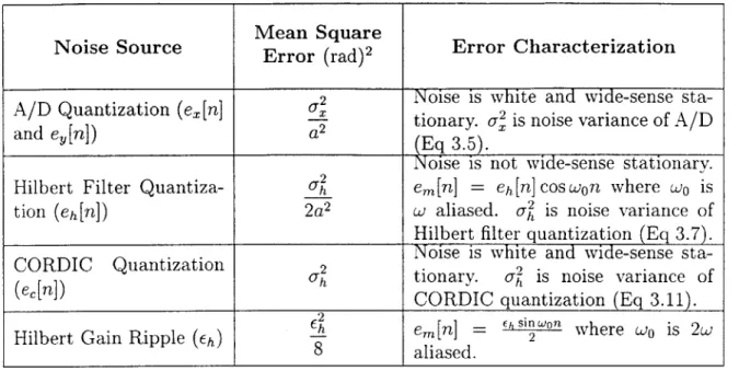
zero-mean, white, and uniformly distributed random process with variance

01 = 2(3.5)X ₁₂

(where B, is the number of fractional bits used to store i[n]). Therefore, the estimate of the position signal, which is labeled i[n] in Figure 3-6, is

1[n] = x[n] + e- [n].

One thing to note is that this noise source looks the same as the White Input Noise case, so their effects will be the same.

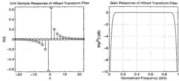
The estimate [], which is the in-phase estimate, is passed through the Hilbert Transform filter to produce the quadrature estimate. If we assume the Hilbert Trans-form filter is an ideal -90' phase shifter, then the true in-phase signal x[n] goes through to produce a perfect quadrature signal y[n] = a[n] sin 0[n]. If the noise e,[n] goes through to produce an output noise ey[n], then the statistics of ey[n] can be ob-tained by considering the characteristics of the Hilbert Transform filter. The Hilbert Transform filter is assumed to be an FIR, anti-symmetric approximation of the ideal Hilbert Transform filtert. As a result, the unit sample response is an odd function, as the example Hilbert Transform filter in Figure 3-7 shows. Because the unit sam-ple response is odd, and because all auto-correlation functions are even, when you convolve them, the sample at time zero will always be zero. Thus, the correlation between e1[n] and ey[n], which is simply

Kexe,[m] = h[m] * Kexej[m], (3.6)

will always be zero for m = 0. This means that samples of the noise in the

in-TFor simplicity the impulse response of the Hilbert Transform filter in this analysis is centered at the origin. In reality it is delayed so that the filter is causal. Since the in-phase signal will be delayed to match the delay of the Hilbert Transform filter, the delay is of no consequence to this analysis. The effects of the delay may be of concern for the specific application, but it does not effect the noise statistics.

Unit Sample Response of Hilbert Transform Filter Gain Response of Hilbert Transform Filter 0.6 0.4 - 2 . . . . .. . . .. . . . . 0.2

00

L...

..

Figure 3-7: Unit Sample and Frequency Response of Hilbert Transform Filter.

phase channel are uncorrelated with their corresponding samples of the noise in the quadrature channel. It does not mean they are completely uncorrelated, but samples at the same time are. This fact will be used later in finding the mean and mean square error of the estimator.

Another property of an FIR Hilbert Transform filter is that it approximates an

all-pass filter. This can be seen in the frequency response of the sample Hilbert

Transform filter shown in Figure 3-7. Because this is the case, the first and second order statistics of ey[n] will approximately match those of e,[n], including the fact

that o ~ o. With ey[n] characterized, we can express the estimate of the quadrature signal as the sum of the true quadrature signal y[n] and the filtered noise e,[n],

Q[n] = y[n] + ey[n],

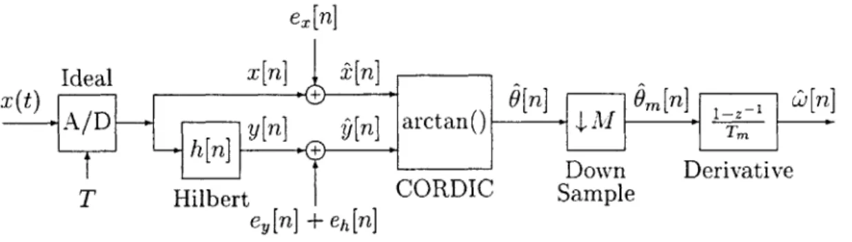
and we can move the noise source ex[n] downstream as shown in Figure 3-8. This, however, is not a complete characterization of y[n] because in reality the Hilbert Transform filter is not ideal and introduces its own quantization noise, and it has gain error.

Hilbert Transformer Quantization Noise

The quantization noise of the Hilbert Transform filter can be isolated to a single place if the filter is implemented in FIR Direct Form (see Reference [7] p.3 6 7). When a filter

is implemented in Direct Form, all the arithmetic can be done without truncating or rounding, and it is only the final output which needs rounded if the word length needs reduced. If the output is rounded to Bh fractional bits, then this quantization can

be represented as an additive noise source which is zero-mean, white, and uniformly distributed with variance

2 -2Bh

0oh = _U- 1 ₁₂ (3.7)

as shown in Figure 3-8. Here eh[n] is the Hilbert Transform filter quantization noise ex[n]

Ideal x[n] [n]

x(t) -[n] Om[n] - w[n]

-n A/ -n 9[n] a arctan( Al M

Down Derivative

T Hilbert CORDIC Sample

ey [n] + eh [n]

Figure 3-8: Vector Readout FM Demodulation with A/D and Hilbert Transformer Quan-tization Noise.

source, and so the quadrature signal estimate becomes

9[n] = y[n] + ey[n] + eh[n].

Note that eh[n] is independent of e,[n] and e[n].

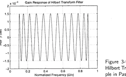
Ripple in the Gain Response of Hilbert Transform Filter

The final effect to consider with the Hilbert Transform filter is that its gain response has ripple on it. This ripple can be made arbitrarily small by increasing the number of taps in the filter, but this adds delay which may be of concern. If the optimum or equiripple FIR filter (see Reference [7] p.486) is used to approximate the ideal Hilbert

Transform filter, then the ripple will be bounded and the gain of the filter over the bandwidth of interest can be expressed as

H(e")l = 1+ Eh

where Ch is the ripple. This ripple is not obvious in Figure 3-7 because it is so small, but in Figure 3-9, the pass band is zoomed to show this ripple. This ripple will have

x 10 - Gain Response of Hilbert Transform Filter

0 0.2 0.4 0.6

Normalized Frequency (Q/t) 0.8

Figure 3-9: Frequency Response of

Hilbert _{Transform Filter Showing}

Rip-ple in Pass Band.

negligible effects on the statistics of ey[n]. However, it will effect y[n], which is the true quadrature signal. The result is that our estimate of the quadrature signal is

Q[n] = (1 + eh)y1[n] + ey[n] + eh[n].

These errors fully represent the intrinsic errors on the quadrature signal estimate.

It was shown in Chapter 2 that the phase response of the Hilbert Transform filter is

exactly -90', so the quadrature estimate will have no phase error on it.

To summarize, we have characterized ,[n] and [n], which are our estimates of the in-phase and quadrature signals. They are

i[n]

S[n]

= a[n]cos 6[n] + e.,[n]

= (1+Eh)a[n]sinO[n] + e,[n] + eh[n].

(3.8) (3.9)

Now we are ready to consider how these noise sources propagate through the CORDIC

2 1.5 0.5 0 -0.5 -1 -1.5 9L -S M ... ... .... .... .... ... .. .... .. .. ... ... . . . . . . . . . . . . . . . . . . . . . .

block and onto the phase estimate.

Quantization Noise of CORDIC

As can be seen from Figure 3-5, the in-phase and quadrature estimates are passed into the CORDIC where it produces an angle estimate. The result is that

O[n] = arctan + n] (3.10)

where ec[n] is the quantization noise of the CORDIC. A rough estimate is that the CORDIC produces about 1 bit of fractional precision for each iteration. Thus, the size of ec[n] _{can be adjusted by changing the number of iterations in the CORDIC,}

but its characteristics change drastically depending on how large ec[n] is compared to the other noise sources on the phase estimate. To see this, consider the case when the noise on the phase measurement is small compared to the quantization noise of the CORDIC. When this is the case, the noise is not well represented as a white random process because it is like sending a saw tooth signal into a A/D converter. However, when the noise on the phase estimate is on the same order or larger than the quantization noise of the CORDIC, it helps to mix things up enough so that the quantization noise looks white. It will generally be desirable that the CORDIC not be the dominant noise source in the system, so for this analysis we assume that ec[n]

is not large compared to the other noise, so it can be represented as a white, zero mean, uniformly distributed random process with variance

2 --2N

-C 12 (3.11)

where N is the number of iterations in the CORDIC algorithm.

Noise Propagated Through the CORDIC

Equation 3.10 shows how the in-phase and quadrature estimates get propagated through the CORDIC. Substituting Equations 3.8 and 3.9 into Equation 3.10 yields

that

(1+Eh) a[n] sin 6[n] + ey[n] + eh[n]

O[n] = arctan ((1±ch) osin] + e,[] + ) + ec[n] (3.12)

a~n cs 6n]+ er[n]

This non-linear relation is not easy to work with, but using a first order Taylor Series expansion of Equation 3.12 to approximate O[n], we obtain

6_{h sin 20[n] ey[n] + eh[n] eEi}

O[n] - 6[n] + + ± an] + cos O[n] - sin O[n] + ec[n]. (3.13)

2 a[n] a[ril

In simulations this approximation has proved to be good (which makes sense because the true in-phase and quadrature signals are the dominant signals), and it is extremely useful because it enables us to treat the CORDIC block as a linear system with respect to the error sources. So we define a new noise source eo[n] which is the sum of all the noise sources in Equation 3.13:

eo[n]-(h sin 20[n]+ e[nj + cos [n] - [n] sin 0[n] + e[c[n] (3.14)

2 a[n] a[n]

This allows us to express the phase estimate as O[n] ~ O[n] + eo[n], and so all the intrinsic noise sources have been moved through the CORDIC as shown in Figure 3-10.

eo [n] - Eh sin 20[n] + (ey nlh [n]) cos 0[n]-e[n] sin O(n] + cn

2 a[n]

Ideal I [n]

x(t) 'O[n] O[n] I- ,,[n]j I__1 [n]

A/D - ~ ]arctan() -o -

-S -h[n] Y - IT

Down Derivative

T Ideal Ideal Sample

Hilbert CORDIC

Figure 3-10: A/D Quantization, Hilbert Gain Error, Hilbert Quantization, and CORDIC