AN ANALYTIC STUDY OF THE BAROCLINIC INSTABILITY PROBLEM ON THE SPHERE
by
YUNG-AN LEE
B.S., Atmospheric Science, National Taiwan University (1979)
SUBMITTED TO THE DEPARTMENT OF
EARTH, ATMOSPHERIC, AND PLANETARY SCIENCES IN PARTIAL FULFILLMENT OF THE
REQUIREMENTS FOR THE DEGREE OF DOCTOR OF PHILOSOPHY
at the
MASSACHUSETTS INSTITUTE OF TECHNOLOGY September, 1987
© Yung-An Lee, 1987
The author hereby grants to M.I.T. permission to reproduce distribute copies of this thesis document in whole or in
and to part
Signature of Author ... ... ... .... ... ...
Department of Ear h, Atmospheric, and Planetary Sciences September, 1987 Certified by... .... . ... ...
Professor Peter H. Stone Thesis Supervisor Accepted by.
irman, Departmental Committee on Gdue Stents Cdairman, Departmental Committele on Graduate Students
by
YUNG-AN LEE
Submitted to the Department of Earth, Atmospheric, and Planetary Sciences on September 4, 1987 in partial fulfillment of the
requirements for the degree of Doctor of Philosophy. ABSTRACT
An analytical study of baroclinic instability on the sphere is presented. We study analogues of both Eady's and Charney's
problems on the sphere. Furthermore, we derive analytic solutions for the problem of a general meridional profile of the basic flow.
The governing equation is the quasigeostrophic potential vorticity equation on the sphere. We adopt a shortwave
approximation and a two-scale assumption to derive the approximate solutions for these problems. These solutions contain a second-order turning point whose location is very important in determining the properties of the unstable waves. This second-order turning point is located at the maximum of the meridional temperature gradient and, because of the variation of the Coriolis parameter, it is always located on the poleward side of the westerly zonal flow maximum.
Furthermore, the analytic solutions indicate a very close relation between baroclinic instability on the sphere and that on a
p3-plane. In fact, if 3-plane is located at the latitude of the turning point, the study of a uniform zonal flow should be able to correctly derive most of the properties of the baroclinic unstable waves on the
sphere. Nonetheless, the spherical geometry and the meridional profile of the basic flow have significant effects on the perturbation's meridional structure and the eddy momentum flux, which can not be correctly predicted by a P-plane study.
Although the analytic solutions have some limitations and are not valid for long waves, they are still able to capture the essential features of baroclinic instability on the sphere. Furthermore, these have implications for parameterizations of the eddy fluxes in climate modeling and allow one to predict the properties of the unstable waves for given meridional profiles of the basic flow, which may be useful for guiding numerical studies.
Thesis Supervisor: Peter H. Stone Title: Professor of Meteorology
To
ACKNOWLEDGEMENTS
I thank my advisor, Professor Peter Stone, for his insights that motivated this thesis. I have benefited greatly from his helpful guidance and suggestions. I also benefited from discussions with Professors Edward Lorenz, Glenn Flierl and Kerry Emanuel. I want to
thank Jane McNabb in Center headquarters and many people in and about Cambridge to whom I am eternally grateful for their advice, support, and friendship during my stay at MIT. As a foreign student, I am grateful for the opportunity to pursue an advanced degree at MIT. During these years, I was supported through National
Page Abstract... ... 2 Dedication...4 Acknowledgements ... ... 5... Table of Contents... ... 6 List of Figures...7 I. Introduction... ... 10
II. The Governing Equation... 21
III. An Analogue of Eady's M odel on the Sphere... 35
IV. An Analogue of Charney's M odel on the Sphere... 50
V. A General Meridional Profile Problem...90
VI. Summary and Conclusion... ... 127
References... ... ... 131
Page Fig. 1.1. The phase speeds(upper) and growth rates(lower) as functions
of the total wavenumber from the exact results(short dashes) of Lindzen and Rosenthal(1981) and the shortwave
approximation(solid), taken from Branscome(1983)...17 Fig. 2.1. The growth rates(a) and phase speeds(b) from Lorenz's
model(solid) and approximated equation(dashes) as function of zonal wavenumber, taken from fig.1 of Hollingsworth, Simmons and Hoskins(1976)... ... ... 27 Fig. 2.2. The perturbation's phases(a) and amplitudes(b) as functions of
latitude from both Lorenz's model(upper) and approximated equation(lower), taken from fig. 2 and fig. 3 of Hollingsworth,
Simmons and Hoskins(1976)...28 Fig. 3.1. The meridional structure of the basic flow as a function of
latitude at z=1... ... ... 45 Fig. 3.2. The growth rate as a function of zonal wave number for each
meridional wave number n, n=1,2,3... ... 48 Fig. 3.3. As in fig. 2.2, except for the steering level...48 Fig. 3.4. The amplitude and phase of the most unstable wave, k=6 and n=1,
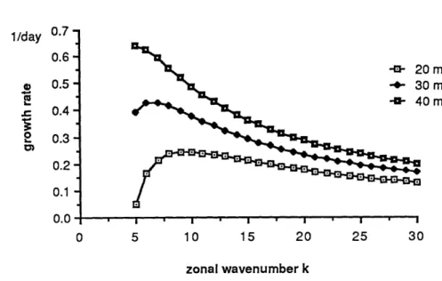
as a function of height...49 Fig. 3.5. The amplitude of the most unstable wave as a function of latitude....49 Fig. 4.1. The perturbation's growth rates for solid body rotation as
functions of the zonal wavenumber k for U0 = 20, 30 and 40 m/sec. NO=- 2x100- -4 sec.-2 and other basic state parameters the same as
chapter iii... ... ... 77 Fig. 4.2. As in Fig. 4.1, except for the phase speeds...77
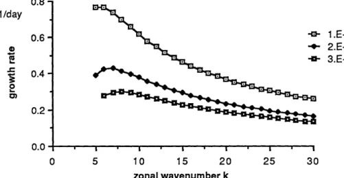
Fig. 4.3. As in Fig. 4.1, except for the cases of N = 1x10 4 , 2x10 4 ,
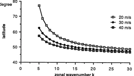
Fig. 4.5. The location of the perturbation's maximum amplitude as a function of the zonal wavenumber k for U0=20, 30 and 40 m/sec.. ... 81
2 -4 -4 -4 -2
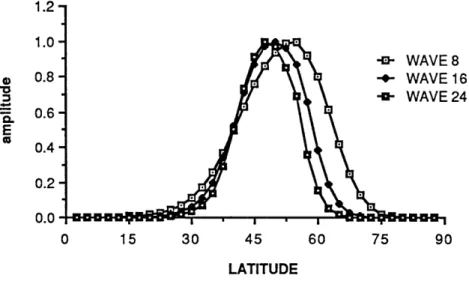
Fig. 4.6. As in Fig. 4.5, except for: NO = 1x10 , 2x10 " , 3x10 sec ... 81 Fig. 4.7. The meridional amplitude functions of k= 8, 16, 24 and n=1
2 -4 2
for U0=30 m/sec. and NO= 2x10⁻⁴ sec. 2 ... ... 82 Fig. 4.8. As in Fig. 4.7, except for the meridional phase variation...82
Fig. 4.9. As in Fig. 4.7, except for the amplitudes as functions of height at the turning point, which is located at 450 latitude...84 Fig. 4.10. As in Fig. 4.7, except for the vertical phase variations... 84 Fig. 4.11. As in Fig. 4.7, except for the eddy momentum fluxes...85 Fig. 4.12. As in Fig. 4.9, except for the eddy heat fluxes at the turning point...85 Fig. 5.1. The meridional cross sections of the basic flows and temperatures for
the 300 jet (a), the 550 jet (b), and for solid body rotation (c), taken from Simmons and Hoskins(1976)... ... 104 Fig. 5.2. The perturbation's growth rates as functions of the zonal
wavenumber for the solid body rotation: the "Short wave" results were calculated from (5.58), the PE and QG results, -taken from Simmons and Hoskins(1976), were calculated from the primitive
equations and the quasigeostrophic equations, respectively... 108 Fig. 5.3. As in fig. 5.2, except for the phase speeds... .... 108 Fig. 5.4. The perturbation's growth rates as functions of the zonal
wavenumber for the 300 jet... 109 Fig. 5.5. As in fig. 5.4, except for the phase speeds... .... 109 Fig. 5.6. The perturbation's growth rates as functions of the zonal
wavenumber for the 550 jet... 110 Fig. 5.7. As in fig. 5.4, except for the phase speeds...110
for the 550 jet. The straight lines are the locations of the turning points for these three profiles... ... 113 Fig. 5.9. The meridional amplitude and phase of the zonal wavenumber 8
as functions of latitude for the solid body rotation...113 Fig. 5.10. As in fig.5.9, except for the 300 jet... 114 Fig. 5.11. As in fig.5.9, except for the 550 jet...114 Fig. 5.12. The perturbation's steering levels at the turning point as functions
of the zonal wavenumber for the solid body rotation, the 300 jet and for the 550 jet...117 Fig. 5.13. The amplitudes of the zonal wavenumber 8 at the turning points
as functions of height for the solid body rotation, the 300 jet and for the 550 jet... 17 Fig 5.14. As in fig. 5.13, except for the leading order phase of the
vertical structure... 118 Fig. 5.15. As in fig. 5.13, except for the eddy heat fluxes... 123 Fig. 5.16. The eddy momentum fluxes of zonal wavenumber 8 as functions of
latitude for the solid body rotation, the 300 jet and for the 550 jet...123 Fig. 5.17. The meridional cross sections of the eddy momentum fluxes at
wavenumber 8 for the 300 jet (a), the 550 jet (b) and for solid body rotation (c), taken from Simmons and Hoskins(1976) ... 124
CHAPTER I
INTRODUCTION
Since the pioneering works of Charney(1947) and Eady(1949), the theoretical study of baroclinic instability has been one of the most important topics in atmospheric dynamics. In the literature, there are two different geometrical assumptions in the studies of baroclinic instability; one is plane geometry and the other is spherical geometry. The difference in geometry has led to somewhat different approaches to studying the problem. Both analytic and numerical analyses have been adopted to investigate the baroclinic instability problem in plane geometry, but only numerical analyses have been used to study this problem on the sphere. Furthermore, although many aspects of baroclinic instability are similar in both geometries, there are some aspects that remain to be understood.
The purposes of this study are: (1). to find an analytic solution for the baroclinic instability problem on the sphere; (2). to learn how the properties of the baroclinic unstable waves on the sphere are determined; (3). to find out the effects of the spherical geometry and the meridional profile of the basic flow on the behavior of these unstable waves.
In the following, we shall discuss the effects of these two geometrical assumptions on the methods applied to study the
(a). the plane geometry
Since the work of Charney(1947), the plane geometry
assumption has been adopted in most of the theoretical studies of baroclinic instability. This assumption neglects the curvature effect
of the earth and the meridional variation of the Coriolis parameter, except that a P-plane is used where the gradient of the Coriolis
parameter is retained. With the quasigeostrophic approximation, the governing equations of the large scale atmospheric motions can be reduced to a single equation, which is the n-plane quasigeostrophic potential vorticity equation. This single governing equation not only simplifies the baroclinic instability problem in plane geometry, but also provides information about the necessary condition for
instability(Charney and Stern, 1962; Pedlosky, 1964a) and bounds on the phase speed and growth rate of the perturbations. Although the plane geometry assumption is unrealistic for the earth's atmosphere, since the baroclinic instability process is mainly a midlatitude
phenomenon, it can still be justified.
For a uniform zonal mean flow, the governing equation of the baroclinic instability problem is a trivial two-dimensional differential equation, which can be easily reduced to an ordinary differential equation for the perturbation's vertical structure. It is easy to solve either analytically or numerically. There are two different models
that were adopted by most of the theoretical studies in plane
geometry; one is Eady's model on a f-plane and the other is Charney's model on a P-plane.
(i). Eady's Model
Eady(1949) introduced the simplest model on a f-plane, where the 1-effect is neglected, that displays the baroclinic instability
process. The basic state of this model has constant density and static stability. The mean flow is a linear function of height without
meridional variation. Since there is no basic state potential vorticity gradient in the governing equation, the necessary condition of
instability can be satisfied if both upper and lower boundaries be horizontal rigid planes. Since the basic state potential vorticity gradient is zero, the equation and the boundary conditions are very simple. Therefore this instability problem can be solved analytically without any difficulty.
The results of this problem show that the instability only occurs at low zonal wavenumbers. Since, as the wave becomes
shorter, the perturbation will be trapped near one of the boundaries, the necessary condition for instability can no longer be satisfied. Therefore, there is a shortwave cutoff for instability. The lowest meridional wavenumber has the largest growth rate. The most unstable wave has a zonal scale similar to the synoptic scale eddies of the atmosphere. The phase speeds are the same for all unstable waves. The unstable waves have the same vertical scale as that of
phase of these unstable waves tilts westward and upward, which is the same condition for the baroclinic conversion of energy from the mean field to the perturbation. Furthermore the eddy heat flux is poleward everywhere. Since the basic flow has no meridional variation, there is no eddy momentum flux in this model.
(ii). Charney's Model
Charney(1947) studied a more realistic model that retains both the f3 term and the vertical variation of the basic state density, which is an exponentially decreasing function of height. The basic state potential vorticity gradient is no longer zero in this model.
Therefore, from the necessary condition for instability, the upper rigid boundary condition can be relaxed and replaced by the radiation condition at infinity.
From the discussion of Held(1978), Branscome(1983) and Pedlosky(1987), the existence of a nonzero basic state potential vorticity gradient has two significant effects on this baroclinic instability problem. One is that there is a singularity in the
governing equation and the other is that there are important changes in the vertical and horizontal scales of the unstable disturbances.
Due to the presence of a singularity in the governing equation, it is more difficult to find an analytic solution for this baroclinic
original work of Charney, they were derived in later studies(Kuo, 1952, 1973; Lindzen and Rosenthal, 1981 and etc.). Nonetheless, these solutions were very complex. It required numerical
calculations to determine the perturbation's growth rate, phase speed and other properties.
Branscome(1983) introduced a shortwave approximation to simplify this baroclinic instability problem. The shortwave
approximation assumes that the perturbation's total wavenumber is larger than other terms in the governing equation. Therefore, after rescaling, the basic state potential vorticity gradient is an order smaller than other terms in the resulting equation. Then he applied
a perturbation method to solve the equation. Since the basic state potential vorticity gradient is not present in the leading order
equation, the perturbation solutions are much easier to find.
Moreover these perturbation solutions are much simpler than the exact solutions. Therefore the properties of the unstable baroclinic waves are more explicit and can be determined without complicated numerical calculations.
Fig. 1.1, taken from Branscome(1983), shows the phase speeds and growth rates as functions of the total wavenumber, which is
scaled by the radius of deformation, from the results of both Lindzen and Rosenthal(1981) and this shortwave approximation. We note that, although these perturbation solutions from the shortwave
Furthermore, we see that only certain neutral points exist in the solutions. There is no shortwave cutoff for instability. This is due to the existence of a nonzero basic state potential vorticity gradient, i.e., as the wave becomes shorter, the vertical scale also shrinks proportionally so that the instability can still occur.
Therefore, in contrast with Eady's model, the presence of the basic state potential vorticity gradient allows the unstable perturbations in Charney's model to select their own vertical scale.
The phase speeds of the unstable waves are near the minimum speed of the basic flow rather than the mean speed as in Eady's
model. The maximum amplitude of the most unstable wave is at the ground. The perturbation's phase variation with height is confined near the surface, so the eddy heat flux is also confined in this region. Since there is no meridional variation in the basic flow, there is no eddy momentum flux.
For a nonuniform zonal flow, the baroclinic instability problem on a plane geometry becomes even more difficult to deal with. Since the basic flow is a function of both vertical and meridional variables, the separation of variables can not be directly applied to the
governing equation. To simplify the problem, a two-scale formalism can be applied to the meridional variable to quasi-separate the equation into a vertical structure equation and a fast variation
meridional equation(Stone, 1969; Gent, 1974; Killworth, 1980; Ioannou and Lindzen, 1986). The perturbation's vertical structure equation is similar to that in the uniform zonal flow problem. The fast variation meridional structure equation is approximated by a WKB equation. Depending on the meridional domain, this equation is
either a simple WKB problem(finite domain) or a two-turning-point problem(infinite domain). Then these two equations can be solved separately to determine the properties of the unstable waves.
The results from these studies showed that, in the presence of horizontal shear in the basic flow, the unstable perturbations would select their own meridional scales. Moreover, there is an eddy momentum flux associated with the unstable baroclinic waves.
Pedlosky(1964b) and Stone(1969) found that this momentum flux is always against the meridional gradient of the basic flow and changes sign at the jet center.
0 1 2 3 K ci O 1 2 3 K/ A I
Fig. 1.1. The phase speeds (upper) and growth rates (lower) as functions of the total wavenumber from the exact results (short dashes) of Lindzen and Rosenthal(1981) and the shortwave approximation (solid), taken from
Branscome(1983). Branscome( 1983).
On the sphere, both the earth's curvature and the full meridional variation of the Coriolis parameter are retained. The
governing equations of the large scale atmospheric motions can not be easily reduced to a single equation. Although Hollingsworth,
Simmons and Hoskins(1976) did introduce a quasigeostrophic potential vorticity equation on the sphere, since its coefficients
depend on both meridional and vertical variables, it is more difficult to solve analytically than that in the plane geometry. Therefore, as yet, there is no analytic study of the baroclinic instability problem on the sphere.
The numerical studies(Hollingsworth, 1975; Moura and Stone, 1976; Simmons and Hoskins, 1976) showed that the eddy momentum flux is an essential feature of baroclinic instability on the sphere.
They found that the stability properties and the structure of the most unstable waves are qualitatively similar to those on a f-plane, but that the spherical geometry has significant effects on the location of the disturbances and on the eddy momentum fluxes, which vary greatly from profile to profile of the basic flow.
Even though the quasigeostrophic approximation formally
breaks down near equator, the quasigeostrophic equations have been used in the numerical studies of baroclinic instability on the sphere. Moura and Stone(1976) found that, since the amplitudes of unstable waves are small near the equator, the unstable solutions of the
Moreover, Simmons and Hoskins(1976) showed that the results from the quasigeostrophic equations are generally similar to those of the primitive equations. Therefore, the quasigeostrophic
approximation does not appear to affect the properties of baroclinic instability on the sphere.
Although a numerical analysis can investigate more realistic atmospheric flows and provide more accurate results for the baroclinic instability problem on the sphere, the determination of cause and effect relationships may be difficult. The existence of the quasigeostrophic potential vorticity equation on the sphere and the introduction of the shortwave approximation by Branscome(1983) gives us an opportunity to analytically study the baroclinic
instability problem on the sphere. With this study we hope to be able to provide a link between the
f3-plane
analytic analyses and the numerical analyses on the sphere. Also, the analytic solutions may be able to provide us information about how the perturbation's growth rate, phase speed, vertical structure, meridional structure, heat and momentum fluxes are determined. These results may be useful in improving parameterizations of the eddy fluxes in climate modeling. Moreover, we may be able to predict the structure of the perturbations for a given meridional profile of the basic flow from these analytic expressions.In chapter ii, we present the derivation of the quasigeostrophic potential vorticity equation on the sphere and discuss the properties
of this equation. In chapter iii, we investigate an analogue of Eady's problem. In chapter iv, we study an analogue of Charney's problem and determine a proper procedure to solve the baroclinic instability problem on the sphere. In chapter v, we study the instability problem for a general meridional profile of the basic flow. In chapter vi, we
THE GOVERNING EQUATION
The governing equation in this study is the quasigeostrophic potential vorticity equation on the sphere, which was introduced by Hollingsworth, Simmons and Hoskins(1976). This equation, except for having coefficients which are explicit functions of latitude, is very
similar to the quasigeostrophic potential vorticity equation on a P-plane. As mentioned in chapter i, the quasigeostrophic
approximation did not have significant effects on the baroclinic instability problem on the sphere, so we adopt this equation as the governing equation in this study. Since there are many analytic studies(Eady, 1949; Kuo, 1952, 1973; Branscome,1983 and etc.) on a P-plane or f-plane, this similarity between the equation on the sphere and that on a P-plane may give us an important clue on how to find an analytical solution on the sphere. In this chapter, we follow the work of Hollingsworth, Simmons and Hoskins(1976) to derive the governing equation and discuss some of its properties.
This governing equation is derived from Lorenz's Model(1960), which conserves the sum of kinetic energy and available potential energy but does not allow the variation of static stability. Since the equations of Lorenz's model are in vector invariant form, they can be presented in spherical coordinates. We introduce 'P as the
streamfunction, X the velocity potential, 0 the geopotential and p the pressure. Then the equations of Lorenz's model can be written as
-- V2T =-J ( ,V2 + f)- V. f VX
at
(2.1) DT -J (P, T)+ o( t( 2.2) V2 - V. f VP (2.3 ) DD RT ap P (2.4) V2X = _ ( 2.5 ) where aT RT S=Y- ( P S) and f = 22g. ap cpHere Ts is the horizontal averaged temperature, t=sin(latitude), R the
gas constant, Cp the specific heat at constant pressure, Q the angular velocity of the sphere and o=dp/dt, the vertical velocity in pressure coordinates. As noted by Hollingsworth et al., this model is
essentially an energetically consistent extension to the sphere of the usual j-plane quasigeostrophic model. On the sphere,
1 aA aB A aB J(A,B)= ( aA B aA B a (2.6) VA
=
A.L (1_2)1/2 ( a ( - 2 )1/2 ak a a3t ( 2.7 )V2A= 1 1 a2A a a A
M2 1 -g2 a2 agL ag
(2.8 )
where a is the radius of the sphere, X the longitude, bold face characters, i and j, the unit vectors in longitudinal and latitudinal directions. By definition, the nondivergent part of wind is a function of the streamfunction; therefore the zonal and meridional parts of it can be written as U -= ( 1 - L2)1 2 DY a ags (2.9 )
a
(1- 2)1( 2.10 )
We linearize the equations by assuming that the
streamfunction and temperature can be separated into -a basic state plus a small perturbation,
(
2.11) T =T (j[, p ) +T'( 2.12 )
From (2.3), (2.4) and (2.9), we can derive the thermal wind relation,
.T fa . au
ag (1-1g2)1/ 2 R
ap
+ ) V2 = = 1 { 2Q - [ u1 ]
at
a(l1- 2)1/ 2 3% a2 ak D2 a + f co - 2 1 - 2 ap a2 ag V2D = V.f V(
2.14
)
( 2.15 )
(2.16
)
(2.17
)
aO RT ap PTo derive a single equation that is analogous to the 3-plane quasigeostrophic potential vorticity equation, two approximations have to be adopted,
( 1 ) neglect 2 1- 2 X in ( 2.14)
2 t
Sa l
(2) replace (2.16) by Q=fY
These approximations were introduced by Dickinson(1968) for the case of vertically propagating planetary waves. As pointed out by
(.+ u )T=- - _au + oco
Hollingsworth et al., the first one implies that the divergent part of the meridional wind is small in comparison with the geostrophic meridional wind, which is consistent with traditional
quasigeostrophic scaling. With regard to the second one, Hollingsworth et al. show that errors introduced by this
approximation are consistent with the usual quasigeostrophic approximation.
From approximation (2) and equation (2.17), we have
T=_ fp-R ap ( 2.18 ) In terms of F, (2.15) yields + u a ) a_.(fp a ) + 1 aT a (fp au ap
a
t
a(1-g 2)1/2 a ap Ro ap a(1-g 2)1/2 , ap Ro ap( 2.19 )
Substituting (2.19) into (2.14) with approximation (1), then we havethe single governing equation on the sphere,
+
,-]
a
)(V2Y +a
fPa__
at
a(1-g 2)1/2 a% apRo ap
+
{ 22
-
[
] -
_1 -(
-
)}
=0
a2 ag2 a (1- 2)1/2 ap
Ro
apTo check if this approximated equation would yield results in good agreement with those of Lorenz's model, Hollingsworth et al. applied both in a two-layer system to study the same baroclinic instability problem. The static stability is taken as a constant. The basic flow is a solid body rotation in the upper layer and a rest state in the lower layer.
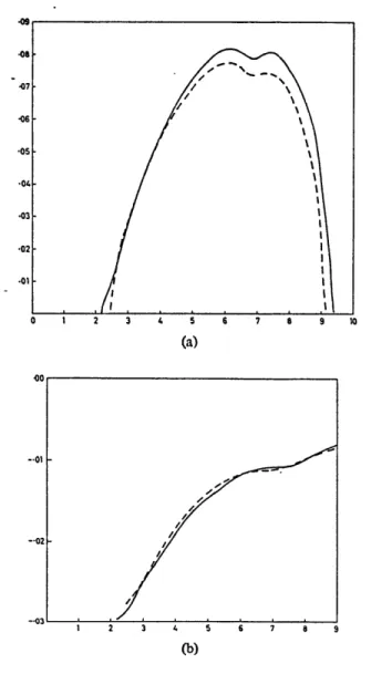
Fig. 2.1, taken from Hollingsworth et al.(1976) fig. 1, shows the growth rates and phase speeds from both models as a function of the perturbation zonal wavenumber. We can see that, in general, the solutions of this approximated equation underestimate the growth rate and overestimate the phase speed. Nonetheless they are in very good agreement even at low wavenumbers where approximation (2) would give a larger error.
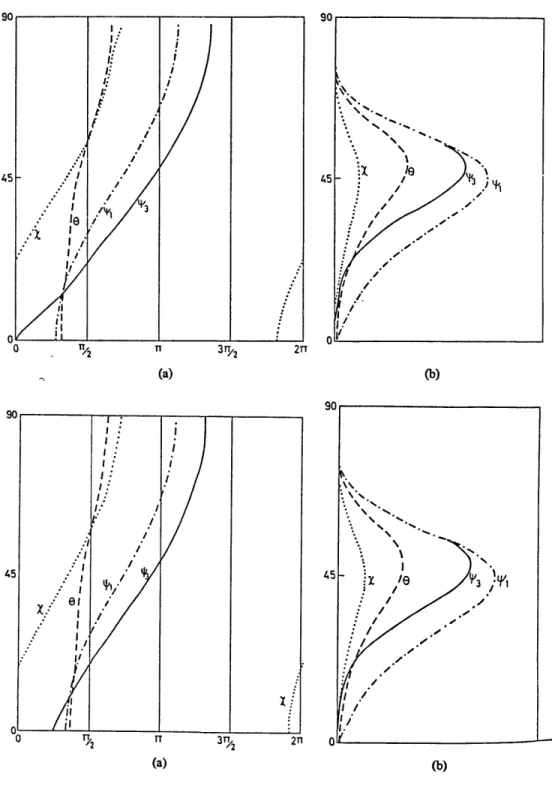
Fig. 2.2, taken from their fig. 2 and fig. 3, show the amplitude and phase of the fastest growing mode as a function of latitude for both models. We note that the amplitudes show little difference between these two models. As for phase, there are some differences near the equator. Since the amplitude is very small near the
equator, these differences are not important.
These results indicate that those approximations that were introduced during the derivation of (2.20) do not have any
Fig. 2.1 The growth rates (a) and phase speeds (b) from Lorenz's model(solid) and approximated equation(dashes) as a function of zonal wavenumber, taken from fig.1 of Hollingsworth, Simmons and Hoskins(1976).
(a) (b)
(a) (b)
Fig. 2.2 The perturbation's phases (a) and amplitudes (b) as a function of latitude from both Lorenz's model(upper) and approximated equation(lower), taken from fig. 2 and fig. 3 of Hollingsworth, Simmons and Hoskins(1976).
To compare with P-plane analyses, we shall change (2.20) from pressure coordinates to height-coordinates and nondimensionalize
the equation. a t=a U 0 u=Ut 0 We introduce z=Hz N2 - L s N2 N2* 0
az
o S V2= 1 V2* 2 awhere ( )* is a nondimensional quantity, H the scale height, Uo the characteristic wind velocity, N2 the Brunt-Vaisala frequency, N
o the
characteristic value of N, g the gravity, and 0s the horizontal
averaged potential temperature. With the aid of the hydrostatic equation, after dropping the stars, the resultant nondimensional equation is ( + U ){ A ( )+ [ t+ - (1-g 2 ) St (1-. 2)1/ 2 a P
az
N2 Z " 2 1-. a2 agag
+ { . _ [(1-g2)1/2 ( -- ) } = 0 ax 9i2 g2 a 2 p(1-g 2)1 / 2 aZ N2 Z ( 2.21 ) The definitions of e and Ps areNH 0 2n a
and
N2H2 s 2QaU 0 ( 2.22 )It is easy to see that e is proportional to the ratio between the radius of deformation and the radius of the sphere, while Ps is analogous to
the P parameter on a P3-plane. For the earth's atmosphere,
2 -2 a- 6400 km, N 2 x 10- 4 sec , 0 H - 8 km, Q= 7.29 x 10- 5 sec 1 U - 30 m sec 0
thus, E=0.1212 and Ps=0.457. We can see that, in general, e is a small quantity and Ps is approximately an order one quantity. If g is
replaced by go, then
a 1 a I 1
ax (1- 2 )112 , ay (1-2)" 1/ 2 g
and we note that the resulting equation is exactly the same as the nondimensional quasigeostrophic potential vorticity equation on a P-plane(from Pedlosky,1987), that is
-+u-
A
){
(Na
2Y )+S2(
+
)}+
{3
2a2u
at
ax
p
az
N
2D
ax
ax ay2 p z2 a zp
az N2
Na ( 2.23 ) where ND S= o0 o IL,,
and
(1-g0)1/2 2D2 o= o g2 29iaU go 0 ( 2.24 )L and D are the perturbation's characteristic horizontal and vertical scales, and go the value of g at 450. Usually both S and
P
are order one quantities for synoptic scale disturbances. Therefore the main difference between these two equations is that the coefficients in (2.21) vary with latitude while those in (2.23) are constants.Since (2.21) is analogous to (2.23), we can apply some results from
f-plane
theory to the sphere. One of them is the necessary condition for instability(Charney and Stern,1962; Pedlosky, 1964a). We assume that the perturbation streamfunction has a normal mode solution,'T
= (g,z) ei(kX - ct)where c is the phase speed and may be complex, and k is the
the equation resulting from (2.21) by pi*, where y* is a complex conjugate of V, and integrate over a meridional cross section. After integration by parts, we have
1 zt 2k2 + 2( -2) } I1 Z a] 00 N2 Z 1- 2
l
1 zt =_JJ
E2 ~ F.2.[(lt2)lu_ -- 2 ( . D U) } )zagl 0 0 - c2 p(s1-2 2)1/ 2 Z N2 Z (1-12)1/2 1 pU2 lwL2 DU z t o N2(1_2)1/2 U -_ Z 0 (1-2)1/2 ( 2.25 )The following boundary conditions have been applied to derive
(2.25), Y = 0 at g=0O, 1 ( 2.26 ) and
a
(1a
aY
1 aY au + U a 0at
(1- 2)1/2 aX aZ (1- t2)1/2 aX aZ at z= 0, z ( 2.27 )If z- oo, the upper boundary condition is taken as Y=0 , then there is no contribution from the integrated term at zt. Since the left hand
be zero. Therefore if there is instability, which means that ci is
positive, then we must require that
1 zt P { - 2 1_
=2)1/2U
( ) } aza f f u a-2 (1-12)1/2p a 2 Z (1-42)1/22
2 + QU au. Z agy =0 o N2( _2)1/2 U 2 Z 0 (1-. 2)1 /2 ( 2.28 )This is the necessary condition for instability on the sphere, which requires that one of the following conditions be met:
(1). the basic state potential vorticity gradient changes sign within the domain;
(2). the basic state potential vorticity gradient term is balanced by the boundary terms at z=0 and z=zt;
(3). the basic state potential vorticity gradient is zero and the boundary terms have opposite signs.
It is easy to see that these conditions are the same as those on a P-plane. We note that baroclinic instability of Charney's and Eady's Models require that either condition (2) or (3) be met. Since the form and properties of (2.21) and (2.23) closely resemble to each other, we can construct spherical models that are analogous to these two. Therefore we may be able to apply some of the methods from
those analytical studies of these two models to solve (2.21) analytically for certain kinds of basic flows. Moreover we can compare them with results from those studies to determine the effect of spherical geometry on baroclinic instability.
CHAPTER III
AN ANALOGUE OF EADY'S MODEL ON THE SPHERE
The simplest model that displays the baroclinic instability process was introduced by Eady(1949). The most significant feature
in Eady's model is that there is no basic state potential vorticity gradient in the governing equation. As noted in the previous
chapter, this feature requires that both upper and lower boundary terms be of opposite sign for instability to occur. Although the absence of the basic state potential vorticity gradient is unrealistic for application to the atmosphere, this model demonstrates the
essential character of baroclinic instability. Therefore, in our analytic study of baroclinic instability on the sphere, we shall begin by
investigating an analogue of the Eady problem.
To derive the analogue of Eady's model on the sphere, we shall assume that Ps is small. Furthermore, p and N2 are taken as
constants. The basic flow has constant vertical shear and has a solid body rotation for the meridional structure, i.e.,
S= ( 1-2)1/2
Z (3.1)
We note that, in (2.21), the important basic flow terms are divided by (1-p2)1/ 2, therefore this flow can be seen as equivalent to
look for the perturbation streamfunction that has a normal mode solution,
' =Re{ e(,z) eik(}-ct)} (1-g2)1/21
(where k=1,2,3,..., is the zonal wavenumb3.2Since the)e is small for
where k=1,2,3,..., is the zonal wavenumber. ' Since e is small for the earth's atmosphere, it can be used as a perturbation parameter. rescale k and ps as
k = e-1 k
-o
and
PS=
S E2 00We
(
3.3
)
where ko and
3
0 are taken as order one quantities. From (2.21), theresulting equation for V is
__
L _
S 0 2_
D2-W 2
"
o+2z)=O
IZ2 i2(1 - 2 ) ta2 ,2 i2 Z-C (3.4)
It is noted that the basic state potential vorticity gradient is O(E2), except near the equator where g approaches zero. Therefore, in general, it is very small in comparison with other terms in (3.4) and will not enter the leading order governing equation. The vertical boundary conditions are
( z-c )-
= 0
These rigid boundaries are required for instability to occur at leading order. For the meridional boundary conditions, we just require that the streamfunction is zero at both the equator and pole,
f= 0 at g= 0, 1 ( 3.6)
We note that if the basic state potential vorticity gradient is neglected, then (3.4) does not contain a term that explicitly depends on both z and [t. If we assume separation of variables, it can be separated into two ordinary differential equations, one for the vertical structure of the perturbation and the other for the
meridional structure. Therefore we assume that y can be separated as
V= O(Z) X(I) 3.7
Substituting (3.7) into (3.4) and neglecting O(e 2) terms, then we have,
- K20 = 0
2 ( 3.8 )
a- -2Q(g)X =
0
(
3.9 )where K2 is a separation function which may depend on g.. The
k2
2 k0 K
Q= { - K2
1-1 2 (32 1 2 ) u
From (3.5) and (3.7), the boundary conditions for 0 are
( 3.10 ) at z = 1 ( 3.11 ) and (1-c) --- = 0 az az at z = 1 ( 3.12 ) As for X, we have at .= 0, 1
( 3.13
)
If K is a constant, then (3.8), (3.11) and (3.12) are all
independent of . and are identical to those of Eady's model. The solution for (3.8) can readily be written as
( = A cosh(Kz) + B sinh(Kz) 3.14
Substituting (3.14) into (3.11) and (3.12), the boundary conditions for ( give
A{(c-1)K sinh K + cosh K} + B{(c-1)K cosh K + sinh K} = 0
( 3.15 )
A + KcB = 0( 3.16 )
For A and B to have nontrivial solutions, we must require that the determinant of the coefficients in (3.15) and (3.16) vanish, which is
2
coth
K 1c -c+ -0
K K2 ( 3.17 )
From (3.17), we can write c as a function of K,
c { ( K - coth K )K tanh K ) 1/2
2 K 2 2 2 2
( 3.18 )
Since c is a constant, K has to be a constant also. We note that if there is instability then c must be complex and the imaginary part of c must be positive. This indicates that the radicand in (3.18) has to
be negative. Since, for all K,
K2 >tanh
-the only possibility for -the radicand being less than zero is that
K < coth K
Therefore, for instability to occur, we must require that
K < K = 2.3994c
( 3.19
)
where Kc is the critical value for instability. We note that, except for K being unknown at this stage, (3.19) is exactly the same condition as that in Eady's problem.
To determine K, we have to find the solution for X. Since e is a small parameter, (3.9) is a standard WKB equation. From (3.10), we note that, if K is less than 2ko then Q is positive everywhere.
Therefore the leading order asymptotic solution for x can readily be written as(Bender and Orszag, 1978),
X D ~x
Q/4exp{
e-fQ1/2 dt}
+ D_ Q1/ 4 expe - 1 Q1/2d( 3.20
)
From (3.13), we know that (3.20) must be zero at both the equator and pole. This requires that both D. and D be zero, therefore there is no nontrivial solution for X. On the other hand, if K > 2ko, then
2 Q= { o0 - K2} = 0, at g= 1 and p=p 2 1-p.2 g2(-. 2) where
( 3.21 )
and k 22-( 1 +4( 0 )2)1/2 2 2 2 K ( 3.22 ) ( 3.23 )
We note that, for this particular basic flow, the squares of , and I 2
are symmetrical about 450 latitude. Since Q=O at these two latitudes, equation (3.9) becomes a standard two-turning-point WKB problem. For g > gl or t < g2, Q is positive, therefore the solution for X is an
exponential function. For g2<p<91, Q is negative, the solution is an
oscillatory function. While near g, or g2, Q is approaching zero, and
the WKB solution does not exist. The solutions in these regions are approximated by Airy functions. To match two one-turning-point solutions in the region g2<1,<g1, a connection condition must be,
satisfied,
(-Q)1/2dg =e(n- 1-)c
2
( 3.24 )
where n= 1, 2, 3,..., is a positive integer. Then the solution for X in each region can be written as
x
-
2 n ( ca 11 )-1/6 A{ e-2/3 a111 (/3-- 1) } for 1- O(e11 2 / 3 ) I5 g 1 + O(E2 / 3 )91
~2(-Q) -1/4 sin( lf (-Q)1/2 dL + 4 ) for g + O(e2 /3) < g < p1 + O(e2/3)
2(-Q)4 2 1 J.L -1/4 1/2 X~ (-1) n+1 Q'2T( exp { e-A1 d}, for)aQ X(-1) n+1 Q 114 f21/2
},
for
g2- O(e2/3) - < [L2t+ O(e2/3) 0 < < L - O(e2/3) ( 3.25 ) where dQ m dLtat
g=g
, m = 1,
2
From (3.24) and (3.25), we can see that n is the meridional wavenumber. For given n and k0o, K is uniquely determined by
(3.24). Therefore, from (3.18), we can determine c. Since K must be less than Kc for instability to occur and must be greater than 2ko for
X to have a nontrivial solution, the unstable range of K is 2ko<K<Kc.
We note that there is a shortwave cutoff for instability as in Eady's model. Moreover as n increases then, from (3.25), K must also increase. Hence for each n there is a different cutoff zonal wavenumber for instability.
From (3.16), we can find B in terms of A, which can not be
determined by linear theory. Therefore, aside from this constant, the vertical structure of the perturbation can be written as
= cosh(Kz) - sinh(Kz)
Kc ( 3.26 )
If the perturbation is unstable, c=cr+c i and ci#0, the amplitude and phase of 0 are c sinh(Kz) 2 c.sinh(Kz)
I1
={
(cosh(Kz)-
r + (i
)2 }1/2Kid
22
Klcl2
KcI
(3.27 )
and = tan -12 c.sinh(Kz) Klc lcosh(Kz) - c sinh(Kz) r ( 3.28 )Since K is a constant, 141 and a are independent of latitude. For given K, 0 is the same as that in Eady's model. The spherical geometry shows no effect on the vertical structure of the perturbation. As for the meridional structure, since Q is real, from (3.25), x is also a real function. There is no meridional variation of phase.
From the solutions of 0 and X, we can write the perturbation
streamfunction as
kcit
1 III e k . ik(k-crt)
= l
_lL
Re{ ee }(1-e2)1/2 ( 3.29 )
Hence the meridional eddy heat flux can be expressed as
2kct
kc.e
=- 1
a
a
, 1x I12(1-g2)1/2 a% Bz 2(1-g 2)3/2c2 (3.30 )
We can see that the heat flux depends on ci. If the wave is neutral,
ci=0, there is no heat flux. If the wave is unstable, then it will
transfer heat poleward. Furthermore this heat flux is independent of height and is proportional to IX12. As for the momentum flux, since the perturbation does not have meridional phase variation, it is identically zero,
uv - -0
a g ( 3.31)
In the following, we shall present some results from above solutions. The basic state parameters, U0, No, 0, a and H, are the
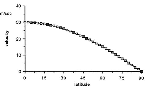
same as in the previous chapter, therefore e=0.1212. Fig. 3.1 shows the meridional structure of the basic flow at upper boundary as a function of latitude. This is a cosine profile with the maximum velocity at the equator and zero at the pole.
40 m/sec 30 o 20 10 0 15 30 45 60 75 90 latitude
Fig. 3.1. The meridional structure of the basic flow as a function of latitude at z=1.
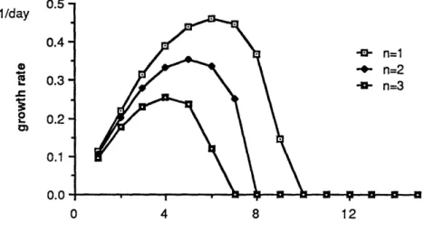
In fig. 3.2, we show the growth rate as a function of zonal wavenumber k for each meridional wavenumber n, n= 1,2,3. It is noted that, for each n, there is a critical zonal wavenumber ke. When
k<kc, the wave is unstable, while for k2kc, there is no instability.
Moreover, as n increases, kc decreases. Comparing the growth rates
for each n, we note that the lowest meridional mode has the largest growth rate. The most unstable wave is k=6, which has a zonal scale about 4500 km. This is very similar to the zonal scale of the most unstable wave in Eady's model. For given n, the scale of the zonal wave that has the maximum growth rate shifts toward longer scales as n increases.
Fig. 3.3 shows the steering level, which is zs=Cr, as a function of k for n=1,2,3. We note that, for unstable waves, the steering levels
are all located at mid level. This also implies that all unstable waves travel at the mean speed of the basic flow, which is exactly the same
as in Eady's model. For neutral waves, depending upon the sign in (3.18), the steering level approaches either the upper or lower boundary as k increases.
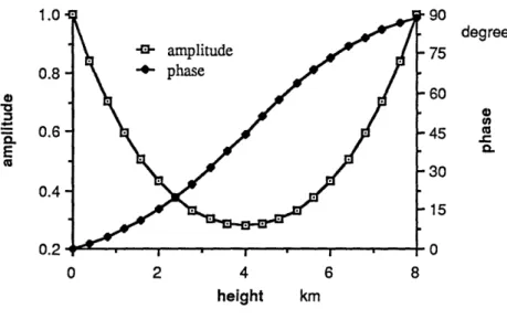
Fig. 3.4 shows the variation of 101 and a with height for the most unstable wave, k=6 and n=l. We can see that
i
is nearly symmetrical about mid level where the minimum amplitude is located. The maxima of141
are located at both upper and lower boundaries. As for a, it is an increasing function of height. This implies that the phase of the wave tilts upward and westward with height, which indicates the conversion of available potential energy of the basic state to the energy of the perturbation. As mentioned in chapter i, for instability to occur, the absence of the basic statepotential vorticity gradient requires that the vertical scale of the unstable wave is the same as the basic flow. Since 0 is independent of i, the vertical structure of the perturbation in any meridional location is the same as that shown in the figure.
In fig. 3.5, we show the amplitude of the most unstable wave as a function of latitude. It is noted that the amplitude peaks near 450 and decays toward both the equator and pole. Since the basic potential vorticity gradient, which will become large near the
as rapidly as it might otherwise. There is no phase variation of the meridional structure.
From the above results we note that this particular case on the sphere is almost identical to Eady's model. The absence of the basic state potential vorticity gradient causes the governing equation to become a separable differential equation. Therefore the spherical geometry only plays the same role as the plane geometry in
determining the meridional structure of the perturbation. It does not have any significant effect on the behavior of the unstable baroclinic wave. Furthermore, since we neglect the basic state potential vorticity gradient in (3.4), the amplitude of the
perturbation in low latitudes may be too large and the eddy
momentum flux does not exist in this case. Therefore, to examine the effect of spherical geometry on baroclinic instability, we should not neglect the basic state potential vorticity gradient, especially the
f
s1/day
o.1
\\ \
0.01 1 1 a IF I
0 4 8 12
zonal wavenumber k
Fig. 3.2. The growth rate as a function of zonal wave number for each meridional wave number n, n=1,2,3.
km M a, C L. a, a,
Fig. 3.3. As in fig. 2.2, except for the steering level.
•
. , I I I I I
0 5 10 15 20 25 30
1.0 0.8 0.6 degree 75 60 45 30 15 0 0 2 4 6 8 height km
Fig. 3.4. The amplitude and phase of the most unstable wave, k=6 and n=l, as a function of height.
0 15 30 45 60 75 90
latitude
Fig. 3.5. The amplitude of the most unstable wave as a function of latitude.
CHAPTER IV
AN ANALOGUE OF CHARNEY'S MODEL ON THE SPHERE
From the previous chapter we note that, without the basic state potential vorticity gradient, there is no significant difference
between the baroclinic instability problem on the sphere and that of Eady's problem. As discussed in chapter i, Charney's model, which includes the P-effect, has been used in many studies to investigate baroclinic instability on a 3-plane. Therefore, to find out the effect of spherical geometry and to develop a proper procedure to solve the baroclinic instability problem on the sphere analytically, we shall study an analogue of Charney's model.
In this chapter, we take Ps as an order one quantity. As in
Charney's model, the static stability, N2, is assumed to be a constant.
The basic state density is an exponentially decreasing function of height,
-z p=e
The basic zonal flow remains the same as that in chapter iii, which is a linear function of height multiplied by a solid body rotation,
U
= (1-g 2)1/2Z (4.1normal mode solution,
S= Re{ y(j,z)ek(-ct)
(1-g12)1/ 2 (4.2)
Substituting (4.2) into (2.21), the resulting governing equation for y is
z2 2 l_ + E 2 + + 1 + } = 0
pZ2
Z 2 2) .2 2 Z-C p2 p2
(4.3 ) Since there is density variation with height, besides the Ps term and
the barotropic term, a baroclinic term which has the value of unity is also present in the basic state potential vorticity gradient. We note that, except for the explicit meridional variations, equation (4.3) is very similar to the governing equation of Charney's problem.
The meridional boundary conditions, which require that the perturbation streamfunction be zero at both the equator and pole, are the same as (3.6),
We assume a horizontal rigid surface at the ground, therefore the lower boundary condition can be written as
c0 + =O
z( 4.5 )
Due to the existence of the basic state potential vorticity gradient, the necessary condition for instability allows us to replace the upper rigid plane with a boundary condition at infinity, which is,
V = 0, as z- oo ( 4.6 )
We note that the vertical boundary conditions, (4.5) and (4.6), do not explicitly depend on g for this particular basic flow and are identical to those of Charney's model.
To examine the effect of spherical geometry on baroclinic instability, we need to be able to determine the properties of the unstable baroclinic waves as explicitly as possible. Although there were many studies of Charney's problem in the past(Charney, 1947; Kuo, 1952, 1973; Lindzen and Rosenthal, 1981; Branscome, 1983, etc.), most of these studies indicated that the analytic solutions of Charney's model are complicated and need a lot of numerical calculations to determine the properties of the unstable baroclinic waves. Furthermore, due to the presence of the basic state potential vorticity gradient, (4.3) depends on both latitude and height and is
more difficult to solve than Charney's problem. Therefore, we have to simplify the problem.
Branscome(1983) introduced a shortwave approximation to study Charney's problem. As discussed in chapter i, by using this shortwave approximation, the basic state potential vorticity gradient did not enter the leading order equation. Therefore, the solutions were easier to find and simpler. Moreover, the properties of the unstable baroclinic waves could be determined without any
complicated calculations. Though these perturbation solutions are not valid for the whole zonal wave spectrum, in comparison with the exact solution, they do give reasonable results even at synoptic scale wavenumbers.
We shall apply this approximation to simplify the problem by assuming that the perturbation's zonal wavenumber is O(e-2). Since the short waves are shallow, we rescale k, z and c as
k= e-2k , z =
e1 and c= e c'
where k0, C and c' are taken as order one quantities. In terms of 5,
after dropping the prime of c', (4.3) and (4.5) become,
k..4 4l+ +1+ }=0
DC2 - 2(1-_g2) E12 9 2 -C 12 412
c ++
=0
(4.9)
We note that the basic state potential vorticity gradient is O(e)
smaller than other terms in (4.8), therefore it does not appear in the
leading order perturbation equation.
Because of the existence of the
Ps term, which depends on both p. and
,
we can not directly apply
separation of variables to (4.8) as in chapter iii.
Instead, we shall
apply a two-scale formalism to the meridional variable to separate
the perturbation's fast variation meridional structure from the
vertical structure.
We assume that N has two different meridional
scales and can be written as
V = (,L,4) x() ( 4.10 )
where rl is the fast variation meridional scale. In order to retain the
g. variations to lowest order so that the boundary conditions in . can
be satisfied, the meridional variations must be even more rapid than in the Eady problem, and we must define
l = -21 ( 4.11
)
x is the principle meridional structure of the perturbation and 0 is the vertical structure with slow meridional variation. Furthermore, we assume that the governing equation for X is
-%n
2
Dg
2
a42-27
Ea 2 -QZ=0( 4.12
)
where
Q
is an unknown function of p. and will be determined by
solving the vertical structure equation.
From (4.10) and (4.12), the g
derivative term in (4.8) becomes
2 l 2
X
all a~ aSubstituting (4.10) and (4.13) into (4.8), we have the governing equation for , which is
12
-2- 3 D -K20++C +a) L2(1-12) pL2 {X 2F a a +1-I. a+}2
+ F6 (b+ -L- )=0
-c 2 ( 4.14 )
where we define that,
( 4.13 ) k" K2 = 0 _ Q2 9.2(1- 2) g 2 b= +1 2
Since
Q
is unknown, K is also an unknown function of g. b is the
leading order basic state potential vorticity gradient.and
( 4.15 )
( 4.16 )
(4.12) is a standard WKB equation and its asymptotic solution can be written as X'~ exp{ E -2 e2nqn d } n=O ( 4.17 ) where 2 2 dq q =Q, 2q0ql+ - =0, d( 4.18 ) and 2q q + dq-q + n2 2. d t •- in-i - ( 4.19 )
With (4.17), the rl derivative term in (4.14) can be calculated as
1 . =Z 2n
qn
X n= n (4.20 )
Therefore 0 does not really depend on x or rl. If Q is not an order one quantity somewhere in the meridional domain, then this two-scale expansion will not be valid near that location. We need to apply a local expansion to solve (4.8) in that region.
From (4.6), (4.9) and (4.10), the boundary conditions for 0 are,
c -+0=0, at C=0
¢=
0as
-) oo
( 4.22 )For X, the boundary conditions are
X=0, at V=O0,1
( 4.23
)
We note that there are two unknowns, K and c, in these equations. By requiring that (4.21) and (4.22) be satisfied by the solution of (4.14), we can find K as a function of c. Once K is known, from (4.15), we can determine Q. Since K is a function of c, Q will also depend on c. Then c is determined by requiring that X meet the boundary condition (4.23).
In the following, we shall apply a perturbation method to solve (4.14). We assume that 00oo n=O n=o C = en n and n=O ( 4.24 ) Since, if co is real there is a singularity at C=co, we need an inner
equation to properly describe the behavior of 0 near this layer. We introduce an inner variable,
=EI(-C0) (4.25 )
00
K= I nK
In terms of , (4.14) becomes
-& - -_ 2K2 + 4i 2b { 1+ ec } + O(e4 ) = 0
2 D4 4_C 4-C
( 4.26 )
where i is the inner solution for the vertical structure and can be expressed in the same form as 0 in (4.24).
The leading order perturbation equations and boundary conditions are, 0-K20 =L 0 0 ( 4.27 )
c
-
+
0=0,
at C=O
S0=1= 2= ... =0,as
-- oo ( 4.28 ) ( 4.29 ) and - L0i
=0 2 00 ( 4.30 )We note that these equations do not explicitly depend on pL. After satisfying the upper boundary condition, the solution of (4.27) can be written as
-Ko ( -c)
where Ao is a constant. We lose no generality by taking Ao to be
independent of p., because any such dependence can be absorbed in X. The lower boundary condition (4.28) requires that
1 K =1
OC
( 4.32 )
Since co is a constant, Ko has to be a constant also. This implies that
%
is just a simple exponentially decreasing function of height and does not vary with latitude. Furthermore, since Ko is a constant, the leading order vertical scale does not vary with latitude. The solution of (4.30) is A +B. Since, in terms of , the leading order of (4.31) is just A0, therefore A=0 and B=Ao, and the leading order inner solutionis
i =A
o o0
( 4.33
)
Except for the fact that Ko is unknown at this stage, these leading
order solutions are the same as those of Branscome(1983).
The first order equations for O and
4O
can be written as0o bo L-
o0
=-+2KK a1 0 ---- -C = L1 000 0 and 0 1 ( 4.34 )( 4.35
)
The lower boundary condition for ,1 is
-1 = -To0
0 - 1 - 1
(
4.36 )
The only difference between these equations and those of
Branscome(1983) is the existence of the 2KoK 1 term in (4.34). From
Hildebrand(1976), the particular solution of ,1 can be found as
e-K
0(
- co) 2K-c -K(x-c= ee L1 od x } d4
r S ( 4.37 )
After integration, the solution for 1 is
-Ko ( -co) 1 = Aoe {(- K1) 2 1
b
2Ko(;-c) + - [e E ( 2Ko( -c) ) + In K o(-c ) ] } 2K 1 0 ( 4.38 )where the definition of El(x) is(Abramowitz and Stegun, 1964)
E (x) = e dt, x 0 x t
x (4.39 )
and
E.(x)
= e dt, t -X x>0 ( 4.41 )Therefore, if C < co, 01 will be complex. This feature is due to the existence of the basic state potential vorticity gradient. Since we look for instability, we shall only choose the positive sign in (4.40). The lower boundary condition yields
K + be 2E (-2) - K2c - K2c - be 2( E(2)- i)
1 2 1 o 1 2 o 1
E(2)
( 4.42 )
K, is a complex function. Since b varies with 1/g2, K1 also varies with 1/g2. In terms of , the first two orders of
p
can be approximated as11 b + = A 1 + e{ -K
+
-(--K)-- (E +In 2) o 10K 2 2K 0 0 0 K2 .2 E + In 2 -1 + 82 o _ eb (IneK + 0 2 0 2 (4.43 )where Eo = 0.5772..., is Euler's constant. It is noted that if < 0, then
( 4.44 ) In = In (-4) - in
The general solution of (4.35) is also A +B. After matching with (4.43), we can determine A and B. Therefore the first order inner solution is
= A {-K + (K2C - be-2 E (-2) b (E + In 2))}
1 o K 0 o 1 2 o
( 4.45 )
Since (4.38) and (4.45) depend on b, they will vary with latitude. Except for b being a function of g, these solutions are virtually identical to those of Branscome(1983).
The second order perturbation equations for
4
and gi are02 1 0 2 1 0g 2
X T
a" (b-Co)2 = L 1+ L ( 4.46 ) andL
1 =. + K20i 0 0 2 0 0 -C1The lower boundary condition for 0 is
Do
o ao
c + =-c - c 0
0 D 2 1 D 2 DC
( 4.47 )