Analytical and Simulation Models for Flexible,
Robotic Automotive Assembly Lines
by
Yi-Shiuan Tung
Submitted to the
Department of Electrical Engineering and Computer Science
in partial fulfillment of the requirements for the degree of
Master of Engineering in Electrical Engineering and Computer Science
at the
Massachusetts Institute of Technology
June 2018
c
○ Massachusetts Institute of Technology 2018. All rights reserved.
Author . . . .
Department of Electrical Engineering and Computer Science
May 12, 2018
Certified by . . . .
Julie A. Shah
Associate Professor
Thesis Supervisor
Accepted by . . . .
Katrina LaCurts
Chair, Master of Engineering Thesis Committee
Analytical and Simulation Models for Flexible, Robotic
Automotive Assembly Lines
by
Yi-Shiuan Tung
Submitted to the Department of Electrical Engineering and Computer Science on May 12, 2018, in partial fulfillment of the
requirements for the degree of
Master of Engineering in Electrical Engineering and Computer Science
Abstract
To adapt to the rapidly changing market, the automotive industry is interested in flexible assembly lines that can handle disruptions due to machine failures or schedule changes. In this thesis, we propose a new assembly line layout (flexible layout) that uses mobile, robotic platforms to transport cars, which can move out of the line when disruptions occur to prevent blocking other cars on the line. We use discrete event simulation and analytical models to analyze the throughput of the new layout in a single band and two bands with a finite buffer. The simulation results show that the new layout achieves an average of 25.6% and 35.9% speed up over the conventional layout for the single band and two bands cases respectively. We improve previous two-machine line analytical models by augmenting the state of the Markov chain to model every machine in a band. We show that the augmented discrete Markov chain model predicts the throughput within 13% and 18% of the simulation throughput for the conventional and flexible layouts respectively. We further evaluate whether the flexible layout can improve its throughput by learning a policy for parking the platforms. By modeling the agents as independent learners, we apply single-agent reinforcement learning algorithms and show that the policy learned works well but suffers from lack of coordination.
Thesis Supervisor: Julie A. Shah Title: Associate Professor
Acknowledgments
I’d like to thank my parents for their continued support in my studies and career. I worked as a software engineer at a start up before returning to finish my masters degree, and through this process, my family has been supportive of my decisions and continues to encourage me to pursue my interests.
I’d also like to thank my advisor, Prof. Julie Shah, for her guidance and support. Even with her busy schedule, she found time to discuss my progress and provide feedback on a regular basis. She was passionate and excited about the work and was always encouraging especially when progress has stalled. She has taught me to be an independent thinker and given me opportunities to challenge myself. Besides advising my work, she has gone above and beyond to provide help on my resume and job search as well as discuss career opportunities. I am deeply grateful for her commitment to her students.
Last but not least, I’d like to thank the members of IRG for providing a fun and welcoming environment. I enjoyed the lunch discussions, coffee runs, sports activities, and other social events we had. I also thank IRG for the insightful discussions and suggestions for this project.
Contents
1 Introduction 9
2 Simulation of Automotive Assembly Line 15
2.1 Conventional Automotive Assembly Line . . . 16
2.1.1 Definitions . . . 17
2.1.2 Algorithm . . . 19
2.2 Flexible Automotive Assembly Line . . . 21
2.2.1 Definitions . . . 24
2.2.2 Algorithm . . . 27
2.2.3 Scheduling and Rescheduling . . . 29
2.3 Multi-Band Simulation . . . 32 2.3.1 Definitions . . . 32 2.3.2 Algorithm . . . 33 2.4 Experiments . . . 34 2.4.1 Dataset . . . 35 2.4.2 Comparison Design . . . 36
2.5 Results & Discussion . . . 36
2.5.1 Single Band . . . 37
2.5.2 Two-Band . . . 38
2.5.3 Limitations . . . 44
3 Analytical Models of Automotive Assembly Line 45 3.1 Definitions . . . 46
3.2 Overview . . . 49
3.3 Single Band Analytical Models . . . 52
3.3.1 Conventional Layout . . . 53
3.3.2 Flexible Layout . . . 60
3.4 Two-Band Analytical Models . . . 63
3.4.1 Conventional Layout . . . 64 3.4.2 Flexible Layout . . . 75 3.5 Parameter Estimation . . . 78 3.5.1 Service . . . 78 3.5.2 Failure . . . 79 3.5.3 Repair . . . 80
3.6 Results & Discussion . . . 82
3.6.1 Single Band . . . 83
3.6.2 Two-Band . . . 86
4 Policy Learning for Parking of Mobile Platforms 91 4.1 Background . . . 92
4.2 Preliminaries . . . 94
4.3 Problem Formulation . . . 97
4.4 Policy Iteration . . . 98
4.4.1 State Representation and Reward Function . . . 99
4.5 Q-Learning . . . 100
4.5.1 State Representation and Reward Function . . . 102
4.6 Results & Discussion . . . 102
5 Conclusion 107
Chapter 1
Introduction
Recent challenges in the automotive industry are the frequent change in customer demands, assembly technologies, and introduction of new models and materials. In order to stay competitive in a global market, the manufacturing process is transition-ing from mass production to mass customization. One of the main challenges is the need for faster ramp-up processes to adapt to the changing market [38], which can be achieved by establishing a flexible production system [16]. Previous work identified four areas of manufacturing flexibility: volume flexibility, variety flexibility, process flexibility, and material handling flexibility [13]. In this work, we present a new as-sembly line layout that addresses process flexibility which is the ability of the system to handle changes and disruptions in the manufacturing process, such as machine failures or scheduling changes.
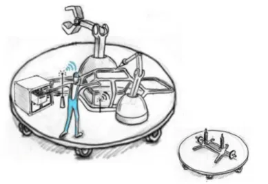
The proposed layout uses mobile platforms to transport cars in a band. Figure 1-1 shows a sketch of a mobile platform. In the current layout, the cars are transported on a line similar to a conveyor belt. The band is divided into work stations where specific tasks are performed. When a car requires more time at a particular station due to disruptions, the entire band pauses until issues are resolved. The proposed layout, which we refer to as the flexible layout, gives a car the flexibility to move to different tracks or move out of the line when disruptions occur. The flexible layout requires the following major changes: 1. equipment are placed on the platforms, 2. logistics are either placed on the platforms or moved along the platforms by
Figure 1-1: Mobile platform that carries cars through a band. Agents perform tasks with equipment on the platform. Supplies may be carried by an autonomous guided vehicle (AGV). Courtesy of BMW.
autonomous systems such as automatic guided vehicles (AGVs) [38] and 3. workers are required to perform multiple different assembly tasks. While further study is required to determine which sections of the assembly line is able to accommodate the above changes, we study how such a layout is able to mitigate the disruptions on the line. The rest of the thesis is structured as follows: Chapter 2 uses discrete event simulation to compare the performance of the conventional and flexible layouts, Chapter 3 presents analytical models for throughput prediction, Chapter 4 evaluates whether a policy can be learned to optimize the movement of mobile platforms, and Chapter 5 presents the conclusions and suggestions for future work.
In Chapter 2, we use discrete event simulation (DES) to compare the throughput performance of the layouts. Simulation has been used widely for assembly system design and performance analysis, and DES is a popular technique because of the discrete nature of assembly lines [43]. DES has been reported to be used in over 40% of papers in manufacturing and business and is appropriate for process analysis, resource utilization, queuing, and more short term analyses [26]. We built off of previously developed DES of the conventional and flexible layouts which uses the Java programming language [28]. The simulation has three components: pre-processor, scheduler, and simulator. First, the pre-processor merges simultaneous and immediate
temporal constraints to simplify scheduling. Then in each cycle of the manufacturing process, the scheduler greedily assigns tasks to stations and agents, and the simulator keeps track of the overall state of the band. Because the optimal schedule is NP-complete [28], the scheduler uses a greedy algorithm to speed up the simulation. We use collected data from a BMW plant to simulate the disruptions. In the conventional layout, the line stops if a station experiences an error; otherwise, the car won’t be able to finish assigned tasks at its current station. In the flexible layout, the mobile platform can move to a parking station, but if accessible parking stations are full, the line stops for a whole cycle. We evaluate the two layouts by the throughput, or units produced per hour, for the single band case and the two-band with one buffer case. We show that the flexible layout achieves an average of 25.6% speed up over the conventional layout for the single band case and an average of 35.9% speed up for the two-band case with a buffer size of 10.
In Chapter 3, we present analytical models for the throughput analyses of con-ventional and flexible layouts. Because simulation has relatively long implementation time and large computational costs, analytical models are sometimes preferred as an initial evaluation of an assembly line design. Previous work has demonstrated the importance of analytical models in throughput analysis [31]. However, due to the large state space of assembly line systems, exact models only exist for two-machine lines [30]. The performance of longer lines are approximated by using two-machine lines as building blocks such as aggregation methods [33] and decomposition methods [19]. We limit our study to single and two-machine lines. Li et al. reviewed liter-ature on throughput analysis of large volume production systems with serial lines, assembly/disassembly systems, parallel lines, among many others [31]. For serial two-machine lines [30], analytical models are classified into synchronized with time-dependent failure mode [25, 7, 32], synchronized with operation-time-dependent failure mode [7, 18], asynchronized with time-dependent failure mode [25], and asynchro-nized with operation-dependent failure mode [18, 1]. The uptimes and downtimes of machines are geometrically distributed in synchronized models and exponentially distributed in asynchronized models. Other types of distributions such as Erlang
and phase-type are analyzed in [23, 2]. We only consider geometric and exponential uptimes and downtimes and estimate the parameters using the maximum likelihood estimator.
Based on data collected, the conventional layout is modeled with operation-dep-endent failures, and the flexible layout is modeled with time-depoperation-dep-endent failures. Sim-ilar to existing methods, we use Markov chain to represent the state of the line and solve for the steady state vector to calculate throughput. However, instead of only modeling the state of a single machine, we model the states of every machine in the band. For the single band case, the state of the line is represented by the number of machines in error. For the two-band case, the state of the line is represented by the tuple (𝑆𝑢, 𝑆𝑑, 𝑖) where 𝑆𝑢 and 𝑆𝑑 are the number of machines in error in the
up-stream and downup-stream bands respectively, and 𝑖 is the number of cars in the buffer. We evaluate discrete models with geometric uptimes and downtimes and continuous models with exponential/gamma uptimes and downtimes. Our results show that the discrete Markov chain model has the best throughput prediction for the single band conventional layout with less than 8% error, and Buzacott’s analysis [4] has the best throughput prediction for the single band flexible layout with less than 13% error. For the two band case, the discrete Markov chain model has best predictions in most cases, with less than 11% and 18% error for the conventional and flexible layouts respectively.
In Chapter 4, we evaluate whether single-agent reinforcement learning (RL) al-gorithms can be used to learn a policy for moving mobile platforms (MPs) that are in error. In DES, we used a greedy algorithm which moves MPs that are in error to adjacent parking stations. If adjacent parking stations are occupied, the algorithms checks whether the currently parked MPs can move. While this algorithm is simple and works well most of the time, it is not optimal. First, it doesn’t consider the number of cycles left and whether moving the MP to a parking station is necessary. Second, it does not prioritize MPs. Besides trying to improve the greedy algorithm, we’re also interested in investigating applying RL algorithms to a stochastic multi-agent system with tightly coupled multi-agents. We formulate the MPs (multi-agents) as
inde-pendent learners where each agent considers other agents as part of the environment. To achieve this, the agents take actions in a predetermined order to avoid collisions due to miscoordination. We evaluate a planning algorithm, policy iteration, and a learning algorithm, Q-learning with function approximation [17]. In policy iteration, the system is modeled as a factored decentralized Markov decision process to reduce the state and action space. Each agent only observes its own state and the states of the adjacent stations. In Q-learning, the system is modeled as a multiagent Markov decision process where agents can observe the full state of the band and take actions individually. We use function approximation to avoid the high memory consumption of storing state, action values in a table. We show that the policies learned by policy iteration and Q-learning perform similarly to the greedy algorithm, but the greedy algorithm performs better in some cases where coordination is required.
Single agent RL algorithms have achieved wide success in problems ranging from game playing [42] to robotics [20]. However, for multiagent systems, RL algorithms suffer from miscoordination, non-stationarity, and high variance in observed rewards. For fully cooperative systems, Team Q-learning augments the Q-value with joint ac-tion and makes updates with joint rewards [35]. Team Q-learning is infeasible for large number of agents because the action space is exponential in the number of agents. Distributed Q-learning makes the optimistic assumption and only updates a state, action value if the observed reward plus the discounted next state’s value is greater than the current value estimation [29]. However, the optimistic assump-tion only works for deterministic environments. Previous work in multiagent coor-dination includes distributed constraint optimization [14], approximate joint action values [22, 21], heuristics in exploration strategies [9, 8, 27], and attempts to reduce coordination set [46, 11]. Some recent work are in the deep learning domain. An actor-critic algorithm augments the state space such that the policies of the other agents are considered [36]. This approach aims to solve the non-stationarity problem by explicitly modeling the policies of other agents. Another work attempts to solve the non-stationarity and high variance problems by using importance sampling and adding iteration number on training data to stabilize experience replay. Because of
the tightly coupled agents in our environment, we avoid coordination and formulate the agents as independent learners so that single agent RL algorithms can be applied. In Chapter 5, we summarize the main contributions in this thesis. We discuss the benefits of the flexible layout as well as identify the limitations of our analyses. We also provide suggestions for future work.
Chapter 2
Simulation of Automotive Assembly
Line
We use discrete event simulation (DES) to analyze the throughput of the conven-tional and flexible automotive assembly lines. DES models a system as a state ma-chine where the state can change instantaneously at discrete time intervals [44]. In contrast, continuous simulation models a dynamic system where the state changes continuously with time, and the behavior can often be represented by differential equations. Because of the discrete nature of events in assembly lines, such as com-pletion or assignment of tasks, DES is more appropriate for modeling assembly lines and other material flow systems for throughput analyses.
The automotive assembly line process typically involves four stages: stamping, body shop, paint and final assembly [38]. We model a single band in the final assembly stage with real data collected from a BMW plant. The single band models are built off of previous work from [28] with some differences in assumptions. Sections 2.1 and 2.2 describe the conventional and flexible layouts respectively. Our main contribution is discussed in Section 2.3, where we extend the single band models to two bands with a single buffer. We report the throughput comparison of the two layouts in Section 2.5. Our simulation shows that the single band line with flexible layout achieves a 25.6% increase in throughput over the conventional layout, and the two-band line with a buffer capacity of ten with flexible layout achieves a 35.9% increase in throughput
over the conventional layout.
2.1
Conventional Automotive Assembly Line
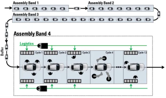
The conventional layout was first introduced by Henry Ford for the mass production of the Model T and has since been adopted by many industries. For the automotive assembly line, the layout consists of a single or multiple linear lines of stations. Each station has one or more agents who perform a set of tasks. The line is divided into sections called bands, which are connected to each other by buffer zones. Generally, no tasks are performed in the buffer zones, and they are used to decouple bands such that a slow down in one does not immediately propagate to another. More details about the buffer are discussed in Section 2.3.
Each band can be viewed as an individual conveyor belt that moves at a constant speed, so agents have a fixed amount of time, known as the cycle time, to complete their tasks at a given station. If an agent needs more time, the entire band stops until the task is completed. Figure 2-1 shows an illustration of the conventional layout.
Figure 2-1: In the conventional layout, the cars move on the assembly line, which is separated into bands. The buffers connect the bands and serve to decouple bands from each other. Courtesy of BMW.
We make the following assumptions in our model:
∙ The band stops when an error occurs at one of the stations in the band and only moves again once the error is resolved. The stations may continue to work on tasks when the band stops but become idle if the task is completed before the error is resolved.
∙ Errors are operation-dependent, meaning that errors can only occur when a task is being executed. [6] reported that operation dependent, single station failures are the most frequently observed types of errors.
∙ Each station has a probability 𝑝 of experiencing an error per cycle. 𝑝 is chosen from observed data and is the average number of errors in a station per working cycle. We assume at most one error can occur in a cycle.
∙ Agents are assigned to a single station for the entirety of the production process. We assume that all agents are able to execute the tasks at the station as well as resolve all errors. We consider anonymous agents and do not take into account their skill set or expertise for the assignment of tasks.
First, we provide definitions for the components of our model in Section 2.1.1. In Section 2.1.2, we provide an overview of the algorithm.
2.1.1
Definitions
Band 𝑏 < 𝑆𝑏, 𝑣𝑏 >
A band 𝑏 is a section of the assembly line that consists of 𝑛 stations 𝑆𝑏 = {𝑠1...𝑠𝑛} of
equal length 𝑙. The band moves cars at a constant speed 𝑣𝑏 but can be stopped by
an agent if necessary. Cars enter the band at station 𝑠1 and exit at station 𝑠𝑛. The
cycle time 𝑡𝑐 is the time it takes for a car to traverse a single station of the band if
the band is not stopped, 𝑡𝑐= 𝑛×𝑙𝑣
Station 𝑠 < 𝑊𝑠, 𝐴𝑠 >
A station consists of a set of agents 𝐴𝑠 and a set of tasks 𝑊𝑠 that it can handle.
At most one car can occupy a given station at any point in time, and one or two agents can be assigned to a given station. In our model, agents are assigned to a single station and do not move to other stations during production. A car only visits a station once, therefore all tasks 𝑊𝑐 for car 𝑐 that is in 𝑊𝑠 are performed in a single
cycle.
Task 𝑤 < 𝑑𝑤, 𝑠𝑤, 𝑛𝑤, 𝑠𝑡𝑤, 𝑒𝑡𝑤 >
The assembly process for a car 𝑐 is divided into tasks 𝑊𝑐where each 𝑤 ∈ 𝑊𝑐has a fixed
duration 𝑑𝑤(time to complete the task), a station 𝑠𝑤 where the task is performed, and
the number of agents 𝑛𝑤required to perform the task. In our model, the task duration
is deterministic. When a task is scheduled, the time the task begins execution 𝑠𝑡𝑤
and the time the task is completed 𝑒𝑡𝑤 are determined.
Agent 𝑎 < 𝑠𝑎>
An agent is assigned to a specific station 𝑠 and stays at that station for the entirety of the production process. We assume all agents assigned to station 𝑠 can perform the set of tasks 𝑊𝑠 at 𝑠 and can resolve all errors.
Car 𝑐 < 𝑊𝑐, 𝑚𝑠𝑐>
A car 𝑐 consists of a set of tasks 𝑊𝑐 that has to be completed in the band. The sum
of task duration is the makespan 𝑚𝑠𝑐, 𝑚𝑠𝑐 =
∑︀
𝑤∈𝑊𝑐𝑑𝑢𝑟𝑎𝑡𝑖𝑜𝑛(𝑤). We consider the
production of cars with variety and customization, so 𝑊𝑐 may be different for each
car 𝑐.
Temporal Constraints 𝛼𝑖𝑗 ≤ 𝑡𝑗 − 𝑡𝑖 ≤ 𝛽𝑖𝑗
Temporal constraints or precedence constraints encode the order that tasks have to be executed. We represent the constraints as simple temporal constraints (STC),
which have the form 𝛼𝑖𝑗 ≤ 𝑡𝑗− 𝑡𝑖 ≤ 𝛽𝑖𝑗 for two time points 𝑡𝑗 and 𝑡𝑖 and a lower and
upper bound [𝛼𝑖𝑗, 𝛽𝑖𝑗]. Let 𝐴 and 𝐵 be any two tasks with start times 𝑠𝑡𝐴 and 𝑠𝑡𝐵
and end times 𝑒𝑡𝐴 and 𝑒𝑡𝐵 respectively. In our model, there are three ways that 𝐵
can be constrained by 𝐴:
Delay Constraint: 𝐵 can only begin execution after 𝐴 has been completed for at least some time 𝛼𝐵𝐴. The execution of 𝐵 is delayed by 𝛼𝐵𝐴 after A is completed. In
STC, these constraints have the form 𝛼𝐵𝐴 ≤ 𝑠𝑡𝐵− 𝑒𝑡𝐴 ≤ ∞. Note that there is no
upper bound in delay constraints.
Immediate Constraint: 𝐵 has to be executed immediately after 𝐴 is completed. In STC, these constraints have the form 0 ≤ 𝑠𝑡𝐵− 𝑒𝑡𝐴≤ 0.
Simultaneous Constraint: 𝐵 starts execution at the same time as 𝐴. The two tasks have to start simultaneously. In STC, these constraints have the form 0 ≤ 𝑠𝑡𝐵− 𝑠𝑡𝐴≤ 0.
Error 𝑒 < 𝑑𝑒>
An error is any disruption that may cause the band to stop. In our model, we do not differentiate between different types of errors such as machine breakdown or logistical delays. Since these errors have the same effect on the band (i.e. stops the band), we’re only concerned with the duration of the error 𝑑𝑒. Each station has a probability
𝑝 of encountering an error per cycle; therefore, multiple stations may be in error at the same time.
2.1.2
Algorithm
An overview of the algorithm for the simulation is provided below. More details can be found in [28].
The system is composed of the pre-processor, scheduler, and simulator. To sim-plify task scheduling, the pre-processor eliminates simultaneous and immediate con-straints. A pair of tasks 𝑤1, 𝑤2 with simultaneous constraints is merged into a single
new task is the maximum of the duration of the pair, and the number of agents required for the new task is the sum of the number of agents of the pair. For imme-diate constraints, the new task 𝑤1,2 has duration 𝑑𝑤1,2 = 𝑑𝑤1 + 𝑑𝑤2 and number of
agents 𝑛𝑤1,2 = 𝑚𝑎𝑥(𝑛𝑤1, 𝑛𝑤2). Note that tasks with immediate constraints can only
be merged if both tasks are assigned at the same station. When chains of simulta-neous and immediate constraints exist for some set of tasks, tasks with simultasimulta-neous constraints are merged before tasks with immediate constraints. Figure 2-2 from [28] illustrates an example where ambiguity arises if immediate constraints are merged first. The output of the pre-processor is a new set of tasks where the only type of temporal constraint that exists between tasks is the delay constraint.
Figure 2-2: (a) Both tasks 𝑏 and 𝑐 have immediate constraints with task 𝑎, and tasks 𝑏 and 𝑐 have simultaneous constraints. (b) If simultaneous constraints are merged first, task 𝑎 now has an immediate constraint with task 𝑏𝑐. (c) If immediate constraints between tasks 𝑎 and 𝑏 are merged, the relationship between task 𝑎𝑏 and 𝑐 is arbitrary, and the original constraints cannot be satisfied. Taken from Figure 3-4 in [28].
The scheduler schedules tasks, and the simulator emulates the production process by keeping track of the state of the band and the cars. Given tasks for a cycle, the scheduler outputs a satisficing schedule for task execution for the given cycle (i.e. assigning start 𝑠𝑡𝑤 and end times 𝑒𝑡𝑤 and agents for each task 𝑤 ∈ 𝑊 while
satisfying all temporal constraints). The scheduler accomplishes this by first assigning tasks without delay constraints to available agents and assigns the rest of the tasks when their constraints are satisfied. It uses a greedy strategy that creates a satisficing schedule, which may not be optimal. The simulator then creates time events based
on the schedule and uses a min-heap queue to process the time events while updating the state of the band and the cars. This process continues until enough cycles are simulated for the production of 700 cars. Pseudocode is provided in Algorithm 1.
Algorithm 1: Conventional Layout Simulator initialization;
while less than 𝑛 cars exited do timeEvent ← queue.pop();
if timeEvent == Delay Constraint Satisfied then remove constraint on task;
if task has no constraints then // scheduler
schedule task and assign an available agent to the task; end
else if timeEvent == Station Finishes All Tasks then record that station is finished;
else if timeEvent == Station Encounters Error then stops band for the duration of the error;
add error resolved as an event in the queue; else
continue;
if tasks are finished for all stations in current cycle and no errors are unresolved then
move cars to the next station;
create time events for errors in next cycle and store events in queue; // scheduler
assign agents to tasks without constraints in the next cycle; end
end
2.2
Flexible Automotive Assembly Line
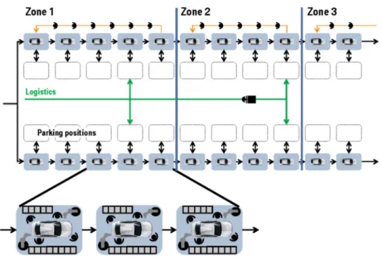
The flexible layout is designed to minimize the slowdowns caused by errors on the line. In the conventional layout, the band stops when a station encounters an error and only moves again once the error is resolved. Other stations in the band may become idle as a result. The slowdown propagates to the upstream band if the upstream buffer is full (i.e. blockage) and downstream band if the downstream buffer is empty (i.e. starvation). The flexible layout alleviates this issue by decoupling tasks from a
specific station. More specifically, cars are placed on mobile platforms that move in the band and carry all equipment necessary for all tasks in the band. When an error occurs, the platform has the flexibility to move into adjacent stations called parking stations. Cars behind the platform can move along the band without getting blocked. To the best of our knowledge, mobile platforms are not currently used in automotive assembly lines for the purpose of minimizing slowdowns caused by errors. Figure 2-3 shows an illustration of the flexible layout.
Figure 2-3: In the flexible layout, cars are placed on mobile platforms that move in a band or zone. The platforms carry all equipment necessary for the tasks in a band. The band has adjacent parking stations that platforms can move into if a platform requires more time to finish tasks or resolve errors. Note that buffers are not shown in this diagram. Courtesy of BMW.
We make the following assumptions in our model:
∙ Equipment for all tasks in the band are able to fit on a single platform.
∙ Agents are assigned to a single platform from the time the car enters the band until the time the car exits the band. Therefore, agents have to be able to execute all tasks in the band.
∙ We allow platforms to traverse the band even when no agents are assigned to them. The total number of agents in the conventional and flexible layout is fixed for fair throughput comparison. But more agents are assigned to a single platform in the flexible layout than a single station in the conventional layout, because the number of agents assigned to a single platform is the maximum number of agents required for a single task. In the conventional layout, the number of agents assigned to a station is the maximum number of agents re-quired for a single task at the station, instead of the whole band. Allowing idle platforms helps fill up the band; otherwise stations are under-utilized. The parking stations also serve as stations for platforms that require extra time to complete all tasks.
Many sections of the automotive assembly line don’t fit the assumptions listed above. In fact, we do not intend the flexible layout to replace the conventional layout for the entire assembly line. Instead, we envision a hybrid line that uses the flexible layout on bands that are bottlenecks due to higher frequency of errors.
A question that came up during the design of the flexible layout was whether the platforms move through the band if the tasks are decoupled from specific stations. In other words, since all tasks are done on a single platform, the platform can be a stationary workstation that processes all tasks for a single car. We chose to make the platforms mobile for the following reasons:
1. We want to keep the structure of the assembly line where there is a loading zone for cars to load onto a platform and an unloading zone for cars to exit the band and enter a buffer. If the platforms are stationary, there will be multiple loading and unloading zones for a given band.
2. The assumption that requires the platforms to carry all equipment may be infeasible. However, the flexible model can still be adopted by situating the bulkier or more expensive equipment in a few stations. This will add additional constraints for platforms to pass by specific stations for certain tasks, but it still allows platforms to move into parking stations if necessary to avoid propagation
of delays. A more rigorous analysis of such a model is an area for further research.
In Section 2.2.1, we provide definitions for our model, and in Section 2.2.2, we provide an overview of the algorithm.
2.2.1
Definitions
For definitions of task, car, and temporal constraints, refer to Section 2.1.1. Here, we define additional terms pertaining to the flexible layout as well as terms that differ from the conventional layout.
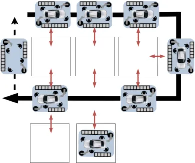
Figure 2-4: The flexible layout uses a sideways U-shaped band. The red arrows indicate the parking stations available to the platforms. The platforms load cars at the top and unload cars at the bottom. After unloading a car, the platform and the agents traverse back to the beginning of the band to load another car.
U Band
In the conventional layout, a linear band is described. For the simulation of the flexible layout, we consider a sideways U-shaped band where cars enter at the top of the U and exit at the bottom. This allows the platforms to access the same parking stations from multiple stations in the band. Once a platform unloads a finished car
to the next band, the agents and the platform travel back to the beginning of the band. A U-shaped band minimizes this travel time. Figure 2-4 illustrates this layout.
Station
We still divide the band into stations even though no tasks or agents are assigned to them. At most one platform can occupy a station at any given time.
Parking Station 𝑝𝑠
A parking station 𝑝𝑠 is a designated station for platforms to move to if the platform requires more time to finish tasks or resolve errors. Like stations in the band, a parking station can be occupied by at most one platform at a time. A platform can only move to parking stations that are adjacent to itself. We’re provided a function that given a station 𝑥 returns a set of adjacent parking stations 𝑃 𝑆, 𝑓 (𝑥) → 𝑃 𝑆.
Mobile Platform
A mobile platform moves a car in a band and carries all equipment necessary for all tasks in the band. The mobile platform is able to move to all adjacent stations (including parking stations) in a cycle. The agents may be standing on the platform or right next to the platform.
Agent 𝑎 < 𝑐𝑎 >
An agent 𝑎 is assigned to a car 𝑐𝑎, and the set of agents assigned to a car 𝑐 is denoted
by 𝐴𝑐. This is in contrast to the conventional layout, where agents are assigned to
specific stations.
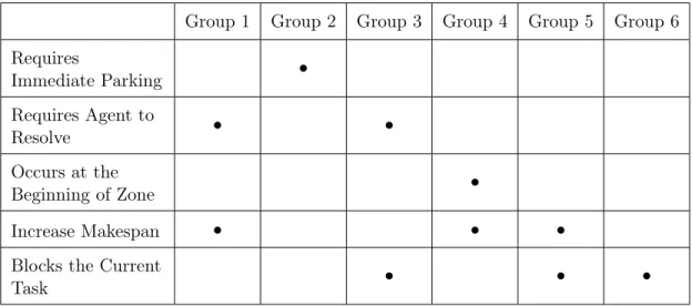
Error 𝑒 < 𝑑𝑒, 𝑔𝑒>
The error model used in the simulation of the flexible layout differs from that used in the conventional layout. An error 𝑒 is defined by the error duration 𝑑𝑒 and the group
The grouping of an error depends on the following properties:
Requires Immediate Parking: The platform has to park immediately and wait at the parking station until the error is resolved. If no parking station is available, the platform waits until a parking station becomes available; otherwise it stays in the error state.
Requires Agent to Resolve: One of the agents on the platform is assigned to resolve the error, and cannot perform tasks for the duration of the error. This type of error includes causes such as tool wear or machine breakdown. Errors that do not require an agent to resolve includes logistical delays.
Occurs at the Beginning of Band: The error can only occur at the first station where the car loads from a buffer onto a platform. This error is caused by failures or malfunctions in the transfer mechanism from buffer to a platform.
Increases Makespan: The error increases the makespan of the car due to any rework that has to be done.
Blocks the Current Task: The current task cannot be worked on until the error is resolved. Any progress on the task is lost.
Table 2.1 shows the error groups and their associated properties.
Group 1 Group 2 Group 3 Group 4 Group 5 Group 6 Requires Immediate Parking ∙ Requires Agent to Resolve ∙ ∙ Occurs at the Beginning of Zone ∙ Increase Makespan ∙ ∙ ∙
Blocks the Current
Task ∙ ∙ ∙
2.2.2
Algorithm
An overview of the flexible layout simulation is discussed in this section. More details can be found in [28].
Like the conventional layout simulation, the system is composed of a pre-processor, scheduler, and simulator. The pre-processor merges tasks with simultaneous and immediate constraints into single tasks to simplify task scheduling. The merging of tasks is the same as in the conventional case except that there are no restrictions for merging tasks in the same station. For the conventional layout, tasks assigned to different stations cannot be merged. This is no longer true because tasks are decoupled from stations in the flexible layout. The scheduler schedules tasks for each individual car 𝑐 by assigning start times 𝑠𝑡𝑤 and end times 𝑒𝑡𝑤 and agents for all 𝑤 ∈ 𝑊𝑐. The
scheduler also reschedules tasks if a car experiences an error that requires an agent to solve and/or blocks the current task. In the former case, the task the agent is working on is paused for the duration of the error. In the latter case, the progress on the current task is voided, and the task is rescheduled for some time after the error is resolved. Similar to the conventional simulation, the simulator keeps track of the band and cars as well as processing time events from a min-heap queue. Algorithm 2 shows the pseudocode for the simulator.
If a car cannot finish tasks or resolve errors before leaving the band, the simulator tries to move the car to a parking station. We use a greedy strategy for parking cars. Algorithm 3 shows the pseudocode for the parking algorithm. In lines 1-6, if an adjacent parking is available, the car is moved to the parking station. However, if no adjacent parking is available, lines 7-16 check if the cars in adjacent parking stations can move to other stations. Note that this algorithm is not optimal, and we discuss methods for improving the parking strategy in Chapter 4.
To summarize, the main differences between the conventional and flexible simula-tion are listed below:
∙ For the conventional layout, tasks with immediate constraints that are assigned to different stations cannot be merged. But in the flexible layout, all tasks are
Algorithm 2: Flexible Layout Simulator while less than n cars exited do
timeEvent ← queue.pop();
if timeEvent == Car Enters Band then assign agents to the car if possible; move car onto first station in band; schedule tasks for the car;
else if timeEvent == Car Exits Band then
check that car finished all tasks and is not in error state; remove car from last station in band;
the agents working on exited car become available; else if timeEvent == Error Occurs then
if Parking Required then
park(car); // see Algorithm 3 else if Rescheduling Required then
reschedule tasks;
update makespan of car; change car state to in error;
else if timeEvent == Error Resolved then change car state to not in error;
else if timeEvent == Cycle Ends then
if car at last station is ready to leave band then add Car Exits Band event to queue;
end
for Car c in band do
if car c cannot finish tasks or resolve errors before leaving band then
park(c); // see Algorithm 3 end
end
move cars along the band, allow cars to leave parking stations first; assign agents to idle platforms;
create time events for errors in next cycle and store events in queue; end
Algorithm 3: Parking Algorithm input: Car c
1 for parking station p accessible to car c do 2 if p is not occupied then
3 move car c to parking station p;
4 return;
5 end
6 end
7 for parking station p accessible to car c do 8 𝑐𝑝 ← car currently in parking station p; 9 if 𝑐𝑝 already moved this cycle then
10 continue;
11 end
12 for parking station q accessible to car 𝑐𝑝 do 13 if q is not occupied then
14 move car 𝑐𝑝 to parking station q; 15 move car c to parking station p;
16 return;
17 end
18 end
19 end
performed on a single platform and do not have that restriction.
∙ For the conventional layout, the scheduler schedules tasks for a single cycle which is then processed by the simulator until the cycle ends. The process then repeats until a fixed number of cars exits the band. For the flexible layout, the scheduler schedules all tasks for a single car when the car enters the band, and may reschedule tasks for a car if necessary.
2.2.3
Scheduling and Rescheduling
The scheduler works by greedily assigning tasks without delay constraints to agents. If there are more tasks than agents, tasks are chosen arbitrarily. The rest of the tasks are assigned when the delay constraints are satisfied. Pseudocode for the greedy scheduler is provided in Algorithm 4. In the conventional case, this process is done for all tasks in a single cycle while in the flexible case, this process is done for all tasks for a car.
Algorithm 4: Flexible Layout Greedy Scheduler 𝑢𝑛𝑠𝑐ℎ𝑒𝑑𝑢𝑙𝑒𝑑𝑇 𝑎𝑠𝑘𝑠 ← tasks for current car; 𝑐𝑜𝑛𝑠𝑡𝑟𝑎𝑖𝑛𝑡𝑠 ← constraints for 𝑢𝑛𝑠𝑐ℎ𝑒𝑑𝑢𝑙𝑒𝑑𝑇 𝑎𝑠𝑘𝑠;
𝑎𝑣𝑎𝑖𝑙𝑎𝑏𝑙𝑒𝑇 𝑎𝑠𝑘𝑠 ← 𝑢𝑛𝑠𝑐ℎ𝑒𝑑𝑢𝑙𝑒𝑑𝑇 𝑎𝑠𝑘𝑠 without constraints; // set of agents assigned to car 𝑐
𝑎𝑣𝑎𝑖𝑙𝑎𝑏𝑙𝑒𝐴𝑔𝑒𝑛𝑡𝑠 ← 𝐴𝑐 ;
Initialize 𝑞𝑢𝑒𝑢𝑒 as empty min-heap; assign agents to 𝑎𝑣𝑎𝑖𝑙𝑎𝑏𝑙𝑒𝑇 𝑎𝑠𝑘𝑠;
insert task completed events with completion time to 𝑞𝑢𝑒𝑢𝑒; while not all tasks assigned do
timeEvent ← queue.pop();
if timeEvent == Task 𝑤 Completed then for all tasks with 𝑤 as delay constraint do
insert delay constraint satisfied events at current time + delay time to 𝑞𝑢𝑒𝑢𝑒;
end
agents ← agents that worked on task 𝑤; 𝑎𝑣𝑎𝑖𝑙𝑎𝑏𝑙𝑒𝐴𝑔𝑒𝑛𝑡𝑠.add(agents);
else if timeEvent == Delay Constraint Satisfied then if no constraints on task then
𝑎𝑣𝑎𝑖𝑙𝑎𝑏𝑙𝑒𝑇 𝑎𝑠𝑘𝑠.add(task); end
if availableTasks is not empty then assign agents to tasks;
end end
Because the schedule for all tasks is determined when a car enters the band, when an error occurs that disrupts the current task, the schedule is no longer valid. We describe the rescheduling algorithm for two error cases: 1. requires an agent to resolve and 2. blocks the current task.
Requires Agent to Resolve
This error requires an agent to resolve, which makes the agent unavailable for the duration of the error. The task the agent was working on can be picked up again by the same agent after the error is resolved or by another agent. Tasks that have been completed before the error occurs have the same schedule, while the rest of the tasks are rescheduled. The greedy algorithm is applied to the set of tasks that require rescheduling, which is then appended to the schedule for the tasks that have completed.
Algorithm 5: Flexible Layout Rescheduling Algorithm
𝑢𝑛𝑠𝑐ℎ𝑒𝑑𝑢𝑙𝑒𝑑𝑇 𝑎𝑠𝑘𝑠 ← tasks that haven’t been executed at the time the error occurred;
For all other tasks in progress, create new tasks with duration = task time left and add to 𝑢𝑛𝑠𝑐ℎ𝑒𝑑𝑢𝑙𝑒𝑑𝑇 𝑎𝑠𝑘𝑠; // if error blocks the current task, one of the tasks loses progress
𝑐𝑜𝑛𝑠𝑡𝑟𝑎𝑖𝑛𝑡𝑠 ← delay constraints for 𝑢𝑛𝑠𝑐ℎ𝑒𝑑𝑢𝑙𝑒𝑑𝑇 𝑎𝑠𝑘𝑠; if error blocks the current task then
𝑑𝑒𝑙𝑎𝑦𝐶𝑜𝑛𝑠𝑡𝑟𝑎𝑖𝑛𝑡 ← constraint on task with delay = error duration; // create delay constraint that prevents task 𝑡 from being worked on until after error is resolved
add 𝑑𝑒𝑙𝑎𝑦𝐶𝑜𝑛𝑠𝑡𝑟𝑎𝑖𝑛𝑡 to 𝑐𝑜𝑛𝑠𝑡𝑟𝑎𝑖𝑛𝑡𝑠;
any progress on task 𝑡 is lost; therefore add 𝑡 to 𝑢𝑛𝑠𝑐ℎ𝑒𝑑𝑢𝑙𝑒𝑑𝑇 𝑎𝑠𝑘𝑠; 𝑎𝑣𝑎𝑖𝑙𝑎𝑏𝑙𝑒𝐴𝑔𝑒𝑛𝑡𝑠 ← 𝐴𝑠;
end
if error requires an agent to solve then
pick agent 𝑎 to resolve error; // agent can be picked arbitrarily or pick an agent that has made the least progress on a task 𝑎𝑣𝑎𝑖𝑙𝑎𝑏𝑙𝑒𝐴𝑔𝑒𝑛𝑡𝑠 ← 𝐴𝑠∖ 𝑎; // available agents are all agents
assigned to current car 𝐴𝑠 minus agent 𝑎 who is resolving
error end
Run greedy scheduler algorithm;
This error stops the task, and all progress on the task is lost. The original task is added back to the list of unscheduled tasks. A delay constraint with delay time equal to the error duration is added so that the task cannot be scheduled until after the error is resolved. Algorithm 5 shows the pseudocode for the rescheduling algorithms.
2.3
Multi-Band Simulation
The multi-band simulation is a natural extension for the comparison of the conven-tional and flexible layouts. We consider two bands with a single finite buffer. Buffers are used in many production systems as inventory storage when the systems have unreliable machines . Without buffers, if a band is down due to an error, the whole line is forced down. We use forced down to describe a band that becomes idle due to errors in neighboring bands. Buffers allow other bands to continue work when a single band fails. However, a band in a system with buffers can still be forced down if the upstream buffer is empty (i.e. starvation) or if the downstream buffer is full (i.e. blockage). The optimal design of buffer location and sizes, also known as the buffer allocation problem, is a challenging problem and is an active area of research [12]. Here, we’re interested in the throughput comparison of the conventional and flexible layouts with different buffer sizes.
2.3.1
Definitions
We define a two-band model with a finite buffer as well as provide notations for larger models. For a two-band model, let 𝑀𝑢 be the upstream band and 𝑀𝑑 be the
downstream band. The buffer is denoted by 𝐵 < 𝑐𝑏, 𝑙𝑏 >, with parameters capacity 𝑐𝑏
which is the number of cars the buffer can hold and 𝑙𝑏 which is the current inventory
level of the buffer. If 𝐵 is full, 𝑀𝑢 is blocked, and if 𝐵 is empty, 𝑀𝑑 is starved.
For a line with 𝑛 bands, let 𝑀𝑖, 𝑖 ∈ 1...𝑛, denote the bands. Then, there exists
𝑛 − 1 buffers denoted by 𝐵𝑖, 𝑖 ∈ 1...𝑛 − 1. 𝑀1 is connected to 𝐵1, which is connected
to 𝑀1, which is connected to 𝐵1, and so on until 𝐵𝑛−1 is connected to 𝑀𝑛.
∙ In a two-band model, 𝑀𝑢 is never starved, and 𝑀𝑑is never blocked. For longer
lines, 𝑀0 is never starved, and 𝑀𝑛 is never blocked.
∙ Because of DES, the buffer state only changes at the end of cycles. At the end of 𝑀𝑢’s cycle, the inventory level of the buffer increases by one if it’s not full.
At the end of 𝑀𝑑’s cycle, if the buffer is not empty and 𝑀𝑑can load a new car,
the inventory level of the buffer decreases by one.
∙ The buffer has no transition time. Once a car loads onto the buffer, it can immediately load onto the downstream band.
∙ For the conventional layout, 𝑀𝑢 always produces a car and 𝑀𝑑 always loads a
car at the end of a cycle. The band stops when resolving an error, and thus increases the cycle time. But after the cycle, all cars move to the next positions. For the flexible layout, the cycle time is fixed, so a car only enters or exits a band at the end of the fixed cycles.
2.3.2
Algorithm
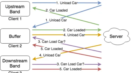
At the time of writing the thesis, data are only available for a single band. Therefore, we approximate the performance of a two-band line by replicating the tasks for a single band. To extend single band simulation to multiple bands, we use a client-server model to pass messages between the upstream band, downstream band, and the buffer. The bands and the buffer are clients that send messages to the server, which then relays the messages to their intended receivers. The upstream band and downstream band only communicate with the buffer, and the buffer communicates with both bands.
When the upstream band is ready to unload a car (i.e. car is ready to exit), the band sends a message to the buffer. If the buffer is not full, it replies to the band immediately, and increases its inventory level by one. However, if the buffer is full, it waits until a spot is open to reply back. In the conventional layout, the upstream band is blocked until the buffer replies back. In the flexible layout, the upstream
Figure 2-5: We use a client-server model to relay messages for loading and unloading cars. Each colors denotes a single message. 1. The upstream band sends a message to the buffer when a car is ready to exit. 2. If the buffer is not full, it replies to the upstream band that the car is loaded. 3. The downstream band sends a message to the buffer when a car can enter the band. 4. If the buffer is not empty, it replies to the downstream band that a car is ready to unload from the buffer. 5. Downstream band acknowledges to the buffer that it has received the car.
band may be able to load a new car by moving cars into parking stations. It only becomes blocked when all stations in band and parking stations are occupied. On the other hand, when the downstream band is ready to load a car, the band sends a message to the buffer. The buffer immediately replies back with a message indicating if it’s empty or if the band can load a car. The downstream band continues to the next cycle in either situation. Only when the entire downstream band is empty will it be starved.
2.4
Experiments
This section describes the experimental design for comparing the throughput of con-ventional and flexible layouts. In Section 2.4.1, we discuss the dataset used in the simulations. In Section 2.4.2, we discuss some decisions made to make the comparison as fair as possible.
(a) The upstream band is ready to unload a car onto the buffer. It sends a message to the buffer, but the buffer does not reply back until it can load a car.
(b) The downstream band can load a car. It sends a message to the buffer, but the buffer replies that it is empty. The down-stream band continues to the next cycle if it is not empty.
Figure 2-6
2.4.1
Dataset
The dataset for tasks and errors are based on a single band in a BMW automotive assembly line. The cars produced are highly customizable, which means that the tasks vary between cars. We’re provided a blackbox tool that generates sets of tasks and constraints, taking into account frequencies of different customization. As reported in [28], the tool takes 8 minutes to generate tasks for one car in a virtual machine on a commercial 2.3GHz Intel Core i5 processor with 8GB of RAM. To speed up the simulation, we uniformly sample from a pre-generated pool of 1, 385 car variants. We’re also provided a blackbox tool that samples error group and duration from some probability distribution for both conventional and flexible layouts. The errors used in the simulation are uniformly sampled from a pre-generated pool of 1, 194 errors for each layout.
For each cycle, each station that is working on tasks (in the conventional layout) or that is occupied by a platform (in the flexible layout), has a probability 𝑝 of
experiencing an error. The parameter 𝑝 is chosen such that the expected number of errors is equal to the number of errors observed in a real factory. We’re also interested in evaluating the layouts with different probabilities of error. More specifically, we used different multiples of 𝑝, {0, 0.25, 0.5, 1, 2, 4, 8}, in the simulation.
Each simulation is run until 700 cars are produced, which is the daily production rate of the factory our model is based on. For each error multiple, 30 simulations are run. In both layouts, we use a cycle time of 100 seconds.
2.4.2
Comparison Design
Agents and Stations: In the conventional layout, the number of agents at each station is chosen such that there are enough agents to perform any single task assigned to the station. In the flexible layout, the number of agents assigned to each platform is the maximum number of agents required to perform a single task. For optimal throughput, the number of agents required is the maximum number of agents for a platform multiplied by the number of stations in the band. However, we chose to use the same number of agents in the conventional and flexible layouts to make the comparison fair.
Band Layout: We use the same band layouts as reported in [28]. The conven-tional layout is a linear band while the flexible layout is a sideways U-shaped band. Based on factory measurements, the conventional layout has 14 stations, each station being 6.65 meters long. [28] reported that if both layouts have the same band length, the flexible layout would have low agent utilization (i.e. agent idle time is high). Be-cause of the lack of spacial constraints in the flexible layout, tasks are finished faster than in the conventional layout. To reduce agent idle time, the authors of [28] used a band length of 60 meters or 9 stations, which we also use in our simulation.
2.5
Results & Discussion
We evaluate the performance of the conventional and flexible layouts by the number of cars produced per hour. Each simulation is run until 700 cars are produced, and
the results are averaged over 30 simulations. We show that the flexible layout achieves an average 25.6% speed up for the single band case and an average 35.9% speed up for the two-band case with a buffer size of 10. Section 2.5.1 discusses results for the single band case, and Section 2.5.2 discusses results for the two-band case.
2.5.1
Single Band
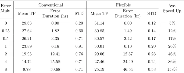
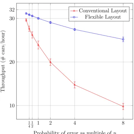
Table 2.2 and Figure 2-7 show the average throughput for different error multiples in numerical and graphical formats respectively. For factory-observed error probability, which has an error multiple of 1, the conventional layout has a production rate of 23.89 units/hour while the flexible layout has 30.01 units/hour. The flexible layout achieves an average 25.6% speed up over the conventional layout.
Error Mult.
Conventional Flexible Ave.
Speed Up Mean TP Error Duration (hr) STD Mean TP Error Duration (hr) STD 0 29.63 0.00 0.29 31.14 0.00 0.12 5% 0.25 27.64 1.82 0.60 30.85 1.49 0.14 12% 0.5 26.21 3.35 0.71 30.57 3.42 0.17 17% 1 23.89 6.16 0.91 30.01 6.10 0.20 26% 2 19.95 12.41 0.76 29.06 12.57 0.23 46% 4 14.74 25.58 0.71 27.46 24.49 0.24 86% 8 9.78 50.68 0.71 25.19 46.54 0.53 158%
Table 2.2: Comparison of conventional and flexible layout simulation results. TP is the throughput in units produced per hour, and STD is the standard deviation of TP. The error multiple is the multiple of 𝑝 (i.e. the probability of an error for a car in a cycle) used in the simulation, where 𝑝 is derived from our dataset.
Remark 1: When the line has no errors, the flexible layout has a slightly higher throughput than the conventional layout because of the lack of spacial constraints in the flexible layout. Since all tasks are performed on a single mobile platform, tasks can begin execution immediately after their temporal constraints are satisfied. In the conventional layout, the tasks may be assigned to different stations and can’t begin execution until the car is in a particular station.
Remark 2: The advantage of the flexible layout is more apparent as the frequency of error increases. Recall that when an error occurs on the conventional layout, the entire band stops until the error is resolved. Whereas in the flexible layout, the mobile platform moves to a parking station to resolve the error, and platforms upstream can continue down the line. Notice that the flexible layout throughput is similar for error multiples 0 to 2 and decreases more rapidly thereafter. This shows that the parking stations help mitigate error slowdowns up to a certain error frequency. Once the parking stations are all occupied, errors have the same effect as in the conventional layout.
In Table 2.2, the error duration is the total number of hours a station or platform spent on resolving an error. Note that it is not the absolute time the entire band was down. Since multiple stations or platforms can be down at the same time, the total error duration is the sum of all down times for all stations or platforms. The error duration is different for the conventional and flexible layouts since the errors are drawn from different distributions.
2.5.2
Two-Band
Before showing the simulation results, we define some properties of flow lines that are useful to the analysis [10]:
Monotonicity: The production rate monotonically increases as a function of the buffer capacities. More formally, consider two lines 𝐿1 and 𝐿2 with buffer capacities
𝑧1 and 𝑧2. If 𝑧1 ≤ 𝑧2, then 𝑇 𝑃 (𝐿1) ≤ 𝑇 𝑃 (𝐿2), where 𝑇 𝑃 (𝐿𝑖) is the throughput of
line 𝑖.
Infinite buffer size: For a line with infinite buffer capacity, the throughput of the line is bounded by the smallest throughput of an individual machine on the line. Reversibility: If a n-machine line is reversed such that machine 𝑀𝑖 in the original
line is the same as machine 𝑀𝑛−𝑖+1 in the reversed line, then the two lines have the
same production rate.
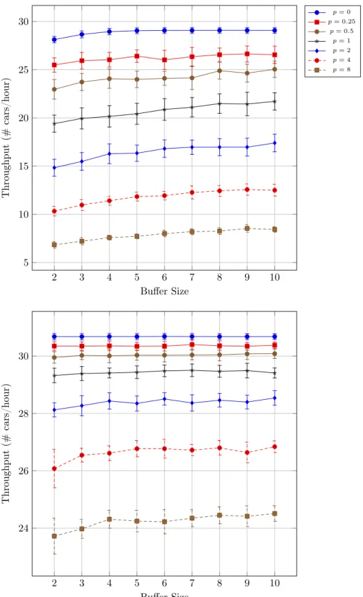
Figure 2-8 shows the throughput in units/hour for different error multiples and buffer sizes. Here, the error is the same for the upstream and downstream bands.
1 4 1 2 1 2 4 8 10 20 30 32
Probability of error as multiple of 𝑝
Throughput
(#
cars/hour)
Conventional Layout Flexible Layout
Figure 2-7: Throughput comparison
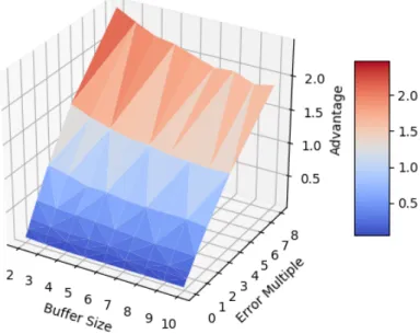
Remark 1: In most cases, the mean throughput follows the monotocity property. In cases that don’t, the throughput values that would make the property hold are within one standard deviation of the mean. Another important observation is that the throughput seems to converge, and that the maximum throughput is bounded by, or lower than, the throughput of the single band layout with the same error multiple. Figure 2-9 shows the advantage of the flexible layout over the conventional layout as a function of buffer size and error frequency. Table 2.3 shows the same data in numerical values. The advantage is calculated by
𝐴𝑑𝑣𝑎𝑛𝑡𝑎𝑔𝑒 = 𝑇 𝑃𝑓 𝑙𝑒𝑥𝑖𝑏𝑙𝑒− 𝑇 𝑃𝑐𝑜𝑛𝑣𝑒𝑛𝑡𝑖𝑜𝑛𝑎𝑙 𝑇 𝑃𝑐𝑜𝑛𝑣𝑒𝑛𝑡𝑖𝑜𝑛𝑎𝑙
where 𝑇 𝑃 is the throughput.
Remark 2: The flexible layout has the greatest advantage when the error multi-ples are high and the buffer size is small. As the buffer size increases, the advantage
2 3 4 5 6 7 8 9 10 5 10 15 20 25 30 Buffer Size Throughput (# cars/hour) 𝑝 = 0 𝑝 = 0.25 𝑝 = 0.5 𝑝 = 1 𝑝 = 2 𝑝 = 4 𝑝 = 8 2 3 4 5 6 7 8 9 10 24 26 28 30 Buffer Size Throughput (# cars/hour)
Figure 2-8: Throughput of the two-band conventional layout (top) and flexible layout (bottom) with equal band failure probability. The bars show the standard deviation of 30 simulation runs.
Figure 2-9: Advantage of the flexible layout over the conventional layout as a function of buffer size and error frequency. The upstream and downstream bands have the same error frequency. Error Multiple Buffer Size 0 0.25 0.5 1 2 4 8 2 0.091 0.188 0.305 0.511 0.895 1.537 2.473 3 0.07 0.169 0.266 0.474 0.827 1.412 2.323 4 0.06 0.167 0.249 0.459 0.741 1.323 2.185 5 0.056 0.15 0.253 0.442 0.736 1.254 2.138 6 0.056 0.167 0.245 0.412 0.691 1.235 2.032 7 0.055 0.152 0.241 0.395 0.676 1.17 1.937 8 0.055 0.143 0.206 0.371 0.676 1.156 1.953 9 0.055 0.14 0.219 0.374 0.677 1.129 1.837 10 0.055 0.144 0.2 0.359 0.636 1.141 1.891
decreases. This is because the buffer helps alleviate error propagation and has greater effect on a line that is more affected by errors. For factory-observed error probability, the two-band flexible layout has a 35.9% advantage over the conventional layout with buffer size of 10. For a line with no errors, the advantage stays at 5.5% for buffer sizes equal to or greater than seven. In this case, the throughput converged to its upper bound and increasing the buffer size does not improve the the throughput of either layouts. We expect the same behavior for lines with errors but for a much larger buffer size.
Figure 2-10: Throughput of conventional and flexible layouts with buffer size = 5.
We now fix the buffer size and consider the throughput of the line when the error frequencies are different for the upstream and downstream bands. Figure 2-10 shows the throughput as a function of error frequencies for the upstream and downstream bands. Both layouts have buffer size equal to five. Table 2.4 shows the same data in numerical values.
Upstream Band Error Multiple 0 0.25 0.5 1 2 4 8 Do wnstream Band Error Mult. 0 29.044 (0.31) 27.486 (0.58) 25.964 (0.76) 23.516 (0.76) 19.392 (1.00) 14.583 (0.63) 9.561 (0.34) 0.25 27.506 (0.73) 26.410 (0.65) 25.144 (1.00) 23.027 (1.00) 19.212 (0.88) 14.512 (0.74) 9.571 (0.45) 0.5 26.297 (0.78) 25.178 (0.79) 23.996 (0.86) 22.472 (0.93) 18.613 (1.02) 14.279 (0.68) 9.587 (0.45) 1 23.611 (0.87) 22.891 (1.01) 22.419 (0.85) 20.427 (1.09) 18.116 (0.80) 14.033 (0.65) 9.522 (0.35) 2 19.854 (0.84) 19.330 (0.75) 18.932 (0.81) 18.142 (0.98) 16.344 (0.84) 13.530 (0.66) 9.390 (0.37) 4 14.777 (0.73) 14.582 (0.72) 14.284 (0.59) 14.068 (0.56) 13.202 (0.73) 11.838 (0.47) 8.975 (0.50) 8 9.620 (0.38) 9.739 (0.45) 9.750 (0.40) 9.644 (0.39) 9.351 (0.42) 8.976 (0.41) 7.718 (0.25)
(a) Conventional Layout
Upstream Band Error Multiple
0 0.25 0.5 1 2 4 8 Do wnstream Band Error Mult. 0 30.680 (0.11) 30.354 (0.12) 30.095 (0.17) 29.449 (0.21) 28.487 (0.28) 26.892 (0.36) 24.647 (0.31) 0.25 30.638 (0.11) 30.375 (0.17) 30.074 (0.21) 29.467 (0.24) 28.565 (0.29) 26.944 (0.28) 24.598 (0.35) 0.5 30.526 (0.14) 30.299 (0.18) 30.065 (0.22) 29.539 (0.22) 28.559 (0.32) 26.824 (0.32) 24.514 (0.33) 1 30.094 (0.20) 29.950 (0.21) 29.847 (0.21) 29.449 (0.22) 28.628 (0.25) 26.928 (0.37) 24.705 (0.33) 2 29.121 (0.24) 29.036 (0.28) 29.089 (0.26) 28.906 (0.29) 28.369 (0.29) 26.843 (0.33) 24.726 (0.34) 4 27.455 (0.30) 27.476 (0.25) 27.542 (0.29) 27.422 (0.31) 27.390 (0.37) 26.685 (0.28) 24.564 (0.30) 8 25.087 (0.31) 25.104 (0.37) 25.156 (0.53) 25.072 (0.46) 24.751 (1.67) 25.063 (0.24) 24.223 (0.24) (b) Flexible Layout
Table 2.4: Throughput (standard deviation) of conventional and flexible layouts with buffer size = 5.
the upstream band has failure probability 𝑝1 and the downstream band has failure
probability 𝑝2 has the same throughput as a line where the upstream band has failure
probability 𝑝2 and the downstream band has failure probability 𝑝1. We also observe
that the throughput is higher for a line with both bands having an error multiple of 2 than a line with one band having no error and the other having an error multiple of 4. This follows the property that the efficiency of the whole line is bounded by the machine with the worst efficiency.
2.5.3
Limitations
Some of the limitations of the simulation include:
∙ We only modeled a subset of errors observed in a real factory. For the conven-tional layout, we abstracted errors into one category. For the flexible layout, we grouped errors into a few categories but not all types of errors are consid-ered. This is due to the data collection and the complexities of error types. For example, power line failures that affect multiple stations are more complex to model.
∙ The deployment of mobile platforms may incur additional inefficiencies in the production process. For example, agents have to be trained on all tasks for the band instead of just a few tasks at a single station. We do not know the effect of an increase in task variety on productivity, if there is any. Another possible inefficiency is the speed of the mobile platforms which may differ from the speed of the band in the conventional layout.
Despite the limitations, the simulation provides a tool for evaluating throughput performance and serves as a metric for the adoption of the flexible layout. In this chapter, we discussed using discrete event simulation to model the automotive assem-bly line and showed that the flexible layout has significant advantage in throughput over the conventional layout. In the next chapter, we present analytical models of the conventional and flexible layouts.
Chapter 3
Analytical Models of Automotive
Assembly Line
Analytical models are important for the design and throughput analyses of assembly lines. Because simulation models take a long time to implement, require large com-putational resources, and are prone to bugs, analytical models are often used first to assess the performance of a design. However, they have their own challenges and are also only used as approximations to the analysis of a real assembly line. One of the main challenges is that exact analytical methods only exist for two-machine line models due to the large state space of assembly line systems. To date, the main approach for estimating the performance of longer lines is to use two-machine models as building blocks [30]. In addition to large state spaces, choosing the right model is important because of the variety of real world assembly line systems. Also, model-ing a system with real world data has proved to be challengmodel-ing. In [6], the authors evaluated several two-machine line models and found that the difference between an-alytical and simulation models based on real factory data is significant. Having built simulations for our conventional and flexible layouts, we’re interested in developing accurate analytical models as well as compare the analytical and simulation results.
In this chapter, we evaluate previous models that match the assumptions of our system as well as develop our own analytical models for throughput analyses. We consider both single band and two-band models and compare their results to our
simulation models from Chapter 1. We show that we can use analytical models to estimate the throughput of the conventional and flexible layouts with less than 11% and 18% error respectively. In this chapter, we use machines to refer to stations in the conventional layout or platforms in the flexible layout. The cars that enter the band will be referred to as a part or inventory. A machine failure is used as a general term to describe all possible errors modeled in our system.
In Section 3.1, we provide definitions of terms used to categorize assembly line systems. In Section 3.2, we provide an overview of the analytical models discussed in this chapter and list their assumptions. We present the single band analytical models in Section 3.3 and the two-band analytical models in Section 3.4. We discuss parameter estimation in Section 3.5 and present the results in Section 3.6.
3.1
Definitions
Many analytical models exist due to the variety of real world assembly line systems. Here, we define terms that are used to categorize them and provide more details about our models. A more comprehensive list of definitions can be found in [10].
Assembly Line
In most literature, assembly lines are generalized as flow line systems where a line is composed of machines separated by buffers. Flow lines can refer to systems that handle discrete entities such as car parts or continuous material such as fluids. For systems that handle discrete entities, time is usually discretized into cycles, which is the amount of time a part spends at a machine. The line is separated by buffers whose main purpose is to decouple machines. Buffers can be placed between every machine or series of machines. The class of flow lines that have stochastic failures is known as flow lines with unreliable machines (FLUM), while the class of flow lines with no failures is known as flow lines with reliable machines (FLRM). Most mass production systems are modeled as FLUM with deterministic service times and finite buffers [30]. Our models fall in this category, except that they have stochastic service
times due to the variety of parts produced on the line.
Failures and Repairs
Let the line be composed of 𝑛 machines. Each machine 𝑀𝑖 for 𝑖 ∈ 𝑛 has a probability
𝑝𝑖 of breaking down in each cycle. Once the machine is down, the average number
of cycles it takes to repair machine 𝑀𝑖 is denoted as 𝑀 𝑇 𝑇 𝑅𝑖, or the mean time to
repair (unit of time is a cycle). The average time for machine 𝑀𝑖 to fail is denoted
as 𝑀 𝑇 𝑇 𝐹𝑖, or the mean time to failure. 𝑀 𝑇 𝑇 𝑅 is also referred to as the mean down
time, and 𝑀 𝑇 𝑇 𝐹 is also referred to as the mean operational time or mean up time. Let 𝑟𝑖 be the probability that machine 𝑀𝑖 is repaired in a cycle given that it is down
at the beginning of the cycle.
𝑟𝑖 = 1 𝑀 𝑇 𝑇 𝑅𝑖 (3.1) 𝑝𝑖 = 1 𝑀 𝑇 𝑇 𝐹𝑖
Here, the uptime (𝑀 𝑇 𝑇 𝐹 ) and downtime (𝑀 𝑇 𝑇 𝑅) of machines follow geometric distributions. This type of model is also referred to as a discrete model because the time unit is discretized into cycles. For a continuous model, the uptime and downtime of machines follow exponential distributions. We use 𝜆𝑖 and 𝜇𝑖 to represent the failure
rate and repair rate of the 𝑖𝑡ℎ machine. Equation 3.1 becomes
𝜇𝑖 = 1 𝑀 𝑇 𝑇 𝑅𝑖 (3.2) 𝜆𝑖 = 1 𝑀 𝑇 𝑇 𝐹𝑖
Failures can be divided into two categories: time-dependent or operation-dependent. A time-dependent failure (TDF) can occur anytime while an operation-dependent failure (ODF) only occurs when a machine is operating. Some examples of TDF include power line or transfer mechanism failures, while ODF are related to tasks and include equipment breakdown or logistical delays. [6] recorded the failures of two