Measurements of top-quark pair spin correlations in the $e\mu$ channel at $\sqrt{s} = 13$ TeV using $pp$ collisions in the ATLAS detector

(1)

EUROPEAN ORGANISATION FOR NUCLEAR RESEARCH (CERN)

Eur. Phys. J. C 80 (2020) 754

DOI:10.1140/epjc/s10052-020-8181-6

CERN-EP-2019-034 11th November 2020

Measurements of top-quark pair spin correlations

in the 𝒆 𝝁 channel at

√

𝒔 = 13 TeV using 𝒑 𝒑

collisions in the ATLAS detector

The ATLAS Collaboration

A measurement of observables sensitive to spin correlations in 𝑡 ¯𝑡 production is presented, using 36.1 fb−1of 𝑝 𝑝 collision data at

√

𝑠 = 13 TeV recorded with the ATLAS detector at the Large Hadron Collider. Differential cross-sections are measured in events with exactly one electron and one muon with opposite-sign electric charge as a function of the azimuthal opening angle and the absolute difference in pseudorapidity between the electron and muon candidates in the laboratory frame. The azimuthal opening angle is also measured as a function of the invariant mass of the 𝑡 ¯𝑡 system. The measured differential cross-sections are compared to predictions by several NLO Monte Carlo generators and fixed-order calculations. The observed degree of spin correlation is somewhat higher than predicted by the generators used. The data are consistent with the prediction of one of the fixed-order calculations at NLO, but agree less well with higher-order predictions. Using these leptonic observables, a search is performed for pair production of supersymmetric top squarks decaying into Standard Model top quarks and light neutralinos. Top squark masses between 170 and 230 GeV are largely excluded at the 95% confidence level for kinematically allowed values of the neutralino mass.

Reproduction of this article or parts of it is allowed as specified in the CC-BY-4.0 license.

(2)

1 Introduction

The lifetime of the top quark is shorter than the timescale for hadronisation (∼10−23s) and is much shorter than the spin decorrelation time (∼10−21s) [1]. As a result, the spin information of the top quark is transferred directly to its decay products. Top quark pair production (𝑡 ¯𝑡) in QCD is parity invariant and hence the top quarks are not expected to be polarised in the Standard Model (SM); however, the spins of the top and the anti-top quarks are predicted to be correlated. This correlation has been observed experimentally by the ATLAS and CMS collaborations in proton–proton collision data at the Large Hadron Collider (LHC) at centre-of-mass energies of

√

𝑠= 7 TeV [₂_–₅_{] and} √

𝑠= 8 TeV [₆_–₉_{]. It has been also} studied in proton–antiproton collisions at the Tevatron collider [10–14]. This paper presents measurements of spin correlation at a centre-of-mass energy of

√

𝑠= 13 TeV in proton–proton collisions using the ATLAS detector and data collected in 2015 and 2016.

Due to the unstable nature of top quarks, their spin information is accessed through their decay products. However, not all decay particles carry the spin information to the same degree, with charged leptons arising from leptonically decaying 𝑊 bosons carrying almost the full spin information of the parent top quark [15–18]. This feature, along with the fact that charged leptons are readily identified and reconstructed by collider experiments, means that observables to study spin correlation in 𝑡 ¯𝑡 events are often based on the angular distributions of the charged leptons in events where both 𝑊 bosons decay leptonically (referred to as the dilepton channel). The simplest observable is the absolute azimuthal opening angle between the two charged leptons [19], measured in the laboratory frame in the plane transverse to the beam line. This opening angle is denoted by Δ𝜙. Non-vanishing spin correlation was observed by the ATLAS experiment using the Δ𝜙 observable and

√

𝑠= 7 TeV data [₂_{]. Since that time, spin correlation in 𝑡 ¯𝑡 pairs has been} extensively studied by both ATLAS and CMS using many observables and techniques. Spin correlation measurements have also been used to search for physics beyond the Standard Model (BSM) either directly, by searching for decreases in the expected SM spin correlation induced by scalar supersymmetric top squarks (stops) [6], or indirectly by setting limits on effective field theory operators, such as the chromo-magnetic and chromo-electric dipole operators [8]. Previous measurements by ATLAS [2,3,6] and CMS [5,8] using Δ𝜙 show slightly stronger spin correlation than expected in the SM, but with experimental uncertainties large enough that the results are still consistent with the SM expectation. In this paper, improved Monte Carlo (MC) generators are employed relative to previous spin correlation results from ATLAS to better control the systematic uncertainties. The spin correlation is measured as a function of the invariant mass of the 𝑡 ¯𝑡 system, as well as inclusively.

Charged-lepton observables can be used to search for the production of supersymmetric top squarks with masses close to that of the SM top quark. Such a scenario is difficult to constrain with conventional searches; however, observables such as Δ𝜙 and the absolute difference between the pseudorapidities of the two charged leptons, Δ𝜂, are highly sensitive in this regard. The Δ𝜙 distribution was previously used in such a search by ATLAS [6] and this new paper also includes Δ𝜂 for this purpose. Although this observable is only mildly sensitive to the SM spin correlation, it is sensitive to different supersymmetry (SUSY) hypotheses; the two observables are therefore used together in this paper to set limits on SUSY top squark production.

This paper is organised as follows. The ATLAS detector is described in Section 2. Section 3 describes the data and Monte Carlo (MC) used in the analysis and Section 4 describes the object definitions and event selection requirements. The unfolding procedure is described in Section 5 and the systematic uncertainties that are considered are described in Section 6. The differential cross-section results are presented in Section

(4)

7, the spin correlation extraction is described in Section 8, and the SUSY limits are presented in Section 9. Finally, the conclusions of the paper are summarised in Section 10.

2 ATLAS detector

The ATLAS detector [20] at the LHC covers nearly the entire solid angle1around the interaction point. It consists of an inner tracking detector surrounded by a thin superconducting solenoid, electromagnetic and hadronic calorimeters, and a muon spectrometer incorporating three large superconducting toroidal magnet systems. The inner-detector system is immersed in a 2 T axial magnetic field and provides charged-particle tracking in the range |𝜂| < 2.5.

The high-granularity silicon pixel detector surrounds the collision region and provides four measurements per track. The innermost layer, known as the insertable B-Layer [21,22], was added in 2014 and provides high-resolution hits at small radius to improve the tracking performance. The pixel detector is followed by the silicon microstrip tracker, which provides four three-dimensional measurement points per track. These silicon detectors are complemented by the transition radiation tracker, which enables radially extended track reconstruction up to |𝜂| = 2.0. The transition radiation tracker also provides electron identification information based on the number of hits (typically 30 in total) passing a higher charge threshold indicative of transition radiation.

The calorimeter system covers the pseudorapidity range |𝜂| < 4.9. Within the region |𝜂| < 3.2, electromagnetic calorimetry is provided by barrel and endcap high-granularity lead/liquid-argon (LAr) sampling calorimeters, with an additional thin LAr presampler covering |𝜂| < 1.8 to correct for energy loss in material upstream of the calorimeters. Hadronic calorimetry is provided by the steel/scintillator-tile calorimeter, segmented into three barrel structures within |𝜂| < 1.7, and two copper/LAr hadronic endcap calorimeters that cover 1.5 < |𝜂| < 3.2. The solid angle coverage is completed with forward copper/LAr and tungsten/LAr calorimeter modules optimised for electromagnetic and hadronic measurements respectively, in the region 3.1 < |𝜂| < 4.9.

The muon spectrometer comprises separate trigger and high-precision tracking chambers measuring the deflection of muons in a magnetic field generated by superconducting air-core toroids. The precision chamber system covers the region |𝜂| < 2.7 with three layers of monitored drift tubes, complemented by cathode strip chambers in the forward region, where the background is highest. The muon trigger system covers the range |𝜂| < 2.4 with resistive-plate chambers in the barrel, and thin-gap chambers in the endcap regions.

A two-level trigger system is used to select interesting events [23]. The level-1 trigger is hardware-based and uses a subset of detector information to reduce the event rate to a design value of at most 100 kHz. This is followed by the software-based high-level trigger, which reduces the event rate to around 1 kHz.

1_{ATLAS uses a right-handed coordinate system with its origin at the nominal interaction point (IP) in the centre of the detector}

and the 𝑧-axis along the beam pipe. The 𝑥-axis points from the IP to the centre of the LHC ring, and the 𝑦-axis points upwards. Cylindrical coordinates (𝑟, 𝜙) are used in the transverse plane, 𝜙 being the azimuthal angle around the 𝑧-axis. The pseudorapidity is defined in terms of the polar angle 𝜃 as 𝜂 = − ln tan(𝜃/2). Angular distance is measured in units of

(5)

3 Data and Monte Carlo simulation

The 𝑝 𝑝 collision data used in this analysis were collected during 2015 and 2016 by the ATLAS experiment at a centre-of-mass energy of

√

𝑠= 13 TeV and correspond to an integrated luminosity of 36.1 fb−1_{. The} data considered in this analysis were recorded under stable beam conditions and required all sub-detectors to be operational. Each selected event included additional interactions from, on average, 24 inelastic 𝑝 𝑝_{collisions in the same proton bunch crossing, as well as residual detector signals from previous and} subsequent bunch crossings, collectively referred to as “pile-up”. Events were required to pass either a single-electron or single-muon trigger. Multiple triggers were used to select events: the lowest-threshold triggers utilised isolation requirements to reduce the trigger rate, and had transverse momentum (𝑝T)

thresholds of 24 GeV for electrons and 20 GeV for muons in 2015 data, or 26 GeV for both lepton types in 2016 data. These triggers were complemented by others with higher 𝑝T thresholds and no isolation

requirements to increase event acceptance.

MC simulations were used to model background processes and to correct the data for detector acceptance and resolution effects. The ATLAS detector was simulated [24] using Geant 4 [25]. A faster detector simulation [24], utilising parameterised showers in the calorimeter, but with full simulation of the inner detector and muon spectrometer, was used in the samples generated to estimate certain 𝑡 ¯𝑡 modelling uncertainties. Additional 𝑝 𝑝 interactions were generated with Pythia 8 (v8.186) [26] and overlaid onto signal and background processes in order to simulate the effect of pile-up. The simulated events were weighted to match the distribution of the average number of interactions per bunch crossing that are observed in data. The same reconstruction algorithms and analysis procedures were applied to both data and MC events. Corrections derived from dedicated data samples were applied to the MC simulation to improve agreement with data.

The primary 𝑡 ¯𝑡 sample used in this result (hereafter referred to as nominal) was simulated using the next-to-leading order (NLO) Powheg-Box (v2) matrix-element (ME) event generator [27–29] interfaced to Pythia 8 (v8.210) for the parton shower (PS) and fragmentation. The NNPDF3.0 NLO parton distribution function (PDF) set [30] was used in the matrix element (ME) generation and the NNPDF2.3 PDF set was used in the PS. Non-perturbative QCD effects were modelled using a set of tuned parameters called the A14 tune [31]. The “ℎdamp” parameter, which controls the 𝑝Tof the first additional gluon emission

beyond the Born configuration, was set to 1.5 times the mass of the top quark (𝑚𝑡) of 172.5 GeV. The main

effect of this was to regulate the high-𝑝Temission against which the 𝑡 ¯𝑡 system recoils. The choice of this

ℎ

dampvalue was found to improve the modelling of the 𝑡 ¯𝑡 system kinematics in previous analyses [32].

The renormalisation and factorisation scales were set to 𝜇F = 𝜇R =

√︃ (𝑚2

𝑡 + 𝑝_T(𝑡)2), where the 𝑝_T of

the top quark is evaluated before radiation. The 𝑡 ¯𝑡 contribution was normalised using the predicted cross-section, 𝜎𝑡𝑡_¯ = 832+20

−29(scale) ± 35 (PDF)+23−22(mass) pb as calculated with the Top++2.0 program

at next-to-next-to-leading (NNLO) order in perturbative QCD, including soft-gluon resummation to next-to-next-to-leading-log order [33] and assuming a top quark mass of 172.5 ± 1.0 GeV. The top quark mass was set to 172.5 GeV in all simulated top quark samples. An alternative 𝑡 ¯𝑡 sample was simulated with the same settings but with the top quarks decayed using MadSpin [34] and with spin correlations between the 𝑡 and ¯𝑡 disabled. This sample was used, along with the nominal sample, as a template in the extraction of spin correlation, described in Section8. A further Powheg +Pythia 8 sample was generated with the spin correlations enabled in MadSpin, to allow a comparison of the simulation of Powheg +Pythia 8 with and without the use of MadSpin. In order to facilitate comparisons to predictions from fixed-order calculations or from other MC generators, the primary spin correlation coefficients as measured in the nominal Powheg-Box sample, using the formalism described in Ref. [35], are: 𝐶 ( 𝑘, 𝑘) = 0.314 ± 0.002,

(6)

C(𝑛, 𝑛) = 0.320 ± 0.002, C(𝑟, 𝑟) = 0.050 ± 0.002, under the assumption that the spin-analysing power of the leptons is equal to unity. The uncertainties quoted are purely statistical.

In order to investigate the effects of initial- and final-state radiation, an alternative Powheg-Box + Pythia 8 sample was generated with the renormalisation and factorisation scales varied by a factor of 2, using the low radiation variation of the A14 tune and an ℎdamp value of 1.5 × 𝑚𝑡, corresponding to reduced

parton-shower radiation [32]. The A14 Var3c [31] tune variation corresponded to varying 𝛼s, which

impacts the initial-state radiation in the A14 tune, and covered the size of the other available A14 variations. In order to estimate the effect of the choice of ME event generator, a sample was generated with MadGraph5_aMC@NLO (v2.2.1) [36], interfaced to Pythia 8. The choice of PS algorithm is evaluated using a sample generated using Powheg-Box interfaced to Herwig 7 [37]. An additional Sherpa (v2.2.1) [38] sample was used in which events were generated with up to one additional parton simulated at NLO and two, three and four partons at LO with the CT10 [39] PDF set for comparison purposes.

Background processes were simulated using a variety of MC event generators. Single top quark production in association with a 𝑊 boson (𝑡𝑊 ) was simulated at NLO using the Powheg-Box (v1) [27] ME event generator with CT10 as the PDF. It was interfaced to Pythia6 (v6.428) [40] for the PS, fragmentation and underlying event with the CTEQ6L1 [39] NLO PDF set, and a set of tuned parameters called the Perugia 2012 tune [41]. The sample was normalised to the theoretical cross-section 𝜎𝑡 𝑊 = 71.7 ± 1.8 (scale) ± 3.4 (PDF) pb [42].

The higher-order overlap with 𝑡 ¯𝑡 production was addressed according to the “diagram removal” (DR) generation scheme [43]. A sample generated with an alternative “diagram subtraction” (DS) method was used to evaluate systematic uncertainties [43].

Sherpa (v2.2.1) with the NNPDF3.0 PDF set was used to model Drell–Yan production. For the 𝑍/𝛾∗→ 𝜏+𝜏−_{process, Sherpa calculated matrix elements at NLO for up to two partons and at LO for} up to two additional partons using the OpenLoops [44] and Comix [45] ME event generators. The MEs were merged with the Sherpa PS [46] using the ME + PS@NLO prescription [38]. The simulation was normalised using the total cross-section from NNLO predictions [47].

Electroweak diboson production [48], with both bosons decaying leptonically, was simulated with the same Sherpa version and PDF settings as Drell–Yan production. Sherpa calculated the MEs for diboson samples at NLO for zero or one additional partons and at LO for two to three additional partons. The Sherpa PS was used for all parton multiplicities of four or more. The number of simulated events was normalised using the cross-section computed by the event generator. Electroweak and loop-induced diboson processes were simulated using Sherpa (v2.1.1) [38,49] with the CT10 PDF set.

Events with 𝑡 ¯𝑡 production in association with a vector boson or a Higgs boson were simulated using MadGraph5_aMC@NLO + Pythia 8 [50], using the NNPDF2.3 PDF set and the A14 tune, as described in Ref. [51]. The 𝑡-channel production of a single top quark in association with a 𝑍 boson (𝑡 𝑍 ) was generated using MadGraph5_aMC@NLO interfaced with Pythia 6 [40] with the CTEQ6L1 PDF [52] set and the Perugia 2012 tune [41]. The 𝑡𝑊 channel production of a single top quark together with a 𝑍 boson (𝑡𝑊 𝑍 ) was generated with MadGraph5_aMC@NLO and showered with Pythia 8, using the PDF set NNPDF3.0NLO and the A14 tune. The production of 𝑡 ¯𝑡𝑊𝑊 and 𝑡 ¯𝑡𝑡 ¯𝑡 were simulated at LO using MadGraph5_aMC@NLO + Pythia 8, using the NNPDF2.3 PDF set and the A14 tune.

EvtGen (v1.2.0) [53] was used for the heavy-flavour hadron decays in all samples, with the exception of Sherpa, which performed these decays internally.

(7)

Backgrounds also arise from events containing one prompt lepton from the decay of a 𝑊 or 𝑍 boson and either a non-prompt lepton or a particle misidentified as a lepton. These “fake leptons” can arise from heavy-flavour hadron decays, photon conversions, jet misidentification or light-meson decays, and were estimated using MC simulations. The history of the stable particles in the generator-level record was used to identify fake leptons from these processes. The majority (∼_{90%) of events containing a fake lepton}

originated from the single-lepton 𝑡 ¯𝑡 process, with smaller contributions arising from 𝑊 boson production in association with jets, 𝑡-channel single top quark production, and 𝑡 ¯𝑡 production in association with a vector boson. Sherpa (v2.2.1) with the NNPDF3.0 PDF set was used to simulate 𝑊 boson production in association with jets. The 𝑡-channel single-top quark process was generated using Powheg-Box v1 + Pythia6 with the same parameters and PDF sets as those used for the 𝑡𝑊 sample. Other possible processes with fake leptons, such as multi-jet and Drell–Yan production, were negligible for the event selection used in this analysis. The fake-lepton contribution derived from MC simulation was verified using a same-charge lepton control region in the data; the MC distributions were scaled up by a small amount as a consequence.

Fully simulated samples involving the SUSY decays ˜𝑡 → 𝑡 ˜𝜒0

1 with left-handed top squarks were generated

using MadGraph5_aMC@NLO + Pythia 8 interfaced to EvtGen and MadSpin, with the A14 tune and the LO PDF set NNPDF2.3. The samples contained dilepton 𝑒 𝜇 final states only, and covered a range of 170.0 < 𝑚 ( ˜𝑡) < 300.0 GeV and 0.5 < 𝑚 ( ˜𝜒0

1) < 142.5 GeV. The top quark mass was set to 172.5 GeV

but was allowed to be off-shell by 2 · Γ𝑡 and therefore decays of top squarks to top quarks with a mass of

170 GeV were permitted.

4 Event selection and reconstruction

4.1 Object and event selection

This analysis utilises reconstructed electrons, muons, jets, and missing transverse momentum. Jets are reconstructed with the anti-𝑘𝑡 algorithm [54,55], using a radius parameter of 𝑅 = 0.4, from topological

clusters of energy deposits in the calorimeters [56]. Jets are accepted within the range 𝑝T > 25 GeV

and |𝜂| < 2.5 and are calibrated using simulation with corrections derived from data [57]. Jets likely to originate from pile-up are suppressed using a multivariate jet-vertex-tagger (JVT) [58] for candidates with 𝑝T < 60 GeV and |𝜂| < 2.4. Additionally, pile-up effects on all jets are corrected using a jet area

method [57,59]. Jets are identified as containing 𝑏-hadrons using a multivariate discriminant [60], which uses track impact parameters, track invariant mass, track multiplicity, and secondary vertex information to discriminate 𝑏-jets from light-quark or gluon jets (light jets). The average 𝑏-tagging efficiency is 77%, with a purity of 95% for 𝑏-tagged jets in simulated dileptonic 𝑡 ¯𝑡 events with the selection used in this analysis. Electron candidates are identified by matching an inner-detector track to an isolated energy deposit in the electromagnetic calorimeter, within the fiducial region of transverse momentum 𝑝T > 25 GeV and

|𝜂| < 2.47. Electron candidates are excluded if the pseudorapidity of the calorimeter cluster is within the transition region between the barrel and the endcap of the electromagnetic calorimeter, 1.37 < |𝜂| < 1.52. Electrons are selected using a multivariate algorithm and are required to satisfy a Tight likelihood-based quality criterion in order to provide high efficiency and good rejection of fake electrons [61]. Electron candidates must have tracks that pass the requirements of transverse impact parameter significance with

(8)

respect to the primary vertex2 |𝑑sig₀ | < 5 and longitudinal impact parameter |𝑧0sin 𝜃 | < 0.5 mm. Electrons

must pass 𝑝T- and 𝜂-dependent isolation requirements based on inner-detector tracks and topological

clusters in the calorimeter. These requirements have an efficiency of 95% for an electron 𝑝Tof 25 GeV and

99% for an electron 𝑝Tabove 60 GeV, when determined in simulated 𝑍 → 𝑒 +_𝑒−

events.

Electrons that share a track with a muon are discarded. Double counting of electron energy deposits as jets is prevented by removing the closest jet within Δ𝑅 = 0.2 of a reconstructed electron. Following this, the electron is discarded if a jet exists within Δ𝑅 = 0.4 of the electron to ensure sufficient separation from nearby jet activity, where in this case Δ𝑅 was calculated using the rapidity of the jets.

Muon candidates are identified from muon-spectrometer tracks that match tracks in the inner detector, with 𝑝

T> 25 GeV and |𝜂| < 2.5 [62]. The tracks of muon candidates are required to have a transverse impact

parameter significance |𝑑sig₀ | < 3 and a longitudinal impact parameter |𝑧0sin 𝜃 | < 0.5 mm. Muons must

satisfy quality criteria and isolation requirements based on inner-detector tracks and topological clusters in the calorimeter which depend on 𝜂 and 𝑝T. These requirements reduce the contributions from fake muons

and provide the same efficiency as for electrons. The criteria used for the muons in this analysis is the

Medium working point. Muons may leave energy deposits in the calorimeter that could be misidentified as

a jet, so jets with fewer than three associated tracks are removed if they are within Δ𝑅 = 0.4 of a muon. Muons are discarded if they are separated from the nearest jet by Δ𝑅 < 0.4 to reduce the background from muons from heavy-flavour hadron decays inside jets.

The missing transverse momentum (with magnitude 𝐸_Tmiss) is defined as the negative vector sum of the transverse momenta of reconstructed, calibrated objects in the event. It is computed using calibrated electrons, muons, and jets [63] and includes contributions from soft tracks associated with the primary vertex but not forming the lepton or jet candidates. The primary vertex of an event is defined as the vertex for which the associated tracks have the highest sum of 𝑝2_T, where each track has 𝑝T >400 MeV.

Two types of signal events are considered, depending on whether a full reconstruction of the 𝑡 ¯𝑡 system is performed, denoted here as inclusive and reconstructed selections. The inclusive selection is used for the Δ𝜙 and Δ𝜂 differential cross-sections. It is defined by requiring exactly one electron and one muon of opposite electric charge, where at least one of them has 𝑝T > 27 GeV, and at least two jets, at least one of

which must be 𝑏-tagged. The reconstructed selection is used for the measurement of Δ𝜙 as a function of the 𝑡 ¯𝑡 invariant mass. It has a more stringent 𝑏-tagging requirement of at least two 𝑏-tagged jets and also requires that at least one solution was found for the reconstruction of the 𝑡 ¯𝑡 system (described in detail later in this section). The tighter 𝑏-tagging requirement is imposed in the reconstructed selection to improve the performance of the 𝑡 ¯𝑡 reconstruction by removing light jets that are erroneously assigned to the top-quark or top-antiquark decay. A less strict 𝑏-tagging selection requirement of only one or more 𝑏-tagged jets is used in the inclusive selection in order to increase the event selection efficiency. Only events with exactly one electron and one muon are considered as this decay mode provides the highest signal purity as well as more than sufficient data statistics. The dielectron and dimuon decay modes are not considered due to their enhanced Drell–Yan and heavy flavour backgrounds, while the increase in statistical power would not improve the overall uncertainty on the results.

Using the inclusive selection, 93% of selected events are expected to be 𝑡 ¯𝑡 events. The other processes that pass the signal selection are Drell–Yan (𝑍 /𝛾∗→ 𝜏+𝜏−_{), diboson, single top quark (𝑡𝑊 ) production,} boson production in association with a 𝑡 ¯𝑡 pair (𝑡 ¯𝑡𝑉 and others), and fake-lepton events. The reconstructed selection gives a subset of these events, in which 96% of selected events are expected to be 𝑡 ¯𝑡 events.

2_{The transverse impact parameter significance is defined as 𝑑}sig

0 = 𝑑0/𝜎𝑑0, where 𝜎𝑑0is the uncertainty in the transverse impact

(9)

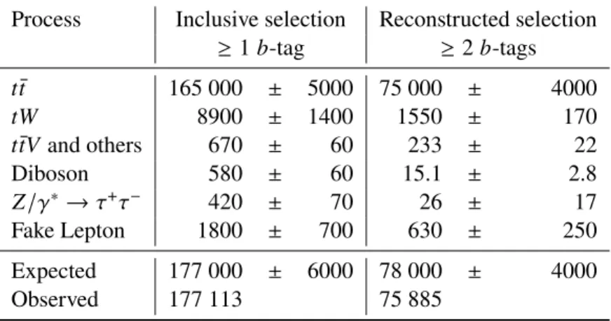
This is higher than the inclusive selection because of the tighter 𝑏-tagging requirement and because the 𝑡 ¯𝑡 reconstruction procedure tends to succeed more often for 𝑡 ¯𝑡 events than for background processes. The event yields after both selections are listed in Table1. The expected yields are in agreement with the observed number of events in both cases. Distributions of the lepton and jet 𝑝Tand 𝐸_Tmissare shown in

Figure1for the inclusive selection. The data and prediction agree within the total uncertainty for all of these kinematic observables. The trends observed in the lepton and jet 𝑝Tarise from the well-documented

limitations of the modelling of the top quark’s 𝑝Tspectrum at NLO [64–66]. The systematic uncertainties

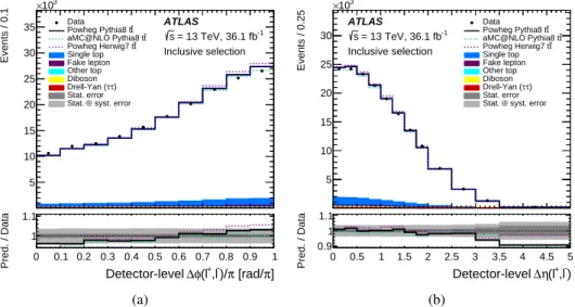
included in both the table and the figures are described in Section6. The azimuthal opening angle of the electron and muon, Δ𝜙, and the absolute value of the separation of the leptons in pseudorapidity, Δ𝜂, are shown in Figure2for the inclusive selection. The observed distribution is compared to the sum of signal and background using three different signal models: Powheg +Pythia 8, Powheg +Herwig 7, and MadGraph5_aMC@NLO +Pythia 8, and the ratio panel compares the combined signal plus background to data for the three models.

Table 1: Event yields in the inclusive and reconstructed selections for the observed data, expected signal and expected background. The uncertainties quoted include contributions from leptons, jets, missing transverse momentum, luminosity, background modelling, and pile-up modelling. They do not include uncertainties from PDF or signal 𝑡 ¯𝑡 modelling. The “𝑡 ¯𝑡𝑉 and others” entries contain events from 𝑡 ¯𝑡𝑍 , 𝑡 ¯𝑡𝑊 , 𝑡 ¯𝑡𝑊𝑊 , 𝑡 ¯𝑡𝐻, and the 𝑡 ¯𝑡𝑡 ¯𝑡 processes.

Process Inclusive selection Reconstructed selection

≥ 1 𝑏-tag ≥ 2 𝑏-tags 𝑡_¯𝑡 _{165 000} ± ₅₀₀₀ _{75 000} ± ₄₀₀₀ 𝑡𝑊 ₈₉₀₀ ± ₁₄₀₀ ₁₅₅₀ ± ₁₇₀ 𝑡_{¯𝑡𝑉 and others} ₆₇₀ ± ₆₀ ₂₃₃ ± ₂₂ Diboson 580 ± 60 15.1 ± 2.8 𝑍/𝛾∗→ 𝜏+𝜏− ₄₂₀ ± ₇₀ ₂₆ ± ₁₇ Fake Lepton 1800 ± 700 630 ± 250 Expected 177 000 ± 6000 78 000 ± 4000 Observed 177 113 75 885

4.2 Reconstruction of the 𝒕 ¯𝒕 system

In order to measure spin correlations as a function of the 𝑡 ¯𝑡 invariant mass at detector level, the kinematic properties of the event must be reconstructed from the identified leptons, jets, and missing transverse momentum. The top quark, top antiquark, and reconstructed 𝑡 ¯𝑡 system are built using the Neutrino Weighting (NW) method [67]. While the individual four-momenta of the two neutrinos in the final state are not directly measured in the detector, the sum of their transverse momenta is measured as 𝐸_Tmiss. The absence of the measured four-momenta of the two neutrinos leads to an under-constrained system that cannot be solved analytically. The following invariant mass constraints were applied to each event:

(ℓ_1,2+ 𝜈_1,2)2_{= 𝑚}2 𝑊 = (80.4 GeV) 2_, (ℓ_1,2+ 𝜈_1,2+ 𝑏_1,2)2_{= 𝑚}2 𝑡 = (172.5 GeV) 2 , (1)

(10)

(e) [GeV] T Detector-level p 50 100 150 200 250 Events / GeV 10 2 10 3 10 4 10 5 10 Data t Powheg Pythia8 t t aMC@NLO Pythia8 t t Powheg Herwig7 t Single top Fake lepton Other top Diboson ) τ τ Drell-Yan ( Stat. error syst. error ⊕ Stat. Inclusive selection ATLAS -1 = 13 TeV, 36.1 fb s (e) [GeV] T Detector-level p 50 100 150 200 250 Pred. / Data 0.9 1 1.1 (a) ) [GeV] µ ( T Detector-level p 50 100 150 200 250 Events / GeV 10 2 10 3 10 4 10 5 10 Data t Powheg Pythia8 t t aMC@NLO Pythia8 t t Powheg Herwig7 t Single top Fake lepton Other top Diboson ) τ τ Drell-Yan ( Stat. error syst. error ⊕ Stat. Inclusive selection ATLAS -1 = 13 TeV, 36.1 fb s ) [GeV] µ ( T Detector-level p 50 100 150 200 250 Pred. / Data 0.9 1 1.1 (b) (b-jet) [GeV] T Detector-level p 50 100 150 200 250 Events / GeV 2 10 3 10 4 10 5

10 Data_{Powheg Pythia8 t}_t

t aMC@NLO Pythia8 t t Powheg Herwig7 t Single top Fake lepton Other top Diboson ) τ τ Drell-Yan ( Stat. error syst. error ⊕ Stat. Inclusive selection ATLAS -1 = 13 TeV, 36.1 fb s (b-jet) [GeV] T Detector-level p 50 100 150 200 250 Pred. / Data 0.9 1 1.1 (c) [GeV] miss T Detector-level E 0 50 100 150 200 250 Events / GeV 10 2 10 3 10 4 10 Data t Powheg Pythia8 t t aMC@NLO Pythia8 t t Powheg Herwig7 t Single top Fake lepton Other top Diboson ) τ τ Drell-Yan ( Stat. error syst. error ⊕ Stat. Inclusive selection ATLAS -1 = 13 TeV, 36.1 fb s [GeV] miss T Detector-level E 0 50 100 150 200 250 Pred. / Data 0.9 1 1.1 (d)

Figure 1: Kinematic distributions for the (a) electron 𝑝T, (b) muon 𝑝T, (c) leading 𝑏-jet 𝑝T, and (d) 𝐸_Tmissfor the 𝑒 ±

𝜇∓ inclusive selection. In all figures, the rightmost bin also contains events that are above the 𝑥-axis range. The dark uncertainty bands in the ratio plots represent the statistical uncertainties while the light uncertainty bands represent the statistical and systematic uncertainties added in quadrature. The systematic uncertainties include contributions from leptons, jets, missing transverse momentum, background modelling, pile-up modelling and luminosity, but not PDF or signal 𝑡 ¯𝑡 modelling uncertainties. The observed distribution is compared to the sum of signal and background using three different 𝑡 ¯𝑡 signal models: Powheg +Pythia 8, Powheg +Herwig 7 and MadGraph5_aMC@NLO +Pythia 8, and the ratio panel compares the summed prediction to data for the three models.

(11)

] π [rad/ π )/ -,l + (l φ ∆ Detector-level 0 0.1 0.2 0.3 0.4 0.5 0.6 0.7 0.8 0.9 1 Events / 0.1 5 10 15 20 25 30 35 3 10 × Data t Powheg Pythia8 t t aMC@NLO Pythia8 t t Powheg Herwig7 t Single top Fake lepton Other top Diboson ) τ τ Drell-Yan ( Stat. error syst. error ⊕ Stat. Inclusive selection ATLAS -1 = 13 TeV, 36.1 fb s ] π [rad/ π )/ -,l + (l φ ∆ Detector-level 0 0.1 0.2 0.3 0.4 0.5 0.6 0.7 0.8 0.9 1 Pred. / Data 1 1.1 (a) ) -,l + (l η ∆ Detector-level 0 0.5 1 1.5 2 2.5 3 3.5 4 4.5 5 Events / 0.25 5 10 15 20 25 30 3 10 × Data t Powheg Pythia8 t t aMC@NLO Pythia8 t t Powheg Herwig7 t Single top Fake lepton Other top Diboson ) τ τ Drell-Yan ( Stat. error syst. error ⊕ Stat. ATLAS -1 = 13 TeV, 36.1 fb s Inclusive selection ) -,l + (l η ∆ Detector-level 0 0.5 1 1.5 2 2.5 3 3.5 4 4.5 5 Pred. / Data 0.9 1 1.1 (b)

Figure 2: Distribution of (a) the Δ𝜙 and (b) Δ𝜂 observables for the 𝑒 𝜇 selection after the requirement of at least one 𝑏_{-tagged jet (inclusive selection). The highest bin for Δ𝜂 also contains events that are above the 𝑥-axis range. The dark} uncertainty bands in the ratio plots represent the statistical uncertainties while the light uncertainty bands represent the statistical and systematic uncertainties added in quadrature. The systematic uncertainties include contributions from leptons, jets, missing transverse momentum, background modelling, pile-up modelling and luminosity, but not PDF or signal 𝑡 ¯𝑡 modelling uncertainties. The observed distribution is compared to the sum of signal and background using three different 𝑡 ¯𝑡 signal models: Powheg +Pythia 8, Powheg +Herwig 7 and MadGraph5_aMC@NLO +Pythia 8, and the ratio panel compares the summed prediction to data for the three models.

where ℓ1,2, 𝜈1,2 and 𝑏1,2 represent the four-momenta of the charged leptons, neutrinos and 𝑏-quarks,

respectively. Since the neutrino pseudorapidities (𝜂(𝜈) and 𝜂( ¯𝜈_{)) required for 𝜈}

1,2 are unknown, their

values are scanned, in steps of 0.2, between −5 and 5.

With the assumptions about 𝑚𝑡, 𝑚𝑊 and values for 𝜂(𝜈) and 𝜂( ¯𝜈), Eq. (1) can now be solved, leading to

two possible solutions for each assumption of 𝜂(𝜈) and 𝜂( ¯𝜈). Only real solutions without an imaginary component are considered. An “inferred” 𝐸_Tmissvalue, resulting from the neutrinos for each solution, is compared to the 𝐸_Tmissobserved in the event. A weight is introduced in order to quantify this agreement:

𝑤= exp −Δ𝐸2 𝑥 2𝜎𝑥2 ! · exp −Δ𝐸 2 𝑦 2𝜎𝑦2 ! ,

where Δ𝐸𝑥 , 𝑦 is the difference between the (𝑥,𝑦) component of the missing transverse momentum computed

from the neutrino four momenta in Eq. (1) and the observed missing transverse momentum, and 𝜎𝑥 , 𝑦is a

fixed scale related to the resolution of the observed 𝐸_Tmissin the detector in (𝑥, 𝑦), based on studies in 𝑍 boson events [63]. The assumption for 𝜂(𝜈) and 𝜂( ¯𝜈) that gives the highest weight is used to reconstruct the 𝑡 and ¯𝑡 quarks for that event.

In each event, there may be more than two 𝑏-tagged jets (on average there are 2.04 𝑏-tagged jets per event) and therefore several possible combinations of jets to use in the kinematic reconstruction. In addition, there is an ambiguity in assigning a jet to the 𝑡 or ¯𝑡 quark candidate. To reduce this ambiguity, the two 𝑏_{-tagged jets with the highest weight from the 𝑏-tagging algorithm are used to reconstruct the 𝑡 and ¯𝑡} quarks and the assignment which produces the solution with highest weight in the NW is taken as the correct assignment.

(12)

Equation (1) cannot always be solved for a particular assumption of 𝜂(𝜈) and 𝜂( ¯𝜈). This can be caused by mis-assignment of the input objects or through mis-measurement of the input object four-momenta. It is also possible that the assumed 𝑚𝑡is sufficiently different from the true value to prevent a valid solution for

a particular event, or the event is from a background process, and therefore cannot be solved. To mitigate these effects, the assumed value of 𝑚𝑡 is scanned between the values of 171 and 174 GeV, in steps of 0.5

GeV, and the 𝑝T of the measured jets are smeared using a Gaussian function with a 𝑝T-dependent width

between 14% and 8% of their measured 𝑝T. This smearing is repeated 5 times.

This procedure allows the NW algorithm to shift the four-momenta of the two jets and the 𝑚𝑡 hypothesis

to see if a solution can be found. The solution which produces the highest 𝑤 gives the kinematics of the reconstructed event. Solutions which provide an invariant mass of the 𝑡 ¯𝑡 system below 300 GeV, or which provide 𝑡 or ¯𝑡 quarks with negative energies, are rejected. For around 5% of events, no solution can be found, even after smearing. Only events with at least one solution with a weight above 0.4 are considered, where this criterion was chosen to optimise the angular resolution in the top quark reconstruction. The efficiency for 𝑡_{¯𝑡 reconstruction is}∼_{80%. Due to the implicit assumptions about 𝑚}𝑡and 𝑚𝑊, the reconstruction efficiency

found in simulated background samples is much lower (∼_{60% for 𝑡𝑊 and Drell–Yan processes) and leads to}

a suppression of background events. Table1shows the event yields before and after reconstruction in the signal region. The different effects of the systematic uncertainties on each type of selection are discussed in greater detail in Section7.

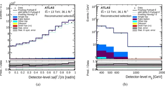
Figure3shows the distributions of Δ𝜙 and 𝑚𝑡𝑡_¯after reconstruction and with a requirement of at least two

𝑏_{-tagged jets (reconstructed selection). The four plots in Figure}₄_{show the Δ𝜙 distribution split into four} mass regions: 𝑚𝑡_¯𝑡 <450 GeV; 450 ≤ 𝑚𝑡𝑡_¯< 550 GeV; 550 ≤ 𝑚𝑡𝑡_¯ <800 GeV; and 𝑚𝑡𝑡_¯ ≥ 800 GeV. These

bins in 𝑚𝑡𝑡_¯were determined to have the finest possible granularity whilst maintaining an unbiased and

stable unfolding procedure for the Δ𝜙 observable (described further in Section5).

4.3 Definitions of partons and particles

In the measurements presented in this paper, events are corrected for detector effects using two definitions of particles in the generator-level record of the simulation: parton level and particle level. Parton-level objects are taken from the MC simulation history. Top quarks are taken after radiation but before decay (this is the last top quark in a decay chain) whereas leptons are taken before radiation (i.e. Born level leptons). The measurement corrected to parton level is extrapolated to the full phase-space, where all generated dilepton events are considered. However, events with leptons originating from an intermediate 𝜏_{-lepton in the 𝑡 → 𝑏𝑊 → 𝑏ℓ𝜈 decay chain are not considered as their subsequent decays do not carry the} full spin information of their parent top quark and hence, dilute the spin correlation information. Fiducial requirements are not made on the partonic objects so that the results at parton level can be more easily compared to fixed-order predictions.

Particle-level objects are constructed using a procedure intended to correspond as closely as possible to the detector-level object and event selection. Only objects in the MC simulation considered stable (with lifetimes longer than 3 × 10−11s) in the generator-level information are used. Particle-level leptons are identified as those originating from a 𝑊 boson decay. The four-momentum of each electron or muon is summed with the four-momenta of all radiated photons within a cone of size Δ𝑅 = 0.1 about its direction, excluding photons from hadron decays. The resulting leptons are required to have 𝑝T > 25 GeV

and |𝜂| < 2.5. Particle-level jets are constructed using stable particles, with the exception of selected particle-level electrons and muons, photons that are summed into the electrons or muons, and particle-level

(13)

] π [rad/ π )/ -,l + (l φ ∆ Detector-level 0 0.1 0.2 0.3 0.4 0.5 0.6 0.7 0.8 0.9 1 Events / 0.1 2 4 6 8 10 12 14 16 3 10 × Data t Powheg Pythia8 t t aMC@NLO Pythia8 t t Powheg Herwig7 t Single top Fake lepton Other top Diboson ) τ τ Drell-Yan ( Stat. error syst. error ⊕ Stat. Reconstructed selection ATLAS -1 = 13 TeV, 36.1 fb s ] π [rad/ π )/ -,l + (l φ ∆ Detector-level 0 0.1 0.2 0.3 0.4 0.5 0.6 0.7 0.8 0.9 1 Pred. / Data 0.9 1 1.1 (a) [GeV] t t Detector-level m 3 10 Events / GeV 1 10 2 10 3 10 4 10 Data t Powheg Pythia8 t t aMC@NLO Pythia8 t t Powheg Herwig7 t Single top Fake lepton Other top Diboson ) τ τ Drell-Yan ( Stat. error syst. error ⊕ Stat. ATLAS -1 = 13 TeV, 36.1 fb s Reconstructed selection [GeV] t t Detector-level m 400 500 600 1000 2000 Pred. / Data 0.9 1 1.1 (b)

Figure 3: Kinematic distributions for (a) Δ𝜙 and (b) 𝑚𝑡_¯𝑡after the requirement of at least two 𝑏-tagged jets and Neutrino Weighting (reconstructed selection). The highest bin in Figure3(b)also contains events that are above the 𝑥-axis range. The dark uncertainty bands in the ratio plots represent the statistical uncertainties while the light uncertainty bands represent the statistical and systematic uncertainties added in quadrature. The systematic uncertainties include contributions from leptons, jets, missing transverse momentum, background modelling, pile-up modelling and luminosity, but not PDF or signal 𝑡 ¯𝑡 modelling uncertainties. The observed distribution is compared to the sum of signal and background using three different 𝑡 ¯𝑡 signal models: Powheg +Pythia 8, Powheg +Herwig 7, and MadGraph5_aMC@NLO +Pythia 8, and the ratio panel compares the summed prediction to data for the three models.

neutrinos originating from 𝑊 boson decays. The jets are constructed using the anti-𝑘𝑡 algorithm with a

radius parameter of 𝑅 = 0.4, and selected if they pass the requirements of 𝑝T > 25 GeV and |𝜂| < 2.5.

Intermediate 𝑏-hadrons in the MC decay chain history are clustered in the stable-particle jets with their energies set to zero. If, after clustering, a particle-level jet contains one or more of these “ghost” 𝑏-hadrons, the jet is said to have originated from a 𝑏-quark. This technique is referred to as “ghost matching” [59]. Particle-level 𝐸_Tmissis calculated using the vector transverse-momentum sum of all neutrinos in the event, excluding those originating from hadron decays, either directly or via a 𝜏-lepton.

Events are selected at the particle level in a fiducial phase-space region with similar requirements to the phase-space region in the detector. They must contain exactly one particle-level electron and one particle-level muon of opposite electric charge, at least one of which must have 𝑝T >27 GeV, and at least

two particle-level jets. The particle-level requirement on the number of jets that must be ghost-matched to a 𝑏-hadron mimics the inclusive and reconstructed selections at detector-level: for the inclusive selection, at least one particle-level jet must be ghost-matched, while for the reconstructed case, the particle-level selection requires exactly two ghost-matched jets. In addition, the reconstructed selection excludes particle-level leptons originating from an intermediate 𝜏-lepton in the 𝑡 → 𝑏𝑊 → 𝑏ℓ𝜈 decay chain. The particle-level 𝑡 ¯𝑡 object is constructed using the sum of the particle-level electron and muon, the two ghost-matched jets, and the two neutrinos that originate from the same 𝑊 boson decays as the selected particle-level leptons.

(14)

] π [rad/ π )/ -,l + (l φ ∆ Detector-level 0 0.1 0.2 0.3 0.4 0.5 0.6 0.7 0.8 0.9 1 Events / 0.1 1000 2000 3000 4000 5000 6000 Data t Powheg Pythia8 t t aMC@NLO Pythia8 t t Powheg Herwig7 t Single top Fake lepton Other top Diboson ) τ τ Drell-Yan ( Stat. error syst. error ⊕ Stat. < 450 GeV t t m Reconstructed selection ATLAS -1 = 13 TeV, 36.1 fb s ] π [rad/ π )/ -,l + (l φ ∆ Detector-level 0 0.1 0.2 0.3 0.4 0.5 0.6 0.7 0.8 0.9 1 Pred. / Data 0.9 1 1.1 (a) ] π [rad/ π )/ -,l + (l φ ∆ Detector-level 0 0.1 0.2 0.3 0.4 0.5 0.6 0.7 0.8 0.9 1 Events / 0.1 1000 2000 3000 4000 5000

6000 DataPowheg Pythia8 tt t aMC@NLO Pythia8 t t Powheg Herwig7 t Single top Fake lepton Other top Diboson ) τ τ Drell-Yan ( Stat. error syst. error ⊕ Stat. < 550 GeV t t m ≤ 450 Reconstructed selection ATLAS -1 = 13 TeV, 36.1 fb s ] π [rad/ π )/ -,l + (l φ ∆ Detector-level 0 0.1 0.2 0.3 0.4 0.5 0.6 0.7 0.8 0.9 1 Pred. / Data 0.9 1 1.1 (b) ] π [rad/ π )/ -,l + (l φ ∆ Detector-level 0 0.1 0.2 0.3 0.4 0.5 0.6 0.7 0.8 0.9 1 Events / 0.1 1000 2000 3000 4000 5000 6000 7000

8000 DataPowheg Pythia8 tt t aMC@NLO Pythia8 t t Powheg Herwig7 t Single top Fake lepton Other top Diboson ) τ τ Drell-Yan ( Stat. error syst. error ⊕ Stat. < 800 GeV t t m ≤ 550 Reconstructed selection ATLAS -1 = 13 TeV, 36.1 fb s ] π [rad/ π )/ -,l + (l φ ∆ Detector-level 0 0.1 0.2 0.3 0.4 0.5 0.6 0.7 0.8 0.9 1 Pred. / Data 0.9 1 1.1 (c) ] π [rad/ π )/ -,l + (l φ ∆ Detector-level 0 0.1 0.2 0.3 0.4 0.5 0.6 0.7 0.8 0.9 1 Events / 0.1 500 1000 1500 2000 2500 3000 3500 4000 4500 _Data t Powheg Pythia8 t t aMC@NLO Pythia8 t t Powheg Herwig7 t Single top Fake lepton Other top Diboson ) τ τ Drell-Yan ( Stat. error syst. error ⊕ Stat. 800 GeV ≥ t t m Reconstructed selection ATLAS -1 = 13 TeV, 36.1 fb s ] π [rad/ π )/ -,l + (l φ ∆ Detector-level 0 0.1 0.2 0.3 0.4 0.5 0.6 0.7 0.8 0.9 1 Pred. / Data 0.9 1 1.1 (d)

Figure 4: Kinematic distributions after the requirement of at least two 𝑏-tagged jets and Neutrino Weighting (reconstructed selection). The plots display Δ𝜙/𝜋 in individual mass ranges: (a) 𝑚𝑡𝑡_¯ < 450 GeV, (b) 450 ≤ 𝑚_𝑡

¯

𝑡 < 550 GeV, (c) 550 ≤ 𝑚𝑡𝑡_¯ < 800 GeV, and (d) 𝑚𝑡𝑡_¯ ≥ 800 GeV. The dark uncertainty bands in the ratio plots represent the statistical uncertainties while the light uncertainty bands represent the statistical and systematic uncertainties added in quadrature. The systematic uncertainties include contributions from leptons, jets, missing transverse momentum, background modelling, pile-up modelling and luminosity, but not PDF or signal 𝑡 ¯𝑡 modelling uncertainties. The observed distribution is compared to the sum of signal and background using three different 𝑡 ¯𝑡 signal models: Powheg +Pythia 8, Powheg +Herwig 7 and MadGraph5_aMC@NLO +Pythia 8, and the ratio panel compares the summed prediction to data for the three models.

(15)

5 Unfolding procedure

The data are corrected for detector resolution and acceptance effects using an iterative Bayesian unfolding procedure [68] in order to create distributions at particle (parton) level in a fiducial (full) phase-space. The unfolding itself is performed using the RooUnfold package [69].

In the unfolding procedure, background-subtracted data are corrected for detector acceptance and resolution effects as well as for the efficiency to pass the event selection requirements in order to obtain the absolute differential cross-sections: d𝜎𝑡𝑡_¯ d𝑋𝑖 = 1 L · Δ𝑋𝑖 · 𝜖𝑖 eff ·∑︁ 𝑗 𝑅−1 𝑖 𝑗 · 𝑓 𝑗 acc· (𝑁 𝑗 obs− 𝑁 𝑗 bkg),

where 𝑗 is the index for bins of observable 𝑋 at detector level and 𝑖 labels the bins at particle or parton level. Δ𝑋𝑖is the width of bin 𝑖, 𝑁

𝑗

obsis the number of observed events in data in bin 𝑗 , L is the integrated

luminosity, 𝑁

𝑗

bkg is the estimated number of background events in bin 𝑗 , 𝑅 is the response matrix and

𝑅−1

𝑖 𝑗 symbolises the effective inversion of 𝑅 in the Bayesian unfolding. The acceptance correction 𝑓 𝑗 acc

accounts for events that are outside the fiducial phase-space but pass the detector-level selection. The efficiency correction 𝜖_eff𝑖 corrects for events that are in the fiducial phase-space but are not reconstructed in the detector.

The fiducial differential cross-sections are divided by the measured total cross-section, obtained by integrating over all bins in the differential distribution, in order to obtain the normalised differential cross-sections. The response matrix, 𝑅, describes the detector response and is determined by mapping the bin-to-bin migration of events from particle or parton level to detector level in the nominal 𝑡 ¯𝑡 MC simulation. Figure5(a)and5(b)illustrate the response matrices that are used for the single-differential Δ𝜙 and Δ𝜂 observables at parton level. Each response matrix is normalised such that the sum of entries in each row is equal to one. The values represent the fraction of events at either particle or parton level in bin 𝑖 that are reconstructed in bin 𝑗 at detector level. Figure5(c)shows the response matrix for the double-differential distribution of Δ𝜙 as a function of 𝑚𝑡𝑡_¯at parton level. The Δ𝜙 distributions for each 𝑚𝑡𝑡_¯

region are concatenated into a single one-dimensional distribution, such that the response matrix takes into account the migrations between different 𝑚𝑡𝑡_¯regions. As can be observed in the figure, the Δ𝜙 observable

is diagonal in each region, with the majority of the off-diagonal smearing occurring due to the resolution of the 𝑚𝑡𝑡_¯observable.

The binning for each observable is chosen in order to minimise the effect of statistical fluctuations in the data as well as in the alternative 𝑡 ¯𝑡 samples which are used in the systematic prescription (and are a dominant source of systematic uncertainty), as well as to account for the experimental resolution. The size of the chosen bins is usually much larger than the detector resolution on the Δ𝜙 observable, which is illustrated by the highly diagonal response matrices in the inclusive selection. In contrast, the resolution of the reconstructed 𝑚𝑡𝑡_¯observable is significantly larger and so the binning here is chosen to be the smallest

possible binning that reproduces the underlying truth-level distribution without bias, when measured using MC pseudo-experiments.

The stability of the unfolding procedure is determined by constructing pseudo-data sets by randomly sampling events from the nominal 𝑡 ¯𝑡 MC sample with approximately the same statistical power as the expected data. Pull tests are performed as part of the binning optimisation and are therefore always successful for the chosen observable bins. In addition, the unfolding procedure is tested to see how

(16)

it responds to various stresses introduced into the pseudo-data. Three such stresses are investigated: introducing linear slopes in the observables, the difference between the spin correlated and uncorrelated MC samples, and the observed difference between data and the expectation at detector level. In all cases, the unfolding procedure is able to correct the pseudo-data back to their underlying truth spectra and so a systematic uncertainty for the unfolding procedure is not included.

The number of iterations used in the iterative Bayesian unfolding is also optimised using pseudo-experiments. Iterations are performed until the 𝜒2per degree-of-freedom, calculated by comparing the unfolded pseudo-data to the corresponding generator-level distribution for that pseudo-pseudo-data set, is less than or equal to unity. For the inclusive observables (Δ𝜙 and Δ𝜂), the optimal number of iterations is determined to be two, whereas for the reconstructed observable (Δ𝜙 in bins of 𝑚𝑡𝑡_¯), the optimal number of iterations is

(17)

Migration [%] 0 10 20 30 40 50 60 70 80 90 100 99.5 99.2 99.2 99.2 99.2 99.2 99.3 99.3 99.4 99.6 ] π [rad/ π )/ -,l + (l φ ∆ Detector-level 0.1 − 0.0 0.2 − 0.1 0.3 − 0.2 0.4 − 0.3 0.5 − 0.4 0.6 − 0.5 0.7 − 0.6 0.8 − 0.7 0.9 − 0.8 1.0 − 0.9 ] π [rad/ π )/ -,l + (l φ∆ Parton-level 0.1 − 0.0 0.2− 0.1 0.3− 0.2 0.4− 0.3 0.5 − 0.4 0.6− 0.5 0.7 − 0.6 0.8− 0.7 0.9− 0.8 1.0− 0.9 0.4 0.4 0.4 0.3 0.4 0.3 0.4 0.3 0.4 0.3 0.4 0.3 0.4 0.3 0.4 0.3 0.3 0.3 0 10 20 30 40 50 60 70 80 90 100

ATLAS Simulation _s_{= 13 TeV, 36.1 fb}-1

(a) Migration [%] 0 10 20 30 40 50 60 70 80 90 100 99.5 99.1 99.1 99.1 99.1 99.1 99.1 99.2 99.5 99.5 99.5 99.5 ) -,l + (l η ∆ Detector-level 0.3 − 0.0 0.5 − 0.3 0.8 − 0.5 1.0 − 0.8 1.3 − 1.0 1.5 − 1.3 1.8 − 1.5 2.0 − 1.8 2.5 − 2.0 3.0 − 2.5 3.5 − 3.0 5.0 − 3.5 ) - _,l + (l η∆ Parton-level 0.3− 0.0 0.5− 0.3 0.8− 0.5 1.0− 0.8 1.3− 1.0 1.5 − 1.3 1.8 − 1.5 2.0− 1.8 2.5− 2.0 3.0− 2.5 3.5− 3.0 5.0− 3.5 0.4 0.5 0.4 0.4 0.4 0.5 0.4 0.5 0.4 0.4 0.4 0.5 0.4 0.4 0.4 0.3 0.2 0.4 0.1 0.4 0.1 0.1 0.4 0 10 20 30 40 50 60 70 80 90 100

ATLAS Simulation _s_{= 13 TeV, 36.1 fb}-1

(b) Migration [%] 0 10 20 30 40 50 60 70 80 90 100 82 78 70 64 60 43 45 45 46 56 58 60 61 72 79 ] π [rad/ π )/ -,l + (l φ ∆ Detector-level < 450 GeV tt m < 550 GeV t t m ≤ 450 < 800 GeV t t m ≤ 550 800 GeV ≥ tt m ] π [rad/ π )/ - _,l + (l φ∆ Parton-level 0.2 − 0.0 0.4 − 0.2 0.6 − 0.4 0.8 − 0.6 1.0 − 0.8 0.3 − 0.0 0.6 − 0.3 0.8 − 0.6 1.0 − 0.8 0.4 − 0.0 0.6 − 0.4 0.8 − 0.6 1.0 − 0.8 0.8 − 0.0 1.0 − 0.8 14 3 8 9 4 22 7 1 25 9 1 26 11 2 24 14 17 1 10 21 5 17 2 24 26 4 22 27 4 5 7 15 7 10 9 21 13 6 17 17 5 15 19 1 1 1 5 6 14 1 1 19 0 10 20 30 40 50 60 70 80 90 100

ATLAS Simulation s = 13 TeV, 36.1 fb-1

(c)

Figure 5: Parton-level response matrices, normalised by row and shown as percentages, for: (a) Δ𝜙, (b) Δ𝜂, and (c) Δ𝜙 as a function of 𝑚𝑡𝑡_¯, after Neutrino Weighting. For (c), the binning on the horizontal and vertical axes is identical, with each invariant mass region subdivided into Δ𝜙 bins. The dotted lines separate different invariant mass regions, while the tick marks indicate the Δ𝜙 bins.

(18)

6 Systematic uncertainties

The measured differential cross-sections are affected by systematic uncertainties arising from detector response, signal modelling, and background modelling. The contributions from various sources of uncertainty are described in this section. These individual systematic uncertainties are summed in quadrature to obtain the total systematic uncertainty, and the overall uncertainty is calculated by summing the systematic and statistical uncertainties in quadrature.

6.1 Signal modelling uncertainties

The following four systematic uncertainties related to the modelling of the 𝑡 ¯𝑡 system in the MC generators are considered: the choice of matrix-element generator, the hadronisation and parton-shower model, the amount of initial- and final-state radiation, and the choice of PDF set. In each case (except for the PDF uncertainty), alternative MC samples are unfolded with the nominal 𝑡 ¯𝑡 MC response and the difference to their generator-level spectra is taken as the systematic uncertainty. A fast detector simulation (described in Section3) is used for each of the alternative models and for the response matrix, rather than the full detector simulation used in the nominal unfolding procedure. In most cases, the resulting systematic shift is used to define a symmetric uncertainty, where deviations from the generator-level spectra are also considered to be mirrored in the opposite direction, resulting in equal and opposite symmetric uncertainties (called symmetrising).

The choice of NLO ME generator affects the invariant mass of the simulated 𝑡 ¯𝑡 events, the observables them-selves, and the reconstruction efficiencies. To estimate this uncertainty, MadGraph5_aMC@NLO (with Pythia8 for the parton-shower simulation) is used, applying the nominal unfolding procedure based on the Powheg-Box+Pythia 8 𝑡 ¯𝑡 sample. The resulting uncertainty is symmetrised.

To evaluate the uncertainty arising from the choice of parton-shower algorithm and the hadronisation model, the alternative sample generated with Powheg-Box + Herwig 7 is unfolded with the nominal 𝑡 ¯𝑡 MC response. The resulting uncertainty is symmetrised.

The uncertainty arising from initial- and final-state radiation is evaluated using the reduced radiation sample of Powheg-Box + Pythia 8, and is again symmetrised. An enhanced radiation sample was also investigated as this has been used in previous similar analyses. However, it was found to markedly disagree with the data and is therefore not used here.

The uncertainty due to the choice of PDF set is evaluated using the PDF4LHC15 prescription [70], utilising 30 eigenvector shifts derived from fits to multiple NLO PDF sets. Each shift is evaluated for each bin added in quadrature and the resulting uncertainty in each bin is symmetrised.

6.2 Background modelling uncertainties

The uncertainties in the background processes are assessed by repeating the full analysis using pseudo-data sets and by varying the background predictions by one standard deviation of their nominal values. The difference between the nominal pseudo-data set result and the shifted result is taken as the systematic uncertainty, then the separate background uncertainties are combined in quadrature.

(19)

Each background prediction has an uncertainty associated with its theoretical section. The cross-section for the 𝑡𝑊 process is varied by ±5.3% [42], the diboson cross-section is varied by ±6%, and the Drell–Yan 𝑍 /𝛾∗→ 𝜏+𝜏−_{background cross-section is varied by ±5% based on studies of different MC} generators. Uncertainties on the remaining SM backgrounds are taken to be 13% for 𝑡 ¯𝑡𝑉 [36,71],+6.8_−9.9% for 𝑡 ¯𝑡𝐻 [72],+10₋₂₈% for 𝑡𝑊 𝑍 and ±50% for 𝑡 𝑍 , 𝑡 ¯𝑡𝑊𝑊 and 𝑡 ¯𝑡𝑡 ¯𝑡 [73].

An additional scaling factor and uncertainty of 1.07 ± 0.12 is assigned to the 𝑍 /𝛾∗background, based on a comparison of data and MC simulation in a region enriched in 𝑍 → ℓ+ℓ−_{decays in association with} 𝑏_-jets.

A 40% uncertainty is assigned to the normalisation of the fake-lepton background based on comparisons between data and MC simulation in a fake-dominated control region, which is selected in the same way as the 𝑡 ¯𝑡 signal region but the leptons are required to have same-sign electric charges. An additional uncertainty is included, to account for slight differences in shapes between the data-driven and MC estimates in Δ𝜙(ℓ+, ℓ−) and Δ𝜂(ℓ+, ℓ−).

An additional uncertainty is evaluated for the 𝑡𝑊 process by replacing the nominal DR sample with a DS sample, as discussed in Section3, and taking the difference between the two as the systematic uncertainty. Other background process uncertainties are found to be insignificant and are not discussed further.

6.3 Detector modelling uncertainties

Systematic uncertainties due to the modelling of the detector response affect the signal reconstruction efficiency, the unfolding procedure, and the background estimation. In order to evaluate their impact, the full analysis is repeated with variations of the detector modelling and the difference between the nominal and the shifted results is taken as the systematic uncertainty.

The uncertainties due to lepton isolation, trigger, identification, and reconstruction requirements are evaluated in data using a tag-and-probe method in events with a leptonically decaying 𝑍 boson [61,62]. The jet energy scale uncertainty is assessed in data [57], using simulation-based corrections and in situ techniques based on jets, photons and 𝑍 bosons. A 21-component breakdown of the uncertainty is used, with contributions from pile-up, jet flavour composition, single-particle response, and punch-through. The jet energy resolution uncertainty is parametrised as a function of jet 𝑝Tand rapidity [74].

Uncertainties related to the 𝑏-jet tagging procedure, summarised under “𝑏-tagging,” are determined separately for 𝑏-jets, 𝑐-jets and light-jets using a 27-component breakdown (6 for 𝑏-jets, 3 for 𝑐-jets, 16 for light-jets, and two extrapolation uncertainties) [60,75,76]. These uncertainties account for differences between data and simulation.

The systematic uncertainty due to the track-based terms (i.e. those tracks not associated with other reconstructed objects such as leptons and jets) used in the calculation of 𝐸miss_T is evaluated by comparing the 𝐸_Tmissin 𝑍 → 𝜇𝜇 events, which do not contain prompt neutrinos from the hard process, using different generators. Uncertainties associated with energy scales and resolutions of leptons and jets are propagated to the 𝐸miss_T calculation [63].

The uncertainty in the combined 2015+2016 integrated luminosity is 2.1%. It is derived, following a methodology similar to that detailed in Ref. [77], and using the LUCID-2 detector for the baseline luminosity measurements [78], from calibration of the luminosity scale using 𝑥 − 𝑦 beam–separation scans.

(20)

The uncertainty in the reweighting of the MC pile-up distribution to match the data is evaluated according to the uncertainty on the average number of interactions per bunch crossing.

7 Differential cross-section results

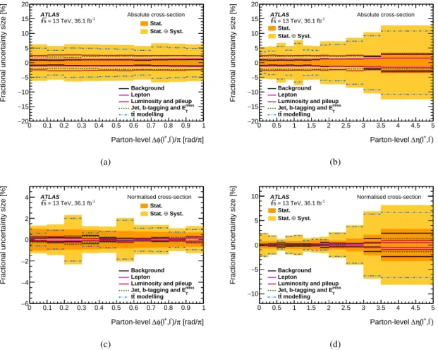
The absolute and normalised parton-level cross-sections for Δ𝜙 and Δ𝜂 are presented in Table2and Table3. These results are compared to several NLO MC generators interfaced to parton showers (described in Section3) in Figure6and the breakdown of the contributions to the systematic uncertainties are shown in Figure7. In each case, the total generator cross-section was normalised to the NNLO values described in Section3.

All uncertainties that are normalisation effects but which do not cause large changes in the shape of the observable (luminosity, for example) cancel when performing the normalised cross-sections. Jet and pile-up effects are also significant, but only in the absolute cross-sections. Overall, reasonable agreement is observed in the inclusive cross-section between the data and MC predictions but significant shape effects are apparent, particularly in the normalised observables where the uncertainties are small. Ignoring the differences in the absolute fiducial cross-sections between different MC generators, the shapes predicted by different generators are fairly consistent, except perhaps at very high Δ𝜂. In the Δ𝜙 observable, an obvious trend is observed, with the data tending to be higher than the expectation at low Δ𝜙 and lower than the expectation at high Δ𝜙. For Δ𝜂, the data and expectation agree well at low values, even in the normalised cross-sections, but there is a slight tension at higher values.

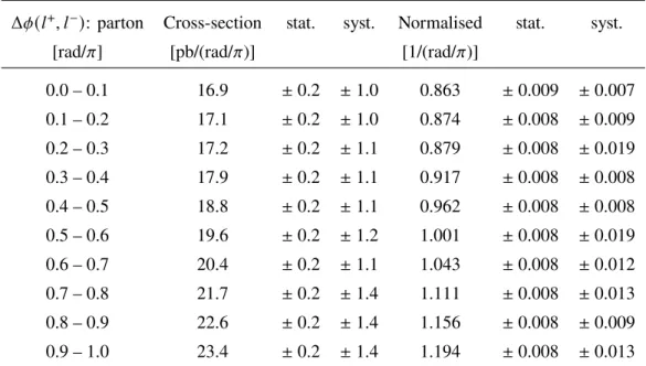
Table 2: Summary of the parton-level absolute and normalised differential cross-sections as a function of Δ𝜙(ℓ+, ℓ−), with statistical and systematic uncertainties in each bin.

Δ𝜙(𝑙+, 𝑙−): parton _{Cross-section} _stat. _syst. _Normalised _stat. _syst.

[rad/𝜋] [pb/(rad/𝜋)] [1/(rad/𝜋)]

0.0 – 0.1 16.9 ± 0.2 ± 1.0 0.863 ± 0.009 ± 0.007 0.1 – 0.2 17.1 ± 0.2 ± 1.0 0.874 ± 0.008 ± 0.009 0.2 – 0.3 17.2 ± 0.2 ± 1.1 0.879 ± 0.008 ± 0.019 0.3 – 0.4 17.9 ± 0.2 ± 1.1 0.917 ± 0.008 ± 0.008 0.4 – 0.5 18.8 ± 0.2 ± 1.1 0.962 ± 0.008 ± 0.008 0.5 – 0.6 19.6 ± 0.2 ± 1.2 1.001 ± 0.008 ± 0.019 0.6 – 0.7 20.4 ± 0.2 ± 1.1 1.043 ± 0.008 ± 0.012 0.7 – 0.8 21.7 ± 0.2 ± 1.4 1.111 ± 0.008 ± 0.013 0.8 – 0.9 22.6 ± 0.2 ± 1.4 1.156 ± 0.008 ± 0.009 0.9 – 1.0 23.4 ± 0.2 ± 1.4 1.194 ± 0.008 ± 0.013

The unfolded, normalised parton-level cross-sections for Δ𝜙 in four 𝑡 ¯𝑡 invariant mass bins are shown in Table4. They are compared with different NLO ME generators and parton showers in Figure8and the systematic uncertainties are illustrated in Figure9. Each differential cross-section is normalised within its

(21)

10.0 12.5 15.0 17.5 20.0 22.5 25.0 d σ d ∆φ (l +,l −)/ π [pb/(r ad/ π )] √_{s = 13 TeV, 36.1 fb}₋₁ ATLAS Data Powheg Pythia8 Powheg Herwig7 MG5 aMC@NLO Pythia8 Sherpa Powheg Pythia6 PowPy8 rad. down

0.2 0.4 0.6 0.8 Parton-level ∆φ(l+_{, l}−_{)/π [rad/π]} 0.95 1.00 1.05 1.10 Theor y Data Stat. Total (a) 0.0 2.5 5.0 7.5 10.0 12.5 15.0 d σ d ∆η (l +,l −) [pb/(unit η )] √_{s = 13 TeV, 36.1 fb}₋₁ ATLAS Data Powheg Pythia8 Powheg Herwig7 MG5 aMC@NLO Pythia8 Sherpa Powheg Pythia6 PowPy8 rad. down

1 2 3 4 Parton-level ∆η(l+_{, l}−₎ 0.9 1.0 1.1 1.2 Theor y Data Stat. Total (b) 0.6 0.8 1.0 1.2 1 · σ d σ d ∆φ (l +,l −)/ π [1/(r ad/ π )] √ s = 13 TeV, 36.1 fb−1 ATLAS Data Powheg Pythia8 Powheg Herwig7 MG5 aMC@NLO Pythia8 Sherpa Powheg Pythia6 PowPy8 rad. down

0.2 0.4 0.6 0.8 Parton-level ∆φ(l+_{, l}−_{)/π [rad/π]} 0.95 1.00 1.05 Theor y Data Stat. Total (c) 0.0 0.2 0.4 0.6 1 · σ d σ d ∆η (l +,l −) [1/(unit η )] √ s = 13 TeV, 36.1 fb−1 ATLAS Data Powheg Pythia8 Powheg Herwig7 MG5 aMC@NLO Pythia8 Sherpa Powheg Pythia6 PowPy8 rad. down

1 2 3 4 Parton-level ∆η(l+_{, l}−₎ 0.9 1.0 1.1 Theor y Data Stat. Total (d)

Figure 6: The parton-level differential cross-sections compared to predictions from Powheg, Mad-Graph5_aMC@NLO and Sherpa: (top), absolute (a) Δ𝜙 and (b) Δ𝜂 and (bottom), normalised (c) Δ𝜙 and (d) Δ𝜂, using the inclusive selection.

(22)

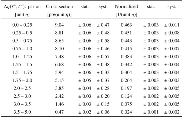
Table 3: Summary of the parton-level absolute and normalised differential cross-sections as a function of Δ𝜂(ℓ+, ℓ−), with statistical and systematic uncertainties in each bin.

Δ𝜂(ℓ+, ℓ−): parton _{Cross-section} _stat. _syst. _Normalised _stat. _syst.

[unit 𝜂] [pb/(unit 𝜂)] [1/(unit 𝜂)]

0.0 – 0.25 9.04 ± 0.06 ± 0.47 0.463 ± 0.003 ± 0.011 0.25 – 0.5 8.81 ± 0.06 ± 0.48 0.451 ± 0.003 ± 0.008 0.5 – 0.75 8.65 ± 0.06 ± 0.58 0.443 ± 0.003 ± 0.004 0.75 – 1.0 8.10 ± 0.06 ± 0.46 0.415 ± 0.003 ± 0.007 1.0 – 1.25 7.48 ± 0.06 ± 0.57 0.383 ± 0.003 ± 0.007 1.25 – 1.5 6.68 ± 0.06 ± 0.38 0.342 ± 0.003 ± 0.004 1.5 – 1.75 5.94 ± 0.06 ± 0.33 0.304 ± 0.003 ± 0.004 1.75 – 2.0 5.15 ± 0.05 ± 0.37 0.264 ± 0.003 ± 0.003 2.0 – 2.5 3.85 ± 0.04 ± 0.28 0.197 ± 0.002 ± 0.005 2.5 – 3.0 2.42 ± 0.03 ± 0.20 0.124 ± 0.002 ± 0.005 3.0 – 3.5 1.46 ± 0.03 ± 0.15 0.075 ± 0.002 ± 0.005 3.5 – 5.0 0.47 ± 0.02 ± 0.06 0.024 ± 0.001 ± 0.002 𝑚_𝑡 ¯

𝑡 range. In all regions of invariant mass, the systematic uncertainties arising from the modelling of the 𝑡 ¯𝑡

and jets are dominant, with statistical uncertainties on the data becoming more important at higher values of invariant mass. In the lowest region of invariant mass, the various NLO predictions differ from each other and from the data. In the other regions of 𝑚𝑡_¯𝑡the differences are less pronounced and agree within

the uncertainties.

The unfolded absolute and normalised particle-level cross-sections for Δ𝜙 and Δ𝜂 are presented in Figure10

and the overall data–MC agreement is very close to that observed at parton level. As with the parton-level results, the normalised uncertainties are significantly smaller than the absolute uncertainties, and signal modelling uncertainties are dominant. The size of the overall uncertainties are similar between fiducial particle and full phase-space parton level for the normalised cross-sections, indicating that the extrapolation to the full phase-space that is modelled by the NLO generators used in the parton-level results is not detrimental.

(23)

] π [rad/ π )/ -,l + (l φ ∆ Parton-level 0 0.1 0.2 0.3 0.4 0.5 0.6 0.7 0.8 0.9 1

Fractional uncertainty size [%]

20 − 15 − 10 − 5 − 0 5 10 15 20 Background Lepton

Luminosity and pileup

miss T

Jet, b-tagging and E modelling t t Stat. Syst. ⊕ Stat. ATLAS -1 = 13 TeV, 36.1 fb s Absolute cross-section (a) ) -,l + (l η ∆ Parton-level 0 0.5 1 1.5 2 2.5 3 3.5 4 4.5 5

20 − 15 − 10 − 5 − 0 5 10 15 20 Background Lepton

miss T

Jet, b-tagging and E modelling t t Stat. Syst. ⊕ Stat. ATLAS -1 = 13 TeV, 36.1 fb s Absolute cross-section (b) ] π [rad/ π )/ -,l + (l φ ∆ Parton-level 0 0.1 0.2 0.3 0.4 0.5 0.6 0.7 0.8 0.9 1

6 − 4 − 2 − 0 2 4 Background Lepton

miss T

Jet, b-tagging and E modelling t t Stat. Syst. ⊕ Stat. ATLAS -1 = 13 TeV, 36.1 fb s Normalised cross-section (c) ) -,l + (l η ∆ Parton-level 0 0.5 1 1.5 2 2.5 3 3.5 4 4.5 5

10 − 5 − 0 5 10 Background Lepton

miss T

Jet, b-tagging and E modelling t t Stat. Syst. ⊕ Stat. ATLAS -1 = 13 TeV, 36.1 fb s Normalised cross-section (d)

Figure 7: Systematic uncertainties for the parton-level differential cross-sections: (top), absolute (a) Δ𝜙 and (b) Δ𝜂 and (bottom), normalised (c) Δ𝜙 and (d) Δ𝜂. The 𝑡 ¯𝑡 modelling uncertainties refer to the contributions from the NLO matrix-element generator (“Generator”), the PS algorithm (“Shower”) and the variation of initial- and final-state radiation (“Radiation”).

(24)

Table 4: Summary of the parton-level absolute and normalised differential cross-sections as a function of Δ𝜙(ℓ+, ℓ−) in four regions of 𝑚𝑡𝑡_¯, with statistical and systematic uncertainties in each bin.

Δ𝜙(ℓ+, ℓ−): parton _{Cross-section} _stat. _syst. _Normalised _stat. _syst.

[rad/𝜋] [pb/(rad/𝜋)] [1/(rad/𝜋)]

𝑚_𝑡 ¯ 𝑡 < 450 GeV 0.0 – 0.2 8.99 ± 0.15 ± 0.71 1.099 ± 0.016 ± 0.035 0.2 – 0.4 8.73 ± 0.14 ± 0.71 1.068 ± 0.015 ± 0.031 0.4 – 0.6 8.25 ± 0.13 ± 0.66 1.009 ± 0.014 ± 0.028 0.6 – 0.8 7.89 ± 0.12 ± 0.60 0.965 ± 0.014 ± 0.024 0.8 – 1.0 7.03 ± 0.12 ± 0.52 0.860 ± 0.013 ± 0.039 450 ≤ 𝑚𝑡𝑡_¯< 550 GeV 0.0 – 0.3 4.10 ± 0.08 ± 0.39 0.781 ± 0.012 ± 0.032 0.3 – 0.6 5.17 ± 0.07 ± 0.40 0.986 ± 0.011 ± 0.031 0.6 – 0.8 5.92 ± 0.08 ± 0.56 1.128 ± 0.014 ± 0.034 0.8 – 1.0 6.42 ± 0.08 ± 0.59 1.223 ± 0.015 ± 0.024 550 ≤ 𝑚𝑡𝑡_¯< 800 GeV 0.0 – 0.4 2.91 ± 0.07 ± 0.32 0.665 ± 0.013 ± 0.024 0.4 – 0.6 4.08 ± 0.10 ± 0.47 0.932 ± 0.020 ± 0.049 0.6 – 0.8 5.42 ± 0.09 ± 0.52 1.237 ± 0.019 ± 0.055 0.8 – 1.0 6.57 ± 0.09 ± 0.65 1.500 ± 0.020 ± 0.031 𝑚_𝑡 ¯ 𝑡 ≥ 800 GeV 0.0 – 0.8 0.99 ± 0.03 ± 0.12 0.771 ± 0.012 ± 0.028 0.8 – 1.0 2.46 ± 0.07 ± 0.27 1.917 ± 0.046 ± 0.105