HAL Id: lirmm-01239175
https://hal-lirmm.ccsd.cnrs.fr/lirmm-01239175
Submitted on 7 Dec 2015
HAL is a multi-disciplinary open access
archive for the deposit and dissemination of sci-entific research documents, whether they are pub-lished or not. The documents may come from teaching and research institutions in France or
L’archive ouverte pluridisciplinaire HAL, est destinée au dépôt et à la diffusion de documents scientifiques de niveau recherche, publiés ou non, émanant des établissements d’enseignement et de recherche français ou étrangers, des laboratoires
Spatio-temporal data classification through
multidimensional sequential patterns: Application to
crop mapping in complex landscape
Yoann Pitarch, Dino Ienco, Elodie Vintrou, Agnès Bégué, Anne Laurent,
Pascal Poncelet, Michel Sala, Maguelonne Teisseire
To cite this version:
Yoann Pitarch, Dino Ienco, Elodie Vintrou, Agnès Bégué, Anne Laurent, et al.. Spatio-temporal data classification through multidimensional sequential patterns: Application to crop mapping in complex landscape. Engineering Applications of Artificial Intelligence, Elsevier, 2015, 37, pp.91-102. �10.1016/j.engappai.2014.09.001�. �lirmm-01239175�
Spatio-Temporal Data Classification Through
multidimensional Sequential Patterns: Application to
Crop Mapping in Complex Landscape
Yoann Pitarcha, Dino Iencoc,d, Elodie Vintroub,d, Agn`es B´egu´eb,d, Anne Laurente, Pascal Poncelete, Michel Salae, Maguelonne Teisseirec,d
aIRIT, Toulouse , France bCIRAD
cIrstea
dUMR TETIS - 500 rue Jean-Fran¸cois Breton, 34093 Montpellier, France eLIRMM - CNRS - UM2
Abstract
The main use of satellite imagery concerns the process of the spectral and spatial dimensions of the data. However, to extract useful information, the temporal dimension also has to be accounted for which increases the complex-ity of the problem. For this reason, there is a need for suitable data mining techniques for this source of data. In this work, we developed a data mining methodology to extract multidimensional sequential patterns to characterize temporal behaviors. We then used the extracted multidimensional sequences to build a classifier, and show how the patterns help to distinguish between the classes. We evaluated our technique using a real-world dataset containing information about land use in Mali (West Africa) to automatically recognize if an area is cultivated or not.
Keywords: Knowledge Discovery, Data Mining, MODIS Images, Remote Sensing, Land Cover
1. Introduction
This work was motivated by a real-world problem in which the final goal is to monitor areas that are not easy to access in order to perform food risk analysis. The northern fringe of sub-Saharan Africa (Sahel belt) is consid-ered to be particularly vulnerable to climate variability and change, which is
why food security remains a major issue in this region [1]. One of the pre-liminary stages necessary for analyzing climate variabilities on agriculture is a reliable estimation of the cultivated land at a national scale. To perform this task, we need to know whether data from several sources (e.g. field surveys, climate, satellite images) can provide a correct assessment of the distribution of cultivated land at a national scale. Although data from satel-lite images are very useful for monitoring land surface, the large quantity of spatio-spectro-temporal measurements stored by the instruments limits the usefulness as sources of information. In recent years, research on spatio-temporal databases has consequently increased alongside research on mining such data [2].
In our analysis, the main problem is to combine heterogeneous sources of information (temporal and static information) to exploit the full set of di-mensions without losing information. To this end, we first need to combine multidimensional temporal and static data. Second, we need a model from which the analyst can easily obtain a clear explanation, since, many previous models are black box models that do not provide a useful explanation for the classification [3].
We thus developed a data mining methodology to extract relevant multi-dimensional sequential patterns from both static descriptions and temporal behaviors.
In data mining literature the term multidimensional is used as a synonym for multi-attribute data, that, instead is commonly employed by researchers in statistics. In the rest of the paper we mainly use multidimensional as the proposed approach comes from the data mining field.
In our scenario, multidimensional (or multi-attribute) temporal measure-ments are obtained from moderate resolution remote sensing images. In the second step, we exploit the acquired knowledge (in terms of sequential patterns) to build a classifier to distinguish between cultivated and non-cultivated areas. Classification techniques based on frequent patterns have been adopted in [4, 5]. Nevertheless, since these approaches are based on association rules, the temporal aspect is not taken into account within the classification rules. One of our originality is to propose a sequential rules-based approach. We applied our model to a real-world dataset from Mali, a representative country of the African Sahel Belt, in which monitoring crop production is a major issue.
In particular, the focus of our analysis is devoted to manage and exploit the temporal dimension of the data while we did not deal with the spatial one. This choice is motivated by the kind of data we analyzed in which the temporal aspect play the main role. In the case the most important dimension of the problem is the spatial one, we refer the interested reader to other techniques explicitly designed to cope with spatial correlations among the data [6].
The main contributions of our work are:
• the management of static and dynamic dimensions of temporal data; • an heuristic approach to filter out irrelevant static dimensions;
• a model where the rules of the classifier are available for detailed in-spection by the analyst.
The reason why, for our study, we adopt multidimensional sequential pat-terns instead of standard machine learning approaches (such as decision trees, support vector machine [7]) is the capacity of these techniques to capture temporal correlation among data. Standard machine learning approaches mainly work on static data and they are not able to intelligently manage this important dimension of analysis.
The proposed approach is an extension of a preliminary work focused on the pattern extraction [8].
The paper is organized as follows: Section 2 supplies problem and pre-liminaries definitions, in Section 3 we introduces a running example. We describe our approach in Section 4. Section 5 describes the satellite and ground dataset we used for our analysis. In Section 6 we present results of our experiments. In Section 7 we give a brief overview of the state of the art. Finally, in Section 8 we conclude.
2. Problem Definition and Preliminaries
In this section, we present the concepts and definitions concerning mul-tidimensional sequential patterns that were inspired by the notations intro-duced in [9]. For each table defined in the set of dimensions D, we consider a partition of D into three sets: Dt for the temporal dimension, DA for the analysis dimensions and DR for the reference dimension. Each tuple c = (d1, . . . , dn), with n the number of dimensions, can thus be denoted
c = (r, a, t) with r the restriction on DR, a the restriction on DA and t the restriction on Dt. We first provide an example to illustrate subsequent definitions.
Example 1. Let D = {AId, A1, A2, A3, AT} be a 5-set of dimensions such that Dt = {AT}, DR = {AId} and DA = {A1, A2, A3}. Table 1 shows some tuples from D. Following the aforementioned notations, the first tuple c1 = (1, 1, a11, a22, a31) can be rewritten into c1 = (r1, a1, t1) with r1 = (1), a1 = (a11, a22, a31) and t1 = (1). AId AT A1 A2 A3 1 1 a11 a22 a32 1 2 a12 a22 a31 1 3 a11 a21 a31 2 1 a12 a21 a32 2 2 a11 a22 a31 3 1 a11 a22 a31
Table 1: An example of table, T .
Definition 1. (Multidimensional Item) A multidimensional item e defined on DA= {D1, . . . , Dm} is a tuple e = (d1, ..., dm) such that ∀k ∈ [1, m] , dk ∈ Dom(Dk).
Definition 2. (Multidimensional Sequence) A multidimensional sequence S defined on DA = {D1, . . . , Dm} is an ordered non empty list of multidimen-sional items S = he1, . . . , eli where ∀j ∈ [1, l], ej is a multidimensional item defined on DA.
Example 2. Assuming DA = {A1, A2, A3}, two possible multidimensional items are e1 = (a11, a22, a32) and e2 = (a12, a22, a32), and S1 = he1, e2i is a multidimensional sequence.
Remark 1. In the original framework of sequential patterns [10], a sequence is defined as an ordered non empty list of itemsets where an itemset is a non-empty set of items. However, given the scope of this paper, we only consider sequences of items since at each date, one and only one item can occur for each identifier.
An identifier is said to support a sequence if a set of tuples containing the items satisfying the temporal constraints can be found. Given a table T , the set of all tuples in T with the same restriction r over DR is said to be a block. Each block B is identified by r. Given a total order on the tem-poral dimension, each block is therefore associated with a multidimensional sequence. and we denote BT ,DR the set of all blocks that can be built up from
table T . The set DR identifies the blocks of the database to be considered when computing supports. The support of a sequence is the proportion of blocks embedding it.
Definition 3. (Tuple Definition) An identifier r ∈ Dom(DR) supports a sequence S = he1, . . . , eli if ∀j ∈ 1 . . . l, ∃dj ∈ Dom(Dt), ∃t = (r, ej, dj) ∈ T where d1 < d2 < . . . < dl.
Definition 4. (Sequence Support) Let DR be the reference dimensions and T a table partitioned into the set of blocks BT ,DR. The support of a sequence
s is defined by:
support(s) = |{B∈BT ,DR | s is included in B}||B
T ,DR|
Definition 5. (Frequent Sequence) Let minSupp ∈ [0, 1] be a minimum user-defined support value. A sequence S is said to be frequent if support(S) ≥ minSupp.
Example 3. Let us consider B1, the block associated with TId = 1. This block is composed by the first three tuples in D. Hence, the multidimen-sional sequence SB1 = h(a11, a22, a32)(a12, a22, a31)(a11, a21, a31)i naturally
re-flects the temporal variations on the analysis dimension values of B1. Now, let us consider the sequences S = h(a11, a22, a32)(a11, a21, a31)i and S0 = h(a11, a21, a31)(a11, a22, a32)i. SB1supports S but not S
0. The support of S is 0.5 since it is only supported by SB1. Assuming minSupp = 0.3, S will be
considered as a frequent multidimensional sequence.
Considering the aforementioned definitions, an item can only be retrieved if there is a frequent tuple of values from domains of DA containing it. For instance, it could be that neither (a11, a22, a32) nor (a11, a22, a31) is frequent whereas the value a11and even a22are frequent. Thus, [9] introduces the joker value ∗. In this case, we consider (a11, a22, ∗) which is said to be jokerized. A jokerized item contains at least one specified analysis dimension. It contains a ∗ only if no specific value from the domain can be set. A jokerized sequence is a sequence containing at least one jokerized item.
Definition 6. (Jokerized Item) Let e = (d1, . . . , dm) a multidimensional item. We denote by e[di/δ] the replacement in e of di by δ. e is said to
be a jokerized multidimensional item if: 1. ∀i ∈ [1, m] , di ∈ Dom(Di) ∪ {∗}, 2. ∃i ∈ [1, m]such that di 6= ∗,
3. and ∀di = ∗, @δ ∈ Dom(Di) such that e[di/δ] is frequent.
Example 4. Let us assume minSupp = 1. Under this constraint, neither I1 = (a11, a22, a32) nor I2 = (a11, a22, a31) is frequent. Indeed, support(I1) =
1
3 and support(I2) = 2
3. However, if we now consider the jokerized item I3 = (a11, a22, ∗), then such item is frequent with support equals 1.
3. Motivating Example
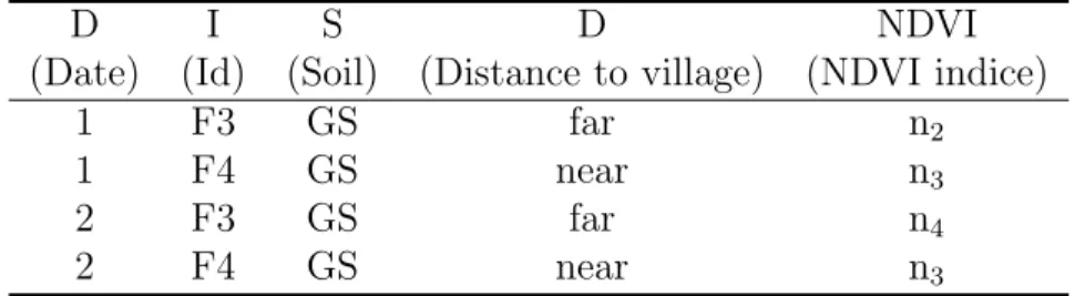
Despite our proposed framework is generic enough to deal with any kind of static and dynamic data, we illustrate our approach through the crop mapping perspective. We thus consider the following scenario that will be used throughout the paper as a running example. Let us consider a relational table T in which N DV I values per field are stored. We assume that T is defined over six dimensions (or attributes) as shown in Table 2. The dimension Dt is the date of statements and we consider two dates, denoted 1 and 2. The I dimension is associated to the field identifier and we consider 4 different fields denoted F 1, F 2, F 3 and F 4. The dimension C is the crop type and we consider two discretized values, denoted F P (food-producing) and N F P (non food-producing). The dimension S represents the soil type whose values can be GS (gravelly soils), SL (sandy loam) and CL (clay loam). The dimension DV is the distance from the field concerned to the nearest village and we consider two discretized values, denoted near and far. The dimension N DV I stands for the N DV I value associated with each field at each timestamp and we consider 4 abstract values n1, n2, n3 and n4 for this example. We consider five sets of dimensions as follows: (i) the dimension Dt representing the date, (ii) the dimension I representing the identifier, (iii) the dimensions S and DV , that we call static dimensions since they do not change over time or descriptors (values of these dimensions associated with a given field do not change over time), (iv) the dimension N DV I, that we call dynamic dimension or indicators (values of these dimensions associated with a given field do evolve over time) and (v) the dimension C that we call
class. For instance, the first tuple of T (Table 2) means that field 1 is a food-producing crop composed of soil CL, near a village and that, at date 1, the N DV I value was n1. Observing the static attribute values of each class in more detail, some comments should be made. First, food-producing crops are always located near the village whereas soil composition changes. Similarly, non food-producing crops are always cultivated on GS whereas the distance to the nearest village changes. A first interpretation of these comments is that the dimension DV appears to be decisive in identifying food-producing crops whereas the dimension S appears to be decisive in identifying non food-producing crops. Consequently, it is relevant to only consider decisive dimensions of each crop when mining representative rules. Once static dimensions have been filtered, the dynamic dimension (N DV I) is considered in order to mine sequential patterns that characterize crops. Let us suppose that we are looking for sequences that are verified by all the crops in a given class. Under this condition, the pattern h(near, n1)(near, n2)i (meaning that fields located near a village and where the N DV I statement are n1 at a certain date and n2 after) characterizes the food-producing crops and the pattern h(GS, n3)i characterizes the non food-producing crops. It should be noted that the representative rules of each class can be composed of values of different dimensions. In the rest of this paper, we describe the method used to determine the decisive attributes of each class and how table T is subdivided and mined to obtain representative rules for each class.
D I C S DV NDVI
(Date) (Id) (Crop) (Soil) (Distance to village) (NDVI value)
1 F1 FP CL near n1 1 F2 FP SL near n1 1 F3 NFP GS far n2 1 F4 NFP GS near n3 2 F1 FP CL near n2 2 F2 FP SL near n2 2 F3 NFP GS far n4 2 F4 NFP GS near n3 Table 2: Table T
4. Method 4.1. Overview
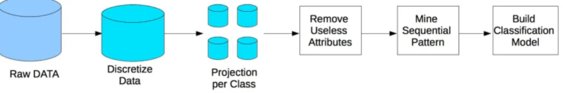
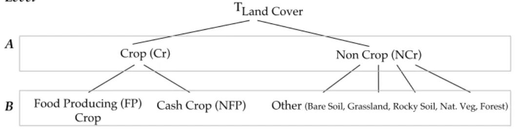
In this study, our aim was to discover and use representative rules in order to characterize crop classes. First we propose a four-step method to discover representative rules for each class, then we combine these rules to build a classifier to distinguish between crop classes. It should be noted that the crop class depends on the user-defined interest level of the crop hierarchy shown in Figure 3. For instance, assuming that the user would like to discover representative rules for classes in the second level of the hierarchy, the set of classes will be {food-producing,non food-producing, other }. The four steps to discover representative rules are illustrated in Figure 1 and are detailled here:
Figure 1: Overall schema of the proposed methodology
1. The raw database pretreatment. During this step, two actions are performed. First, since the raw database stores crops at the lowest level of the hierarchy, these attributes values must be rewritten to match the user-defined interest level. Second, sequential pattern mining aims to discover frequent relations in a database but is not suitable for mining numerical attributes (e.g., distance to village, NDVI value) due to the huge definition domain of such attributes. Consequently, numerical attributes are discretized to improve the sequential pattern mining step. 2. The building of projected databases. Since we would like to obtain representative rules for each class, the pretreated database is projected on the different class values.
3. The decisive attribute computation. During this step, a search is performed on each projected database in order to find and delete non-decisive static attributes. Intuitively, a static attribute is said to be non-decisive if none of its value allows the class to be character-ized. More precisely, we guarantee that if there is no value of a static
attribute in at least minSupp% of the projected database, the represen-tative rules associated with this class will never contain specific values of this static attribute. Consequently, it is a waste of time to consider it in the rest of the process and this attribute is discarded from the projected database.
4. The sequential pattern mining. Once the projected databases have been cleaned, the algorithm M2SP [9] is applied on each database. We obtain a set of frequent patterns for each class.
Once the representative rules for each class have been extracted, we combine them to build a classifier.
These steps are detailed in the following subsections.
4.2. Database Pretreatment and Projections
The first treatment is rewriting the database to match the values of the crop attributes to the user-defined interest level. This is motivated by two reasons. First, mining representative rules for precise crop values is not consistent. Consequently, crop attribute values must be rewritten, at least to the level of granularity above. Second, since the hierarchy is com-posed of two workable levels of granularity, it is interesting to allow the user to choose which level to explore. To this end, a user-defined parame-ter, Level, is introduced to specify which level of granularity to mine. As a result, rules representing different generalized classes can be compared. Table 2 gives an example of database rewriting in which crop attribute val-ues have already been generalized to the second level of granularity (i.e., Dom(Crop) = {F P, N F P }).
The second pretreatment is the discretization of numerical attributes. This is motivated by the use of the sequential pattern technique to mine representative rules. Indeed, sequential pattern algorithms aim to discover frequent relations among the fields belonging to the same class. When dealing with numerical attributes, two values can be considered as different items even if they are very close. For instance, let us consider that the distance to the nearest village is 200 meters for field 1 and 205 meters for field 2. Without discretization, these two distances would have been considered as different items by the M2SP algorithm even if they are semantically close. In our application, numerous attributes are numerical, so discretization is required. Numerous discretization techniques can be found in the literature [11]. Section 6 details the technique used for each numerical attribute.
Once the database has been pretreated, projection on each crop attribute value is performed. This is motivated by the fact that we would like to discover representative rules for each class. An intuitive way to achieve this goal is to subdivide the pretreated table into smaller ones associated with each class. Tables 3 and 4 show the result for our running example.
D I S D NDVI
(Date) (Id) (Soil) (Distance to village) (NDVI indice)
1 F1 CL near n1
1 F2 SL near n1
2 F1 CL near n2
2 F2 SL near n2
Table 3: TF P, the F P projected table
D I S D NDVI
(Date) (Id) (Soil) (Distance to village) (NDVI indice)
1 F3 GS far n2
1 F4 GS near n3
2 F3 GS far n4
2 F4 GS near n3
Table 4: TN F P, the N F P projected table
4.3. Dimensionality Reduction
Once the projected databases have been built, a search is performed on the static attributes of each database to identify unnecessary static at-tributes. Intuitively, if the values of a static attribute change a lot, the attribute is not really characteristic of this class, and can be deleted from the projected class. The main advantage of such a strategy is to reduce the search space during the sequential pattern mining step. Indeed, it is empir-ically shown in [9] that the number of dimensions exponentially influences both memory consumption and extraction time. Whereas traditional appli-cations often deal with only a few analysis dimensions, this point can be very
problematic in our context since the number of both static and dynamic di-mensions can be high. For instance, the experimental results presented in Section 6 concern up to 12 dimensions. Traditional multidimensional se-quential pattern approaches cannot efficiently deal with such a number of analysis dimensions. Moreover, aside from performance considerations, it is important to note that the higher the number of dimensions, the higher the number of extracted patterns. Since the extracted patterns will be exploited by experts, reducing the dimensionality without loss of expressivity is very useful to improve the results of the analytical step.
To perform such a dimensionality reduction, we proceed as follows. Let minSupp be the user-defined parameter used during the sequential pattern mining step, let Ti be a projected database and Dj ∈ Ti be one the static dimension in Ti. It can be easily proved that if there is no value of Dj appearing at least minSupp × |Ti| tuples in Ti (where |Ti| is the size of Ti), no sequential pattern can be extracted from Ti where a value of Dj appears. If so, the dimension Dj is considered as unnecessary and is thus deleted from Ti. A direct corollary of this property is that if an attribute is retained, there will be at least one sequential pattern containing a value of Dj. To illustrate this affirmation, let us consider, TF P, the projected database presented in Table 3 and minSupp = 1. The two static attributes are D and S. Regarding the D attribute, all the tuples share the same value (near). This attribute is considered as useful for the next step and is thus retained. Let us now consider the S attribute. Here, no value satisfies the minSupp condition. As a consequence, S is deleted from this table. To check the consequence of such a strategy, let us consider, SPF P, the set of the multidimensional sequential patterns extracted from TF P where minSupp = 1, Dt= D, DR= I and DA = {C, S, N DV I} (i.e., all the static and dynamic attributes are considered). Under these conditions, SPF P = {h(∗, near, n1)i, h(∗, near, n1)(∗, near, n2)i}. It rapidly becomes obvious that D occurs in SPF P but not S.
It is interesting to observe that the set of useful attributes of each class can differ. As a consequence, independently of the values of these attributes, the attributes themselves can be representative of one class. For instance, when applying the dimensionality reduction technique to TN F P described above (see Table 4), S, not D, is retained.
4.4. Mining Representative Rules
Once unnecessary attributes have been deleted, the M2SP algorithm is applied on each projected and cleaned database Ti such that minSupp is the same as defined during the previous step, Dt = D, DR= I and DA is com-posed of the static attributes and dynamic attributes retained. We denote SPTi the set of sequential patterns extracted from Ti. For instance
consid-ering TF P and minSupp = 1, h(near, n1)(near, n2)i is a frequent sequence meaning that NDVI values equal n1 and then n2 is a frequent behavior for fields under food-producing crops located near a village.
4.5. The Classification Model
In this step we combine multidimensional sequential patterns to obtain a global classification model. We name our method MSPC (Multidimensional Sequential Pattern Classifier). The general procedure is presented in algo-rithm 1. The algoalgo-rithm MSPC takes as input the training data Dtrain over which it learns the model, the test data Dtest that represents the set of new objects to classify, the parameter k that specifies the number of rules per ob-ject to use to classify it and the support threshold suppt used to extract the sequential patterns per class. The suppt is the same for all the classes. The MSPC (Algorithm 1) starts retrieving the set of classes C using the function classes over the training data Dtr. As a second step it projects the whole training dataset over only the sequences belonging to a class c, this operation is done by the function classP rojection. Then the algorithm extracts the set of rules to use in the classification process. To do this, it calls the pro-cedure extractRules. This propro-cedure mines the frequent multidimensional sequential patterns per class.
In Algorithm 3 the pseudo-code of this approach is supplied. It builds the set L of rules used for the classification. A rule is a triple (s, w, c) where s is a multidimensional sequential pattern and w stands for the weight of the rule for the class c. The concept of rules is different by the concept of sequential pattern, in particular a sequential pattern could appear in more than one class while a rule is specific for each class. The weight w differ-entiates the sequential patterns and it could be seen as the strength of the specific sequential pattern s for the class c. Given a class c and a sequential pattern s we compute the weight w as follows:
w = getSupp(s, Dc) getSupp(s, D)
The function getSupp returns the support (the number of sequences that support a sequential pattern) in the specified dataset. w has a value greater than 1 if the support in Dc (sequences in class c) is greater than the support in the whole dataset (sequences in the training set Dtrain). In this case we can assume that the presence of the pattern in class c is significant w.r.t. the whole dataset. When the weight is equal to 1, the support statistic in both the class c and the dataset is the same. If the value is less than 1, we can assume that the presence of the pattern in the class is less significant. In this paper we use the notation . to access each element of the rule. The MSPC algorithm uses the set of rules L to classify each test instance. To do this it employs the classif yInstance function (Algorithm 2).
It takes as input the instance to classify x, the set of rules L, the number of rules to use k and the set of classes C. First it extracts the order set of rules Lx from L that are supported by x (x supports the sequence s associated to the rule in L). The set is ordered in decreasing order w.r.t. the weight w. From Lx the algorithm retains only the first k rules, we call this ordered set Lk
x. The final classification for the object x is given by the following formula: arg max
c∈C X l∈Lc,kx
l.w · I{l.c == c}
where l.w and l.c are respectively the weight and the class of the rule l, I{l.c == c} is the indicator function and it is equals to 1 if the argument is true otherwise it returns 0. Practically, we choose, as final label, the class that maximizes the sum of the weight in the set of top-K supported rules. This process is performed for all the objects in Dtest and the final classification is returned by the algorithm. The classification is used to compute any evaluation measure to test the performance of the classifier.
Algorithm 1 MSPC(Dtrain, Dtest, k, suppt)
1: C = classes(Dtrain)
2: L = extractRules(Dtrain, suppt, C)
3: predictedValue = ∅
4: for all x ∈ Dtest do
5: predictedValue[x] = classifyInstance( x, L, k, C)
6: end for
Algorithm 2 classifyInstance(x, L, k, C)
1: findClass = ∅
2: Lx = {l|l ∈ L ∧ x supports l.s}
3: Lkx = extractTopK(Lx, k)
4: findClass = arg maxc∈CPl∈Lc,k
x l.w · I{l.c == c}
5: return findClass
Algorithm 3 extractRules(D, suppt, C)
1: L = ∅ 2: for all c ∈ C do 3: Dc =classProjection(D, c) 4: S = extractFreqPattern(Dc, suppt) 5: for all s ∈ S do 6: w = getSupp(s,Dc) getSupp(s,D) 7: L = L ∪ (s, w, c) 8: end for 9: end for 10: return L 4.6. Complexity Analysis
We now provide an analysis of the time complexity of the proposed methodology. It is noteworthy that the first two steps, i.e. data pretreat-ment, projections and dimensionality reduction, can be merged and achieved in linear time on the size of the table T . Indeed, one scan of T is necessary to dispatch each tuple in its appropriated projected table, discretize numer-ical values and count each value. Once this scan has been performed, one has to discard static dimensions in which no item is frequent. The multi-dimensional sequential pattern mining is the most time consuming step of our framework. From a theoretical point of view, enumerating frequent se-quences is NP-hard [12]. However, M2SP performs well on relatively large databases in practice. Indeed, experiment results reported in [9] show that mining multidimensional sequential patterns can be achieved in reasonable time, e.g., it takes around 20 minutes to mine patterns in a database of 25K tuples considering 15 dimensions and minSupp = 0.5. Finally, the time to perform the classification step is logarithmic on the number of extracted rules, denoted by n. Here again, this number is theoretically exponential on the number of dimensions and the definition domain size of each dimension.
However, it is well-known that minSupp constraint can drastically help in reducing the number of mined patterns, i.e., the higher minSupp, the lower the number of patterns. Since we aim at considering only the k most impor-tant rules according to their weight, the n rules can be sorted in logarithmic time. Extracting the k first rules and finding the predicted class is then straightforward.
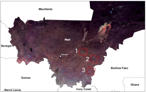
5. Data Description
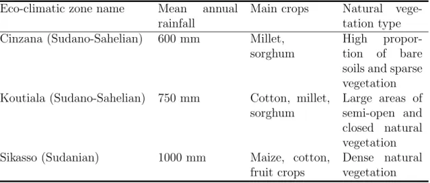
In this project, we used data acquired over 3 sites in southern Mali (Figure 2). Mali is representative of the Sahel Belt, a region where mapping culti-vated areas is still a challenge. First, Sahel is a transition zone between the hyper-arid Sahara in the north and the more humid savannas and woodlands in the south, with specific weather conditions resulting in high regional vari-ability in terms of rainfed agricultural systems (and calendars); second, West African landscapes are complex, with small-scale farming, numerous trees in the fields, and synchronized phenology for crops and natural vegetation due to the rainfall regime [13].
Eco-climatic zone name Mean annual rainfall
Main crops Natural vege-tation type Cinzana (Sudano-Sahelian) 600 mm Millet,
sorghum
High propor-tion of bare soils and sparse vegetation Koutiala (Sudano-Sahelian) 750 mm Cotton, millet,
sorghum
Large areas of semi-open and closed natural vegetation Sikasso (Sudanian) 1000 mm Maize, cotton,
fruit crops
Dense natural vegetation
Table 5: Main characteristics of the three study sites
5.1. Field data
Fields surveys were conducted in Mali during the 2009 and 2010 cropping seasons (from May to November) in order to characterize Sudano-Sahelian
Figure 2: The three study sites in Mali (a color composite MODIS image) - 1: Cinzana, 2: Koutiala ; 3: Sikasso
rural landscapes. Three sites (Cinzana, Koutiala, Sikasso) were selected to sample the main agro-climatic regions of central and southern Mali (Table 5). A total of 744 GPS waypoints were registered and farmers were interviewed. Each waypoint was transformed into a polygon and a land use was attributed to the center of each polygon.
Land Cover! Cash Crop (NFP)! Food Producing (FP) ! Crop! Τ Level! A!
B! Other (Bare Soil, Grassland, Rocky Soil, Nat. Veg, Forest)!
Figure 3: Crop hierarchy: The hierarchical organization of the classes to predict. Level A contains only two classes: Crop, Non Crop while level B refines the previous set of classes adding a specialization (Food Producing Crop, Cash Crop) of the Crop class. The class labels for the data are manually collected by the experts involved in the project during field missions in MALI region.
5.2. External data
Seven static descriptors were also used to characterize the survey points: • soil type
• name of the eco-region
• distance to the nearest village • distance to the nearest river • rainfall
• ethnic group • name of the village
5.3. Image data
MODIS (or Moderate Resolution Imaging Spectroradiometer) [14] is a key instrument aboard the TERRA and AQUA satellites. The NASA Land Process Distributed Active Archive Center (LP DAAC) is the repository for all MODIS data. Among the MODIS products, we selected the ”Vegetation Indices 16-Day L3 Global 250m SIN Grid” temporal syntheses (MOD13Q1). In fact, the quality of MODIS images is affected by atmospheric contami-nation (clouds and aerosols). MODIS images are therefore composited over 8 or 16 days using cloud-screening algorithms and these temporal syntheses were especially useful in our study because of the high probability of cloud cover during the monsoon season in West Africa.
In our study, a set of 12 MODIS 16-day composite normalized difference vegetation index (NDVI) images (MOD13Q1/V005 product) at a resolution of 231.6 m were acquired in 2007 (we selected the best quality composite image out of the two acquire each month) from the NASA LP DAAC. The year 2007 was chosen to overlap with more recent higher resolution data. We assume that the observed classes of land use (Figure 3) remained globally unchanged from 2007 to 2009 (the field surveys were conducted in 2009).
We underline that the proposed data mining framework is not specific to MODIS images but it can be straightforwardly applied on high resolution time series. In our scenario, due to project constraints, the only available images are MODIS ones. From a practical point, considering only low resolu-tion images is not limitaresolu-tion because: i) low resoluresolu-tion images are cheaper or freely available ii) they allow to consider longer and denser time series as they are produced with higher frequency iii) if the results on low resolution im-ages are satisfactory, probably with high resolution imim-ages the performance will improve. These considerations summarize the pragmatic implications to considering as source of information MODIS time series
5.4. Remotely-sensed indices used
Information content in a digital image is expressed by the intensity of each pixel (i.e.,. reflectance or spectral index) and by the spatial arrangement of pixels (texture) in the image.
• The Normalized Difference Vegetation Index, or NDVI, is one of the most successful indices to simply and rapidly identify vegetated areas [15] and their ”condition”, providing a crude estimate of vege-tation health. Based on the spectral contrast that exists between soil
and green vegetation in the RED and NIR spectral bands (intensity), commun bands used in the Earth Observation Systems, NDVI is used as a proxy of plant biomass and fractionnal vegetation cover.
N DV I = N IR − RED N IR + RED
where RED and NIR stand for the spectral reflectance measurements acquired in the red and near-infrared regions, respectively. In general, NDVI values range from -1.0 to 1.0, with negative values indicating clouds and water, positive values near zero indicating bare soil, and higher positive values of NDVI ranging from sparse vegetation (0.1 -0.5) to dense green vegetation (0.6 and above). Furthermore, different land covers exhibit distinctive seasonal patterns of variation in NDVI. Crops generally have a distinct growing season and period of peak greenness, which allows them to be distinguished from other types of land cover.
• Texture analysis is also an important contributor to scene information extraction. The majority of image classification procedures, particu-larly those in operational use, rely on spectral intensity characteristics alone and thus ignore the spatial information contained in the image. Textural algorithms, however, attempt to measure image texture by quantifying the distinctive spatial and spectral relationships between neighboring pixels. Numerous texture algorithms have been developed in response to the need to extract information based on the spatial arrangement of data in digital images. Statistical approaches, such as those developed by [16] make use of gray-level probability density functions, which are generally computed as the conditional joint prob-ability of pairs of pixel gray levels in a local area of the image. In this study, we used four Haralick textural indices [17] calculated on the MODIS time-series: variance, homogeneity, contrast and dissimilarity. The Haralick textural features describe the spatial distribution of gray values and the frequency of one gray tone appearing with another gray tone in a specified distance and at a specified angle. The generation of these indices is based on different orientations of pairs of pixels, with a specific angle (horizontal, diagonal, vertical, co-diagonal) and distance, called patterns. We determined empirically a pattern size of 15 pixels
for MODIS, which is the smallest patch repeated in different directions and at different distances.
6. Experiment Study
In this section, we describe the experiments performed to evaluate the feasibility and efficiency of our approach. Throughout the experiments, we answer the following questions that are inherent to efficiency issues: Does the dimensionality reduction technique allow unnecessary static attributes to be deleted without losing information? Does the mining process allow discrimi-nating patterns to be discovered in each class ? Does the texture data allow better extraction of discriminating patterns than only considering NDVI val-ues? Does the extracted pattern enable a good classifier to be built? Is the classification process affected by the support threshold? Which dimensions allow the best classification? The experiments were performed on a In-tel(R) Xeon(R) CPU E5450 @ 3.00GHz with 2GB of main memory, running Ubuntu 9.04. The methods were written in Java 1.6. We first describe the protocol and then present and discuss our results. In order to evaluate the performance of our method we use the F-Measure. Finally, we discuss about the genericity of the proposed framework.
6.1. Protocol
The method was evaluated on the dataset described in Section 5. This dataset contains 744 distinct fields, and a MODIS time-series of length 12 was associated with each field. The seven static dimensions and the five dynamic dimensions (NDVI, variance, homogeneity, contrast and dissimilar-ity) were the same as described in Section 5. As mentioned in Section 4, a discretization step is necessary to efficiently mine frequent patterns. The following discretization methods were used:
• Equi-Width technique (the generated intervals have the same width) was used for distance to village, and for distance to river attributes. • Equi-Depth technique (the generated intervals are the same size) was
used for the other numerical attributes.
The motivation behind these choices are the following. First, these two techniques are very well known and extensively used in data mining ap-proaches where numerical attributes need to be converted into categorical
attributes, i.e., intervals. Then, we experimentally verified that this setting offers the best experimental results. Interested readers could refer to a recent survey on discretization techniques in [18].
Two sets of classes were used in this experiment. The first set of classes, denoted B, aims to discover patterns enabling the distinction between food-producing crops (FP), non food-food-producing crops (NFP) and non crops (OTHER). The second set of classes, denoted A, aims to discover patterns enabling the distinction of more general classes, i.e., crops (Cr) and non crops (N Cr).
To evaluate the impact of texture data on the extraction of discriminating patterns, we consider a first configuration, denoted Def ault, in which all the dynamic attributes were used. Conversely, the configuration denoted N DV I was only composed of NDVI values as dynamic attributes.
Three experimental results are presented and discussed in this section: 1. The first experiment was performed to evaluate the number of retained
static attributes according to two minSupp values offering representa-tive results.
2. The second experiment was performed to evaluate the number of dis-criminating patterns. Here, disdis-criminating means that a pattern ap-pears in one class but not in the others.
3. The third experiment was performed to observe the discriminating di-mension values according to the two configurations described above. 6.2. Results and Discussion on Patterns
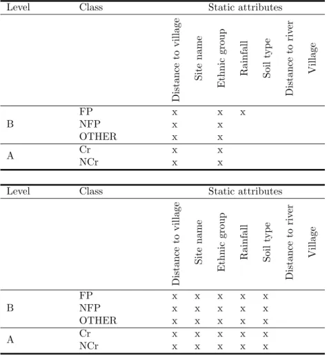
Table 6 shows the retained attributes according to the two sets of classes and two minSupp values. First, it can be seen that the minSupp threshold value had obvious clear impact on this attribute selection. Indeed, when minSupp = 0.5, more than half of the attributes were deleted. It is also interesting to note that the retained attributes per class and set of classes were roughly the same.
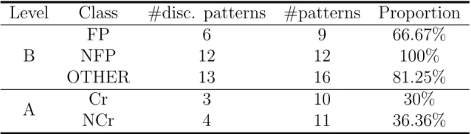
Table 7 shows the proportion of discriminating patterns per class with minSupp = 0.5 and the NDVI configuration. Indeed, even if a pattern was extracted from one class, this is not enough to consider it as discriminating (i.e., since the same pattern can appear in different classes). Thus, queries were formulated to search for patterns that appear in one class and not in any others. Two conclusions can be drawn from this figure. First, considering the set of classes B, most of the extracted patterns are discriminating (even
Level Class Static attributes Distance to village Site name Ethnic group Rainfall Soil typ e Distance to riv er Village B FP x x x NFP x x OTHER x x A Cr x x NCr x x
Level Class Static attributes
Distance to village Site name Ethnic group Rainfall Soil typ e Distance to riv er Village B FP x x x x x NFP x x x x x OTHER x x x x x A Cr x x x x x NCr x x x x x
Table 6: Retained static attributes under default configuration (up: minSupp = 0.5 / down: minSupp = 0.3)
Level Class #disc. patterns #patterns Proportion B FP 6 9 66.67% NFP 12 12 100% OTHER 13 16 81.25% A Cr 3 10 30% NCr 4 11 36.36%
Table 7: Proportion of discriminating patterns per class with minSupp = 0.5 and the NDVI configuration
if the F P class obtained the worst score). Second, finding discriminating patterns on the set of class A is apparently more difficult.
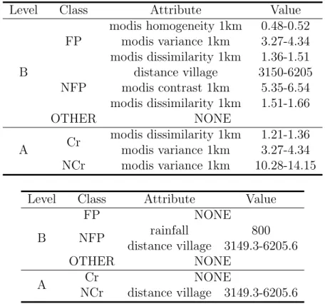
Table 8 shows some representative values of discriminating attributes ac-cording to the two configurations and the two sets of classes. An attribute value is said to be discriminating if it does not appear in a pattern in any other classes. The aim of this experiment is to observe the impact of texture dynamic values on the extracted patterns. Some conclusions can be drawn. First of all, class OT HER does not contain any discriminating values in-dependently of the configuration. Second, a very interesting and promising result is that the default configuration contains many more discriminating values than the NDVI configuration. Moreover, these discriminating values concern the texture attributes. This result reinforces our hypothesis that texture attributes are very useful in automatic landscape recognition.
To conclude the first part of our experiment, we empirically showed that (1) the dimensionality reduction method allows the search space to be re-duced by deleting unnecessary attributes; (2) most of the extracted patterns are discriminating; (3) it appears to be more difficult to distinguish between Cr and N Cr classes than F P , N F P and OT HER classes with our approach and (4) most of the discriminating attribute values concern the texture at-tributes. In the second part of the experiment we used the previously ex-tracted patterns to build the MSPC classifier. We saw that the patterns are able to discriminate between the classes of the problem. For this reason we hypothesize that combining them will enable us to obtain very interesting results from the classification point of view, especially with respect to the problem of distinguishing between Cr and N Cr classes.
Level Class Attribute Value B FP modis homogeneity 1km 0.48-0.52 modis variance 1km 3.27-4.34 modis dissimilarity 1km 1.36-1.51 NFP distance village 3150-6205 modis contrast 1km 5.35-6.54 modis dissimilarity 1km 1.51-1.66 OTHER NONE A Cr modis dissimilarity 1km 1.21-1.36 modis variance 1km 3.27-4.34 NCr modis variance 1km 10.28-14.15
Level Class Attribute Value
B FP NONE NFP rainfall 800 distance village 3149.3-6205.6 OTHER NONE A Cr NONE NCr distance village 3149.3-6205.6
Table 8: Some discriminating dimension values per class with minSupp = 0.3 (top: default config. / bottom: NDVI config.)
6.3. Results and Discussion on Classification
In this section we evaluate the capacity of MSPC to discriminate between Cr and NCr classes, but in fact, it could be applied at any level of the hierarchy in Figure 3. We evaluated the classification results using Precision and Recall for the Cr label. Finally, we combined these two measures using the F-Measure. The Precision is defined as the number of areas correctly assigned to the class Cr divided by the total number of areas assigned to this class (correctly or not). The Recall is the number of areas correctly assigned to the class Cr divided by the number of areas with true label equals Cr. Finally the F-Measure is defined as:
F-Measure = 2 × P recision × Recall P recision + Recall
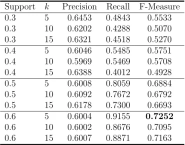
Since sequential pattern mining uses discrete data, we used the equi-width discretization method to discretize the time-series values. For our approach we varied the support threshold from 0.3 to 0.6 and the values of k ranges over the set {5,10,15}. The choice of minimum support threshold values and step size are motivated by the following arguments. First, it is crucial to extract at least one frequent pattern per class. Otherwise, it would lead to the construction of a classifier containing unrepresented class. Thus, we ex-perimentally verified that with a support threshold above 0.6, some classes were not represented. Conversely, setting up the minimum support thresh-old to a very low value does not really make sense in our approach since we only consider the k extracted patterns having the highest score. Second, we experimentally verified that this step size allows to show the most represen-tative results. The choice of k values and step size are motivated by the following arguments. First, considering a very low value for k contradicts the vote-based classification system philosophy. Conversely, setting up the k value to a high value will introduce the selection of noisy patterns, i.e., pat-terns with low supports, in the process and will decrease the performances. Second, similarly to the minimum support step size motivation, we experi-mentally verified that this step size allows to show the most representative results. We also adopted a 10 Fold Cross Validation strategy to test the generalization ability of our approach.
In our comparison, we used the MOD12Q1 V005 as base-line competitor. This product, based on an ensemble classification approach, is widely used in the remote sensing field. The base algorithm is a decision tree [19] and ensemble classifications are estimated using boosting [20]. The results of this
Precision Recall F-Measure 0.63945 0.6578 0.6485
Table 9: Classification results usint the MOD12Q1 V005 base-line product
Support k Precision Recall F-Measure 0.3 5 0.6453 0.4843 0.5533 0.3 10 0.6202 0.4288 0.5070 0.3 15 0.6321 0.4518 0.5270 0.4 5 0.6046 0.5485 0.5751 0.4 10 0.5969 0.5469 0.5708 0.4 15 0.6388 0.4012 0.4928 0.5 5 0.6008 0.8059 0.6884 0.5 10 0.6092 0.7672 0.6792 0.5 15 0.6178 0.7300 0.6693 0.6 5 0.6004 0.9155 0.7252 0.6 10 0.6002 0.8676 0.7095 0.6 15 0.6007 0.8871 0.7163
Table 10: Classification results using all dynamic time-series information
approach are listed in Table 9. Table 10 shows the classification of the Mali dataset using our method. It can be seen that higher F-Measure values were obtained with an increase in the support threshold. This probably happened because, with a low support threshold we also obtain noisy patterns that could influence the whole process. In particular, these noisy patterns could be anomalous patterns that represent particular behavior associated with a particular geographical area, but not are related to the problem of discrim-inating between Crop and Non Crop areas. Compared with the baseline method presented in Table 9, our results were good. In fact with a support equal to 0.5 or 0.6, the classifier gave very good results (a F-Measure greater than 0.70) compared with the baseline approach.
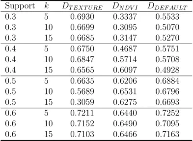
6.3.1. Evaluation of different projections over dynamic dimensions
In this subsection, our aims is to identify the most important source of information to distinguish Crop and Non Crop areas. When we consider dynamic information we have two different groups of information, the first
Support k DT EXT U RE DN DV I DDEF AU LT 0.3 5 0.6930 0.3337 0.5533 0.3 10 0.6699 0.3095 0.5070 0.3 15 0.6685 0.3147 0.5270 0.4 5 0.6750 0.4687 0.5751 0.4 10 0.6847 0.5714 0.5708 0.4 15 0.6565 0.6097 0.4928 0.5 5 0.6635 0.6206 0.6884 0.5 10 0.5689 0.6531 0.6796 0.5 15 0.3059 0.6275 0.6693 0.6 5 0.7211 0.6440 0.7252 0.6 10 0.7152 0.6490 0.7095 0.6 15 0.7103 0.6466 0.7163
Table 11: Classification (F-Measure) results using different projections over dynamic di-mensions
is supplied by the NDVI, and the second is supplied by the four texture indices. For our analysis, from the original dataset, we obtain two different projections that we denote DN DV I and DT EXT U RE. DN DV I is the projection of the original dataset over the static dimensions plus the NDVI time-series while the DT EXT U RE is the projection of the original dataset over the static dimensions plus the four texture time-series. Table 11 shows the F-Measure resulting from the classification process using the different projections over dynamic dimensions. In this comparison, the best results were obtained with the full set of information (0.72 with support equal 0.6 and k equal 5). From this analysis, we can conclude that the most useful information to discriminate between the classes of the problem is supplied by the texture dimensions. This information always produced interesting results and was not affected by changing support values. The worst results were obtained when the classifier used only the NDVI information. From this analysis we can conclude that the texture information plays a very important role in discriminating between Crop and Non Crop areas, while the NDVI dimension mostly affects the quality and the stability of the results.
Support k Equi-Depth Equi-textureWidth 0.3 5 0.5459 0.5533 0.3 10 0.6005 0.5070 0.3 15 0.6609 0.5270 0.4 5 0.6663 0.5751 0.4 10 0.6257 0.5708 0.4 15 0.6262 0.4928 0.5 5 0.4242 0.6884 0.5 10 0.4623 0.680 0.5 15 0.4456 0.6693 0.6 5 0.1252 0.7252 0.6 10 0.2435 0.7095 0.6 15 0.2347 0.7163
Table 12: Classification (F-Measure) results using different projections over dynamic di-mensions
6.3.2. Impact of different discretization over dynamic dimension
In this section we evaluate to what extent the discretization technique used to manage the dimenions of the time-series affects the final results. Table 12 shows part of the results of the experiment.
We observed that the classifier learned with the Equi-Depth discretization was very sensitive to changes in the support threshold. In fact, for low support threshold it gave good quality results, but its performance decreased with an increse in the support threshold. Examining the data in more detail, we observed that the classification using Equi-Depth discretization always obtained good results with respect to the Precision measure but the Recall drastically decreased and as a result, the F-Measure also decreased. This means that the Equi-Depth discretization influences the whole process by increasing the number of false negatives. This increase in the number of false negatives means that the rules will assign nCr label to Cr areas. In the same context we observed that while the performance of the classification decreased with the full set of dimensions, if we used the Equi-Depth discretization combined only with the texture information the results we obtained were of good quality and were very similar to those obtained using Equi-Width discretization. This means that Equi-Depth discretization mainly affects the discriminating ability of the NDVI dimension and consequently reduces
Number Sequential Pattern Weight Class 1 <(distance village=-inf-3149.3,modis ndvi=2182.6-2927.0) 1.074524 Cr
(distance village=-inf-3149.3,modis ndvi=2927.0-3671.5)> 2
<(modis ndvi=2182.6-2927.0,ethnic group=senoufo nanerige)
1.0115681 NCr (modis ndvi=2182.6-2927.0,ethnic group=senoufo nanerige)
(modis ndvi=2927.0-3671.5,ethnic group=senoufo nanerige)>
3 <(modis variance=-inf-7.585,modis contrast=-inf-6.245) 1.03212 Cr (modis variance=-inf-7.585,modis contrast=-inf-6.245)>
Table 13: Example of rules
overall performance.
6.3.3. Low support patterns
We have seen that support influences the performance of the classification step. The aim of this set of experiments was to evaluate the classification performance using a lower support threshold. Usually using a low thresh-old avoid noisy patterns that are shared between all the classes. Instead, in our study we obtained worst results by decreasing the threshold. When the support value we used was too low we observed that the algorithm used infre-quent patterns that could resemble local anomalies or patterns that describe only a particular geographical zone but are not able to describe the over-all difference between Cr and nCr areas. Another interesting observation, from the point of view of our analysis, is that when we used a low support threshold, the classifier learned using only the NDVI projection gave similar or slightly better results to the classifier learned using the full set of dynamic dimensions.
6.3.4. Example of rules
Table 13 lists some examples of rules that we extracted from MSPC. To make the analysis easier we only show the dimensions used and avoid showing the dimensions with no specific value with the ∗ operator. For the same reason, we multiply the value of NDVI by 104 because this helps interpret of the bins obtained by the discretization step.
It can be seen that, using our approach, we were able to take both static and dynamic dimensions into account as shown in rules 1 and 2.
In rule 1, the algorithm uses the combination of a static information (distance village) with a change in the value of NDVI to predict Cr areas. In this rule, the weight or score was greater than 1.
In rule 2, a pattern composed of three multidimensional items, appeared that gave a high score for the NCr. In this rule, static information is always combined with dynamic information. In this particular case, we observed that the NDVI was stable in the first and second multidimensional item, whereas it increased in the third position of this sequence. This phenomenon is closely correlated with the ethnic group and is a good indicator to predict NCr areas.
In rules 3 and 4, the same rule is used to predict both classes but with a different score. In these rules, the two multidimensional items involved in the sequence are always the same. This is still an useful information because it underlines the fact that constant behaviors are also useful to discriminate the two classes.
We also supply the entire set of rules (per class) to remote sensing experts in order to have a qualitative interpretation of them. After some manual in-spection, the experts highlighted that the rules employed in the classification model are coherent with the temporal profile of each class. The interpretabil-ity of the rule set, supplied by our model, is a bonus of of our proposal. 6.4. Genericity of MSPC
In this section, we discuss about the genericity of the framework that has been proposed in this paper. Multidimensional and heterogeneous data are rarely considered as input of classification techniques. Indeed, most of pattern-based classification techniques focus on the sequential behavior and omit to take contextual and external knowledge into account. Though, re-cently, a new trend in the data mining field tries to incorporate expert knowl-edge in the process to improve the result quality [21, 22, 23]. Our approach clearly comes within this scope and we experimentally show that adding as much as available non-sequential information would lead to increase the clas-sification performances. Moreover, thanks to the dimensionality reduction mechanism, we guarantee that no matter the number of additional dimen-sions we consider, the framework will select the most appropriated ones in order to preserve the scalability.
7. Related Work
In literature several sequential pattern mining approaches are proposed to deal with spatio-temporal data. In [24] a method to mine frequent sequential patterns from spatio-temporal data is presented. Given a set of objects that
move together, this strategy extract frequent routes followed by the objects. The mined pattern are constrained to be consecutive w.r.t. the temporal dimension.
A more recent approach that extracts sequential patterns from spatio-temporal events is introduced in [25]. The authors proposed to use an in-dexing structure in order to mine the sequential behavior of events in the data. The final patterns are sequences of events that occur in the same neighborhood area. This kind of approach is useful if the objects to follow slightly change their position while they are equivalent to standard sequential patterns when the followed objects do not move.
In [26, 27, 28, 29] sequential pattern mining methods are employed to extract useful knowledge from Time Series of Satellite Images (TSSI). The interest in these methods used to detect change using satellite images is due to the fact that they are (i) multi-temporal, (ii) robust to noise, (iii) able to handle large volumes of data, and (iv) capable of capturing local changes without the need for prior clustering.
Sequential pattern mining is used to analyze changes in land cover over a 10-month period in a rural area in eastern Romania in [27]. Pattern ex-traction is used to group SPOT pixels that share the same spectral change over time. The TSSI data is thus processed at the pixel level, by taking the values of the pixels on each of the SPOT bands. A method is proposed to visualize the extracted patterns on a single image.
A similar approach is proposed in [28] but the pixel values are computed from four SPOT bands instead of only one band. The TSSI period covered is also much longer: a 20-year time image series is mined to study urban growth in South West France. A visualization technique is proposed to locate areas undergoing change. Results show that mining all pixels of the images leads to the generation of a huge number of no change patterns. Additional strategies are then required to filter out all non informative patterns.
To tackle this type of problem, the classification part of our approach was inspired by the LeGo framework [30] in which a global model is built starting from local pattern. An evaluation of different kinds of discriminating sequential patterns is presented in [31]. In this work the authors propose an occurrence based approach to filter out the non-discriminating sequences. This work deals only with mono-dimensional sequential patterns that are used as a feature for standard classification algorithms.
A method to classify multivariate time-series is introduced in [32]. The method is based on a set of meta features that are used to represent the
data. The meta feature are recurrent substructure contained in the data and they need to be defined by the user because they are dependent by the specific application domain. In this way each time-series is represented as a bag of meta features. The meta features are used to partition the space. Using this representation any classification algorithm that works over the attribute-value format could be applied. The main disadvantage of this approach is that each meta features needs to be defined by the expert and in their examples they consider only dynamic information. In particular they do not provide any example in which they manage both static and dynamic information. The effort is focused to construct meta features for temporal domain. Generally, meta features that take into account both information could be designed but a) they will be very time expensive and complex to obtain b) our approach supplies automatically this kind of meta features as multidimensional sequential pattern.
A new method for the classification of multi-variate time-series is pro-posed in [33]. The approach is based on abstraction patterns. The abstrac-tion patterns are relaabstrac-tions introduced by the user to describe the data. In this way, a time-series is defined as a sequence of related states using these temporal relationships. The relationships are specified between the different dimensions of a multivariate time-series. Each time-series is represented in this format and an itemset mining algorithm (A-priori) is used to extract frequent patterns. Then the patterns are filtered using a Chi-Square test. The final set of patterns are used as boolean features to represent the orig-inal dataset and standard classification algorithms (like SVM, Naive Bayes, ecc...) are employed to perform classification. Also in this work the problem is the specification of relationships among the data. The method is devel-oped to use only the dynamic information while in our scenario we need to analyze static information to exploit the whole set of information.
A different point of view is presented in [34]. In this work the authors present a method based on two dimensional singular value decomposition. Always in this case the decomposition method is used to extract a new rep-resentation of the data in a different feature space. First each multivariate time-series is represented in the new feature space then a K-nearest neigh-bors approach (with K=1) is employed to perform the classification. This method avoid the definition of any type of background relationships among the data while it is able to take into consideration only the dynamic aspect of the data. In particular the integration of some static information in the framework is more harder than the approaches based on the definition of
background relationships or meta features and no proposition to do this is supplied.
Concerning Satellite Image classification, some works proposed to use de-cision trees model in order to perform land cover prediction [35]. A recent approach in this direction [6] introduces a new technique to create spatial decision trees. This kind of model can be efficiently used in land cover classi-fication for remote sensing images. The novelty in the proposed method lies in the use of focal test (at node level) in order to capture spatial autocorrela-tion. Focal tests allow to model neighborhood pixel relations while previous works only focus on local data characteristics without considering autocorre-lation. All these kind of approaches are well suited to analyze only one image while they cannot applied to TSSI data where the temporal dimension plays a fundamental role in the whole analysis.
To the best of our knowledge, sequential pattern mining of remote sensing images has only been applied at the pixel level using high resolution images without taking into account external data or texture information in the min-ing process. In this paper, we have shown that sequential pattern minmin-ing can help characterize cultivated areas in moderate resolution MODIS remote sensing images combining both dynamic and static data.
8. Conclusion
The objective of this study was to propose an original method to ex-tract sets of relevant sequential patterns from heterogeneous data in order to build an accurate classifier. We developed a data mining method that first extracted multidimensional sequential patterns and then used the extracted information to build a classifier to label the data. This approach has been applied on MODIS time-series combined with field data coming from the Mali dataset to perform the classification of cultivated land. The experiment conducted on this data set reinforced our intuition about the importance of texture attributes to improve automatic landscape recognition.
In the proposed work we perform some close world assumptions, first of all the observed classes of land use remained globally unchanged from 2007 to 2009. As future work we want to consider the situation in which changes in land use happen during the time series. This scenario add more complexity to the classification task and it needs to be addressed with new techniques or smart extension of the proposed one.
Other possible research directions to extend our method can be manage imbalanced classes as proposed in [36] or combine spatial classifiers (such as spatial decision trees [6]) with multidimensional sequential patterns in order to obtain a spatio-temporal classification model for Time Series of Satellite Images.
References
[1] D. B. Lobell, M. B. Burke, C. Tebaldi, M. D. Mastrandrea, W. P. Falcon, R. L. Naylor, Prioritizing Climate Change Adaptation Needs for Food Security in 2030, Science 319 (5863) (2008) 607–610.
[2] V. Bogorny, S. Shekhar, Spatial and spatio-temporal data mining, ICDM (2010) TUTORIAL.
[3] Y. Qin, Z. Obradovic, Efficient learning from massive spatial-temporal data through selective support vector propagation, ECAI (2006) 526– 530.
[4] O. R. Zaiane, M.-L. Antonie, A. Coman, Mammography classification by an association rule-based classifier, in: Workshop on Multimedia Data Mining, 2002, 2002, pp. 62–69.
[5] Y.-W. C. Chien, Y.-L. Chen, Mining associative classification rules with stock trading data - a ga-based method, Knowl.-Based Syst. 23 (6) (2010) 605–614.
[6] Z. Jiang, S. Shekhar, X. Zhou, J. Knight, J. Corcoran, Focal-test-based spatial decision tree learning: A summary of results, in: ICDM, 2013, pp. 320–329.
[7] I. H. Witten, E. Frank, Data Mining: Practical Machine Learning Tools and Techniques, Second Edition (Morgan Kaufmann Series in Data Management Systems), Morgan Kaufmann Publishers Inc., San Fran-cisco, CA, USA, 2005.
[8] Y. Pitarch, E. Vintrou, F. Badra, A. Begue, M. Teisseire, Mining se-quential patterns from modis time series for cultivated area mapping, Advancing Geoinformation Science for a Changing World.
[9] M. Plantevit, Y. Choong, A. Laurent, D. Laurent, M. Teisseire, M 2 SP: Mining sequential patterns among several dimensions, Knowledge Discovery in Databases: PKDD 2005 (2005) 205–216.
[10] R. Agrawal, R. Srikant, Mining sequential patterns, 1995, pp. 3–14. [11] J. Catlett, On changing continuous attributes into ordered discrete
at-tributes, in: Machine Learning EWSL (1991), Springer, 1991, pp. 164– 178.
[12] G. Yang, Computational aspects of mining maximal frequent pat-terns, Theoretical Computer Science 362 (13) (2006) 63 – 85. doi:http://dx.doi.org/10.1016/j.tcs.2006.05.029.
URL http://www.sciencedirect.com/science/article/pii/ S0304397506003355
[13] E. Vintrou, A. Desbrosse, A. B´egu´e, S. Traor´e, C.Baron, D.LoSeen, Crop area mapping in west africa using landscape stratification of modis time series and comparison with existing global land products, Journal of Applied Earth Observation and Geoinformation 14 (1) (2012) 83–93. [14] C. Justice, E. Vermote, J. Townshend, R. Defries, D. Roy, D. Hall,
V. Salomonson, J. Privette, G. Riggs, A. Strahler, W. Lucht, R. My-neni, Y. Knyazikhin, S. Running, R. Nemani, Z. Wan, A. Huete, W. van Leeuwen, R. Wolfe, L. Giglio, J. Muller, P. Lewis, M. Barnsley, The mod-erate resolution imaging spectroradiometer (modis): land remote sens-ing for global change research, Geoscience and Remote Senssens-ing, IEEE Transactions on 36 (4) (1998) 1228 –1249.
[15] I. Rouse, The explanation of culture change, Science 185 (1974) 343–344. [16] R. Haralick, K. Shanmugam, I. Dinstein, Textural features for image classification, IEEE Transactions on systems, man and cybernetics 3 (6) (1973) 610–621.
[17] R. Haralick, Statistical and structural approaches to texture (image type analysis), in: IEEE, Proceedings (1979), Vol. 67, 1979, pp. 786–804. [18] S. Kotsiantis, D. Kanellopoulos, Discretization techniques: A recent
survey, GESTS International Transactions on Computer Science and Engineering 32 (1) (2006) 47–58.
[19] J. R. Quinlan, Improved use of continuous attributes in c4.5, J. Artif. Intell. Res. (JAIR) 4 (1996) 77–90.
[20] Y. Freund, R. D. Iyer, R. E. Schapire, Y. Singer, An efficient boosting algorithm for combining preferences, ICML (1998) 170–178.
[21] L. Cao, Domain-driven data mining: Challenges and prospects, Knowl-edge and Data Engineering, IEEE Transactions on 22 (6) (2010) 755– 769.
[22] J. Rauch, M. Simunek, Applying domain knowledge in association rules mining process–first experience, Foundations of Intelligent Systems (2011) 113–122.
[23] N. Tatti, M. Mampaey, Using background knowledge to rank itemsets, Data Mining and Knowledge Discovery 21 (2) (2010) 293–309.
[24] H. Cao, N. Mamoulis, D. W. Cheung, Mining frequent spatio-temporal sequential patterns, in: ICDM, 2005, pp. 82–89.
[25] Y. Huang, L. Zhang, P. Zhang, A framework for mining sequential pat-terns from spatio-temporal event data sets, IEEE Trans. Knowl. Data Eng. 20 (4) (2008) 433–448.
[26] A. Julea, N. M´eger, E. Trouv´e, Sequential patterns extraction in mul-titemporal satellite images, in: Workshop on Practical Data Min-ing:Applications, Experiences and Challenges co-located with ECML-PKDD (2006), 2006, pp. 94–97.
[27] A. Julea., N. Meger, P. Bolon, On mining pixel based evolution classes in satellite image time series, 2008, pp. 6–11.
[28] F. Petitjean, P. Gan¸carski, F. Masseglia, G. Forestier, Analysing satellite image time series by means of pattern mining, IDEAL (2010) 45–52. [29] A. Julea, N. M´e andger, P. Bolon, C. Rigotti, M.-P. Doin, C. Lasserre,
E. Trouv´e and, V. La andza andrescu, Unsupervised spatiotemporal mining of satellite image time series using grouped frequent sequential patterns, IEEE Transactions on Geoscience and Remote Sensing, 49 (4) (2011) 1417 –1430.
[30] J. F¨urnkranz, A. J. Knobbe, Guest editorial: Global modeling using local patterns, Data Min. Knowl. Discov. 21 (1) (2010) 1–8.
[31] K. Deng, O. R. Za¨ıane, An occurrence based approach to mine emerging sequences, DaWak (2010) 275–284.
[32] X. Weng, J. Shen, Classification of multivariate time series using two-dimensional singular value decomposition, Knowl.-Based Syst. 21 (7) (2008) 535–539.
[33] I. Batal, L. Sacchi, R. Bellazzi, M. Hauskrecht, Multivariate time series classification with temporal abstractions, in: H. C. Lane, H. W. Guesgen (Eds.), FLAIRS Conference, AAAI Press, 2009.
[34] M. W. Kadous, C. Sammut, Classification of multivariate time series and structured data using constructive induction, Machine Learning 58 (2-3) (2005) 179–216.
[35] M. Friedl, C. E. Brodley, Decision tree classification of land cover from remotely sensed data, Remote sensing of environment 61 (3) (1997) 399– 409.
[36] V. Garc´ıa, J. S. S´anchez, R. A. Mollineda, On the effectiveness of pre-processing methods when dealing with different levels of class imbalance, Knowl.-Based Syst. 25 (1) (2012) 13–21.