Measurement of the $p\bar{p} \to t\bar{t} + X$ production cross section at $sqrt{s}$=1.96 TeV in the fully hadronic decay channel

arXiv:hep-ex/0612040v1 15 Dec 2006

Measurement of the p¯

p

→ t¯t production cross section at

√

s = 1.96

TeV in the fully

hadronic decay channel

V.M. Abazov,35 B. Abbott,75 M. Abolins,65 B.S. Acharya,28 M. Adams,51 T. Adams,49 E. Aguilo,5 S.H. Ahn,30

M. Ahsan,59 _{G.D. Alexeev,}35 _{G. Alkhazov,}39_{A. Alton,}64,∗ _{G. Alverson,}63 _{G.A. Alves,}2 _{M. Anastasoaie,}34

L.S. Ancu,34 _{T. Andeen,}53 _{S. Anderson,}45_{B. Andrieu,}16 _{M.S. Anzelc,}53 _{Y. Arnoud,}13 _{M. Arov,}52_{A. Askew,}49

B. ˚Asman,40

A.C.S. Assis Jesus,3

O. Atramentov,49 C. Autermann,20 C. Avila,7 C. Ay,23 F. Badaud,12 A. Baden,61

L. Bagby,52_{B. Baldin,}50 _{D.V. Bandurin,}59 _{P. Banerjee,}28 _{S. Banerjee,}28 _{E. Barberis,}63 _{P. Bargassa,}80

P. Baringer,58 _{C. Barnes,}43 _{J. Barreto,}2 _{J.F. Bartlett,}50 _{U. Bassler,}16 _{D. Bauer,}43 _{S. Beale,}5 _{A. Bean,}58

M. Begalli,3 M. Begel,71 C. Belanger-Champagne,40 L. Bellantoni,50 A. Bellavance,67 J.A. Benitez,65 S.B. Beri,26

G. Bernardi,16 _{R. Bernhard,}22_{L. Berntzon,}14 _{I. Bertram,}42_{M. Besan¸con,}17 _{R. Beuselinck,}43 _{V.A. Bezzubov,}38

P.C. Bhat,50 _{V. Bhatnagar,}26 _{M. Binder,}24_{C. Biscarat,}19_{I. Blackler,}43 _{G. Blazey,}52 _{F. Blekman,}43 _{S. Blessing,}49

D. Bloch,18 K. Bloom,67 A. Boehnlein,50 D. Boline,62 T.A. Bolton,59 G. Borissov,42 K. Bos,33 T. Bose,77

A. Brandt,78_{R. Brock,}65 _{G. Brooijmans,}70_{A. Bross,}50_{D. Brown,}78 _{N.J. Buchanan,}49 _{D. Buchholz,}53_{M. Buehler,}81

V. Buescher,22_{S. Burdin,}50 _{S. Burke,}45 _{T.H. Burnett,}82_{E. Busato,}16_{C.P. Buszello,}43 _{J.M. Butler,}62 _{P. Calfayan,}24

S. Calvet,14 J. Cammin,71 S. Caron,33 W. Carvalho,3 B.C.K. Casey,77 N.M. Cason,55 H. Castilla-Valdez,32

S. Chakrabarti,17 _{D. Chakraborty,}52 _{K.M. Chan,}71 _{A. Chandra,}48 _{F. Charles,}18_{E. Cheu,}45 _{F. Chevallier,}13

D.K. Cho,62 _{S. Choi,}31 _{B. Choudhary,}27 _{L. Christofek,}77 _{D. Claes,}67_{B. Cl´ement,}18 _{C. Cl´ement,}40 _{Y. Coadou,}5

M. Cooke,80 W.E. Cooper,50 M. Corcoran,80 F. Couderc,17 M.-C. Cousinou,14 B. Cox,44 S. Cr´ep´e-Renaudin,13

D. Cutts,77 _{M. ´Cwiok,}29 _{H. da Motta,}2 _{A. Das,}62 _{M. Das,}60 _{B. Davies,}42_{G. Davies,}43_{K. De,}78 _{P. de Jong,}33

S.J. de Jong,34 _{E. De La Cruz-Burelo,}64_{C. De Oliveira Martins,}3 _{J.D. Degenhardt,}64_{F. D´eliot,}17 _{M. Demarteau,}50

R. Demina,71 D. Denisov,50 S.P. Denisov,38 S. Desai,50 H.T. Diehl,50 M. Diesburg,50 M. Doidge,42 A. Dominguez,67

H. Dong,72 _{L.V. Dudko,}37 _{L. Duflot,}15 _{S.R. Dugad,}28 _{D. Duggan,}49 _{A. Duperrin,}14 _{J. Dyer,}65_{A. Dyshkant,}52

M. Eads,67 _{D. Edmunds,}65 _{J. Ellison,}48 _{V.D. Elvira,}50_{Y. Enari,}77 _{S. Eno,}61_{P. Ermolov,}37 _{H. Evans,}54

A. Evdokimov,36 _{V.N. Evdokimov,}38 _{L. Feligioni,}62_{A.V. Ferapontov,}59 _{T. Ferbel,}71 _{F. Fiedler,}24 _{F. Filthaut,}34

W. Fisher,50 H.E. Fisk,50 M. Ford,44 M. Fortner,52 H. Fox,22 S. Fu,50 S. Fuess,50 T. Gadfort,82 C.F. Galea,34

E. Gallas,50 _{E. Galyaev,}55_{C. Garcia,}71 _{A. Garcia-Bellido,}82_{V. Gavrilov,}36 _{A. Gay,}18 _{P. Gay,}12 _{W. Geist,}18

D. Gel´e,18 _{R. Gelhaus,}48 _{C.E. Gerber,}51 _{Y. Gershtein,}49_{D. Gillberg,}5 _{G. Ginther,}71 _{N. Gollub,}40 _{B. G´omez,}7

A. Goussiou,55 P.D. Grannis,72 H. Greenlee,50 Z.D. Greenwood,60 E.M. Gregores,4 G. Grenier,19 Ph. Gris,12

J.-F. Grivaz,15 _{A. Grohsjean,}24 _{S. Gr¨unendahl,}50 _{M.W. Gr¨unewald,}29 _{F. Guo,}72 _{J. Guo,}72 _{G. Gutierrez,}50

P. Gutierrez,75_{A. Haas,}70 _{N.J. Hadley,}61_{P. Haefner,}24 _{S. Hagopian,}49_{J. Haley,}68 _{I. Hall,}75 _{R.E. Hall,}47 _{L. Han,}6

K. Hanagaki,50 P. Hansson,40 K. Harder,44 A. Harel,71 R. Harrington,63 J.M. Hauptman,57 R. Hauser,65 J. Hays,43

T. Hebbeker,20 _{D. Hedin,}52 _{J.G. Hegeman,}33 _{J.M. Heinmiller,}51 _{A.P. Heinson,}48 _{U. Heintz,}62 _{C. Hensel,}58

K. Herner,72 _{G. Hesketh,}63 _{M.D. Hildreth,}55 _{R. Hirosky,}81_{J.D. Hobbs,}72_{B. Hoeneisen,}11 _{H. Hoeth,}25_{M. Hohlfeld,}15

S.J. Hong,30 R. Hooper,77 P. Houben,33 Y. Hu,72 Z. Hubacek,9 V. Hynek,8 I. Iashvili,69 R. Illingworth,50 A.S. Ito,50

S. Jabeen,62 _{M. Jaffr´e,}15_{S. Jain,}75 _{K. Jakobs,}22 _{C. Jarvis,}61_{A. Jenkins,}43 _{R. Jesik,}43_{K. Johns,}45 _{C. Johnson,}70

M. Johnson,50_{A. Jonckheere,}50_{P. Jonsson,}43 _{A. Juste,}50_{D. K¨afer,}20_{S. Kahn,}73 _{E. Kajfasz,}14 _{A.M. Kalinin,}35

J.M. Kalk,60 J.R. Kalk,65 S. Kappler,20 D. Karmanov,37 J. Kasper,62 P. Kasper,50 I. Katsanos,70 D. Kau,49

R. Kaur,26 _{R. Kehoe,}79 _{S. Kermiche,}14 _{N. Khalatyan,}62 _{A. Khanov,}76 _{A. Kharchilava,}69_{Y.M. Kharzheev,}35

D. Khatidze,70_{H. Kim,}31 _{T.J. Kim,}30 _{M.H. Kirby,}34 _{B. Klima,}50 _{J.M. Kohli,}26 _{J.-P. Konrath,}22 _{M. Kopal,}75

V.M. Korablev,38 J. Kotcher,73 B. Kothari,70 A. Koubarovsky,37 A.V. Kozelov,38 D. Krop,54 A. Kryemadhi,81

T. Kuhl,23_{A. Kumar,}69_{S. Kunori,}61_{A. Kupco,}10_{T. Kurˇca,}19 _{J. Kvita,}8_{D. Lam,}55 _{S. Lammers,}70_{G. Landsberg,}77

J. Lazoflores,49_{A.-C. Le Bihan,}18 _{P. Lebrun,}19 _{W.M. Lee,}50 _{A. Leflat,}37_{F. Lehner,}41_{V. Lesne,}12 _{J. Leveque,}45

P. Lewis,43 J. Li,78 L. Li,48 Q.Z. Li,50 S.M. Lietti,4 J.G.R. Lima,52 D. Lincoln,50 J. Linnemann,65 V.V. Lipaev,38

R. Lipton,50 _{Z. Liu,}5 _{L. Lobo,}43 _{A. Lobodenko,}39 _{M. Lokajicek,}10_{A. Lounis,}18 _{P. Love,}42 _{H.J. Lubatti,}82

M. Lynker,55 _{A.L. Lyon,}50 _{A.K.A. Maciel,}2 _{R.J. Madaras,}46 _{P. M¨attig,}25 _{C. Magass,}20 _{A. Magerkurth,}64

N. Makovec,15_{P.K. Mal,}55 _{H.B. Malbouisson,}3 _{S. Malik,}67 _{V.L. Malyshev,}35 _{H.S. Mao,}50 _{Y. Maravin,}59

R. McCarthy,72 _{A. Melnitchouk,}66_{A. Mendes,}14 _{L. Mendoza,}7_{P.G. Mercadante,}4 _{M. Merkin,}37 _{K.W. Merritt,}50

A. Meyer,20 _{J. Meyer,}21 _{M. Michaut,}17 _{H. Miettinen,}80 _{T. Millet,}19 _{J. Mitrevski,}70 _{J. Molina,}3 _{R.K. Mommsen,}44

N.K. Mondal,28 J. Monk,44 R.W. Moore,5 T. Moulik,58 G.S. Muanza,19 M. Mulders,50 M. Mulhearn,70

O. Mundal,22_{L. Mundim,}3 _{E. Nagy,}14 _{M. Naimuddin,}27 _{M. Narain,}62_{N.A. Naumann,}34_{H.A. Neal,}64 _{J.P. Negret,}7

G. Obrant,39 _{C. Ochando,}15 _{V. Oguri,}3 _{N. Oliveira,}3 _{D. Onoprienko,}59 _{N. Oshima,}50 _{J. Osta,}55 _{R. Otec,}9

G.J. Otero y Garz´on,51

M. Owen,44 P. Padley,80 M. Pangilinan,62 N. Parashar,56 S.-J. Park,71 S.K. Park,30

J. Parsons,70_{R. Partridge,}77_{N. Parua,}72 _{A. Patwa,}73 _{G. Pawloski,}80_{P.M. Perea,}48 _{K. Peters,}44_{Y. Peters,}25

P. P´etroff,15 _{M. Petteni,}43 _{R. Piegaia,}1 _{J. Piper,}65 _{M.-A. Pleier,}21 _{P.L.M. Podesta-Lerma,}32_{V.M. Podstavkov,}50

Y. Pogorelov,55 M.-E. Pol,2 A. Pompoˇs,75 B.G. Pope,65 A.V. Popov,38 C. Potter,5 W.L. Prado da Silva,3

H.B. Prosper,49 _{S. Protopopescu,}73 _{J. Qian,}64 _{A. Quadt,}21 _{B. Quinn,}66 _{M.S. Rangel,}2 _{K.J. Rani,}28

K. Ranjan,27 _{P.N. Ratoff,}42 _{P. Renkel,}79 _{S. Reucroft,}63_{M. Rijssenbeek,}72_{I. Ripp-Baudot,}18 _{F. Rizatdinova,}76

S. Robinson,43 R.F. Rodrigues,3 C. Royon,17 P. Rubinov,50 R. Ruchti,55 G. Sajot,13 A. S´anchez-Hern´andez,32

M.P. Sanders,16 _{A. Santoro,}3 _{G. Savage,}50_{L. Sawyer,}60 _{T. Scanlon,}43 _{D. Schaile,}24 _{R.D. Schamberger,}72

Y. Scheglov,39 _{H. Schellman,}53 _{P. Schieferdecker,}24 _{C. Schmitt,}25 _{C. Schwanenberger,}44 _{A. Schwartzman,}68

R. Schwienhorst,65 J. Sekaric,49 S. Sengupta,49 H. Severini,75 E. Shabalina,51 M. Shamim,59 V. Shary,17

A.A. Shchukin,38 _{R.K. Shivpuri,}27 _{D. Shpakov,}50_{V. Siccardi,}18 _{R.A. Sidwell,}59 _{V. Simak,}9 _{V. Sirotenko,}50

P. Skubic,75 _{P. Slattery,}71 _{R.P. Smith,}50 _{G.R. Snow,}67 _{J. Snow,}74 _{S. Snyder,}73_{S. S¨oldner-Rembold,}44 _{X. Song,}52

L. Sonnenschein,16 A. Sopczak,42 M. Sosebee,78 K. Soustruznik,8 M. Souza,2 B. Spurlock,78 J. Stark,13 J. Steele,60

V. Stolin,36 _{A. Stone,}51 _{D.A. Stoyanova,}38_{J. Strandberg,}64 _{S. Strandberg,}40 _{M.A. Strang,}69 _{M. Strauss,}75

R. Str¨ohmer,24 _{D. Strom,}53_{M. Strovink,}46_{L. Stutte,}50 _{S. Sumowidagdo,}49 _{P. Svoisky,}55_{A. Sznajder,}3 _{M. Talby,}14

P. Tamburello,45 W. Taylor,5 P. Telford,44 J. Temple,45 B. Tiller,24 M. Titov,22 V.V. Tokmenin,35 M. Tomoto,50

T. Toole,61 _{I. Torchiani,}22 _{T. Trefzger,}23_{S. Trincaz-Duvoid,}16 _{D. Tsybychev,}72 _{B. Tuchming,}17 _{C. Tully,}68

P.M. Tuts,70 _{R. Unalan,}65_{L. Uvarov,}39_{S. Uvarov,}39 _{S. Uzunyan,}52_{B. Vachon,}5 _{P.J. van den Berg,}33_{B. van Eijk,}35

R. Van Kooten,54 _{W.M. van Leeuwen,}33 _{N. Varelas,}51 _{E.W. Varnes,}45 _{A. Vartapetian,}78 _{I.A. Vasilyev,}38

M. Vaupel,25 P. Verdier,19 L.S. Vertogradov,35 M. Verzocchi,50 F. Villeneuve-Seguier,43 P. Vint,43 J.-R. Vlimant,16

E. Von Toerne,59 _{M. Voutilainen,}67,† _{M. Vreeswijk,}33_{H.D. Wahl,}49_{L. Wang,}61_{M.H.L.S Wang,}50 _{J. Warchol,}55

G. Watts,82 _{M. Wayne,}55_{G. Weber,}23 _{M. Weber,}50 _{H. Weerts,}65 _{N. Wermes,}21 _{M. Wetstein,}61 _{A. White,}78

D. Wicke,25 G.W. Wilson,58 S.J. Wimpenny,48 M. Wobisch,50 J. Womersley,50 D.R. Wood,63 T.R. Wyatt,44

Y. Xie,77 _{S. Yacoob,}53 _{R. Yamada,}50 _{M. Yan,}61 _{T. Yasuda,}50 _{Y.A. Yatsunenko,}35 _{K. Yip,}73 _{H.D. Yoo,}77

S.W. Youn,53 _{C. Yu,}13 _{J. Yu,}78 _{A. Yurkewicz,}72 _{A. Zatserklyaniy,}52_{C. Zeitnitz,}25 _{D. Zhang,}50 _{T. Zhao,}82

B. Zhou,64 _{J. Zhu,}72 _{M. Zielinski,}71 _{D. Zieminska,}54 _{A. Zieminski,}54 _{V. Zutshi,}52 _{and E.G. Zverev}37

(DØ Collaboration)

1

Universidad de Buenos Aires, Buenos Aires, Argentina

2_{LAFEX, Centro Brasileiro de Pesquisas F´ısicas, Rio de Janeiro, Brazil} 3

Universidade do Estado do Rio de Janeiro, Rio de Janeiro, Brazil

4

Instituto de F´ısica Te´orica, Universidade Estadual Paulista, S˜ao Paulo, Brazil

5_{University of Alberta, Edmonton, Alberta, Canada, Simon Fraser University, Burnaby, British Columbia, Canada,}

York University, Toronto, Ontario, Canada, and McGill University, Montreal, Quebec, Canada

6

University of Science and Technology of China, Hefei, People’s Republic of China

7_{Universidad de los Andes, Bogot´a, Colombia} 8

Center for Particle Physics, Charles University, Prague, Czech Republic

9

Czech Technical University, Prague, Czech Republic

10_{Center for Particle Physics, Institute of Physics, Academy of Sciences of the Czech Republic, Prague, Czech Republic} 11_{Universidad San Francisco de Quito, Quito, Ecuador}

12

Laboratoire de Physique Corpusculaire, IN2P3-CNRS, Universit´e Blaise Pascal, Clermont-Ferrand, France

13

Laboratoire de Physique Subatomique et de Cosmologie, IN2P3-CNRS, Universite de Grenoble 1, Grenoble, France

14_{CPPM, IN2P3-CNRS, Universit´e de la M´editerran´ee, Marseille, France} 15

Laboratoire de l’Acc´el´erateur Lin´eaire, IN2P3-CNRS et Universit´e Paris-Sud, Orsay, France

16

LPNHE, IN2P3-CNRS, Universit´es Paris VI and VII, Paris, France

17_{DAPNIA/Service de Physique des Particules, CEA, Saclay, France} 18

IPHC, IN2P3-CNRS, Universit´e Louis Pasteur, Strasbourg, France, and Universit´e de Haute Alsace, Mulhouse, France

19

Institut de Physique Nucl´eaire de Lyon, IN2P3-CNRS, Universit´e Claude Bernard, Villeurbanne, France

20_{III. Physikalisches Institut A, RWTH Aachen, Aachen, Germany} 21

Physikalisches Institut, Universit¨at Bonn, Bonn, Germany

22

Physikalisches Institut, Universit¨at Freiburg, Freiburg, Germany

23

Institut f¨ur Physik, Universit¨at Mainz, Mainz, Germany

24

Ludwig-Maximilians-Universit¨at M¨unchen, M¨unchen, Germany

25

Fachbereich Physik, University of Wuppertal, Wuppertal, Germany

26

Panjab University, Chandigarh, India

27

Delhi University, Delhi, India

28

Tata Institute of Fundamental Research, Mumbai, India

29

University College Dublin, Dublin, Ireland

31

SungKyunKwan University, Suwon, Korea

32

CINVESTAV, Mexico City, Mexico

33_{FOM-Institute NIKHEF and University of Amsterdam/NIKHEF, Amsterdam, The Netherlands} 34

Radboud University Nijmegen/NIKHEF, Nijmegen, The Netherlands

35

Joint Institute for Nuclear Research, Dubna, Russia

36_{Institute for Theoretical and Experimental Physics, Moscow, Russia} 37

Moscow State University, Moscow, Russia

38

Institute for High Energy Physics, Protvino, Russia

39_{Petersburg Nuclear Physics Institute, St. Petersburg, Russia}

40_{Lund University, Lund, Sweden, Royal Institute of Technology and Stockholm University, Stockholm, Sweden, and}

Uppsala University, Uppsala, Sweden

41

Physik Institut der Universit¨at Z¨urich, Z¨urich, Switzerland

42_{Lancaster University, Lancaster, United Kingdom} 43

Imperial College, London, United Kingdom

44

University of Manchester, Manchester, United Kingdom

45_{University of Arizona, Tucson, Arizona 85721, USA} 46

Lawrence Berkeley National Laboratory and University of California, Berkeley, California 94720, USA

47

California State University, Fresno, California 93740, USA

48_{University of California, Riverside, California 92521, USA} 49

Florida State University, Tallahassee, Florida 32306, USA

50

Fermi National Accelerator Laboratory, Batavia, Illinois 60510, USA

51

University of Illinois at Chicago, Chicago, Illinois 60607, USA

52

Northern Illinois University, DeKalb, Illinois 60115, USA

53

Northwestern University, Evanston, Illinois 60208, USA

54

Indiana University, Bloomington, Indiana 47405, USA

55_{University of Notre Dame, Notre Dame, Indiana 46556, USA} 56

Purdue University Calumet, Hammond, Indiana 46323, USA

57

Iowa State University, Ames, Iowa 50011, USA

58_{University of Kansas, Lawrence, Kansas 66045, USA} 59

Kansas State University, Manhattan, Kansas 66506, USA

60

Louisiana Tech University, Ruston, Louisiana 71272, USA

61_{University of Maryland, College Park, Maryland 20742, USA} 62

Boston University, Boston, Massachusetts 02215, USA

63

Northeastern University, Boston, Massachusetts 02115, USA

64_{University of Michigan, Ann Arbor, Michigan 48109, USA} 65

Michigan State University, East Lansing, Michigan 48824, USA

66

University of Mississippi, University, Mississippi 38677, USA

67_{University of Nebraska, Lincoln, Nebraska 68588, USA} 68_{Princeton University, Princeton, New Jersey 08544, USA} 69

State University of New York, Buffalo, New York 14260, USA

70

Columbia University, New York, New York 10027, USA

71_{University of Rochester, Rochester, New York 14627, USA} 72

State University of New York, Stony Brook, New York 11794, USA

73

Brookhaven National Laboratory, Upton, New York 11973, USA

74_{Langston University, Langston, Oklahoma 73050, USA} 75

University of Oklahoma, Norman, Oklahoma 73019, USA

76

Oklahoma State University, Stillwater, Oklahoma 74078, USA

77_{Brown University, Providence, Rhode Island 02912, USA} 78_{University of Texas, Arlington, Texas 76019, USA} 79

Southern Methodist University, Dallas, Texas 75275, USA

80

Rice University, Houston, Texas 77005, USA

81_{University of Virginia, Charlottesville, Virginia 22901, USA} 82

University of Washington, Seattle, Washington 98195, USA (Dated: December 13, 2006)

A measurement of the top quark pair production cross section in proton anti-proton collisions at an interaction energy of√s = 1.96 TeV is presented. This analysis uses 405 pb−1_{of data collected}

with the DØ detector at the Fermilab Tevatron Collider. Fully hadronic t¯t decays with final states of six or more jets are separated from the multijet background using secondary vertex tagging and a neural network. The t¯t cross section is measured as σt¯t = 4.5+2.0−1.9(stat)

+1.4

−1.1(syst) ± 0.3(lumi) pb

for a top quark mass of mt= 175 GeV/c2.

The standard model (SM) predicts that the top quark decays primarily into a W boson and a b quark. The mea-surement presented here tests the prediction of the SM in the dominant decay mode of the t¯t system: when both W bosons decay to quarks, the so-called fully hadronic decay channel. This topology occurs in 46% of t¯t events. The theoretical signature for fully hadronic t¯t events is six or more jets originating from the hadronization of the six quarks. Of the six jets, two originate from b quark decays. Fully hadronic t¯t events are difficult to identify at hadron colliders because the background rate is many orders of magnitude larger than that of the t¯t signal.

We report a measurement of the production cross-section of top quark pairs, σt¯t, using data collected with

DØ in the fully hadronic channel, that exploits the long lifetime of the b hadrons in identifying b jets. To increase the sensitivity for t¯t events, we used a neural network to distinguish signal from the overwhelming background of multijet production through Quantum Chromodynamic processes (QCD).

The DØ detector [1] has a central tracking system con-sisting of a silicon micro strip tracker (SMT) and a central fiber tracker (CFT), both located within a 2 T supercon-ducting solenoidal magnet, with designs optimized for tracking and vertexing at pseudorapidities |η| < 3 and |η| < 2.5, respectively. Rapidity y and pseudorapidity η are defined as functions of the polar angle θ and pa-rameter β as y(θ, β) = 1

2ln[(1 + β cos θ)/(1 − β cos θ)]

and η(θ) = y(θ, 1), where β is the ratio of the particle’s momentum to its energy. The liquid-argon and uranium calorimeter has a central section (CC) covering pseudo-rapidities |η| up to ≈ 1.1 and two end calorimeters (EC) that extend coverage to |η| ≈ 4.2, with all three housed in separate cryostats. Each calorimeter cryostat con-tains a multilayer electromagnetic calorimeter, a finely segmented hadronic calorimeter and a third hadronic calorimeter that is more coarsely segmented, providing both segmentation in depth and in projective towers of size 0.1 × 0.1 in η-φ space, where φ is the azimuthal an-gle in radians. An outer muon system, covering |η| < 2, consists of a layer of tracking detectors and scintillation trigger counters in front of 1.8 T iron toroids, followed by two similar layers after the toroids. The luminosity is measured using plastic scintillator arrays placed in front of the EC cryostats.

The data set was collected between 2002 and 2004, and corresponds to an integrated luminosity L = 405 ± 25 pb−1 [2]. To isolate events with six jets, we used a dedicated multijet trigger. The requirements on the trigger, particularly on jet and trigger tower energy thresholds, were tightened during the collection of the data set to manage the increasing instantaneous lumi-nosities delivered by the Fermilab Tevatron Collider. The change in trigger requirements had little effect on the ef-ficiency for signal, while removing an increasing number of background events [3]. The trigger was tuned for the fully hadronic t¯t channel and was optimized to remain as efficient possible while using limited bandwidth. The

collection rate after all trigger levels was fixed to a few Hz, which was completely dominated by QCD multijet events as the hadronic t¯t event production rate is ex-pected to be a few events per day. We required three or four trigger towers above an energy threshold of 5 GeV at the first trigger level, three reconstructed jets with transverse energies (ET) above 8 GeV at the second

trig-ger level, combined with a requirement on the sum of the transverse momenta (pT) of the jets, and four or five

re-constructed jets at transverse energy thresholds between 10 and 30 GeV at the highest trigger level [1].

We simulated t¯t production using alpgen 1.3 to gen-erate the parton-level processes, and pythia 6.2 to model hadronization [4, 5]. We used a top quark invari-ant mass of mt= 175 GeV/c2. The decay of hadrons

car-rying bottom quarks was modeled using evtgen [6]. The simulated t¯t events were processed with the full geant-based DØ detector simulation, after which the Monte Carlo (MC) events were passed through the same recon-struction program as was used for data. The small differ-ences between the MC model and the data were corrected by matching the properties of the reconstructed objects. The residual differences were very small and were cor-rected using factors derived from detailed comparisons between the MC model and the data for well understood SM processes such as the jets in Z boson and QCD dijet production.

In the offline analysis, jets were defined with an iter-ative cone algorithm [7]. Before the jet algorithm was applied, calorimeter noise was suppressed by removing isolated cells whose measured energy was lower than four standard deviations above cell pedestal. In the case that a cell above this threshold was found to be adjacent to one with an energy less than four standard deviations above pedestal, the latter was retained if its signal ex-ceeded 2.5 standard deviations above pedestal. Cells that were reconstructed with negative energies were always re-moved.

The elements for cone jet reconstruction consisted of projective towers of calorimeter cells. First, seeds were defined using a preclustering algorithm, using calorime-ter towers above an energy threshold of 0.5 GeV. The cone jet reconstruction, an iterative clustering process where the jet axis was required to match the axis of a projective cone, was then run using all preclusters above 1.0 GeV as seeds. As jets from t¯t production are rel-atively narrow due to relrel-atively high jet pT, the jets

were defined using a cone with radius Rcone= 0.5, where

∆R =p(∆y)2_{+ (∆φ)}2 _{. The resulting jets (proto-jets)}

took into account all energy deposits contained in the jet cone. If two proto-jets were within 1 < ∆R/Rcone < 2,

an additional midpoint clustering was applied, where the combination of the two proto-jets was used as a seed for a possible additional proto-jet. At this stage, the proto-jets that share transverse momentum were exam-ined with a splitting and merging algorithm, after which each calorimeter tower was assigned to one proto-jet at most. The proto-jets were merged if the shared pT

ex-ceeded 50% of the pT of the proto-jet with the lowest

transverse momentum and the towers were added to the most energetic proto-jet while the other candidate was re-jected. If the proto-jets shared less than half of their pT,

the shared towers were assigned to the proto-jet which was closest in ∆R space. The collection of stable proto-jets remaining was then referred to as the reconstructed jets in the event. The minimal pT of a reconstructed jet

was required to be 8 GeV/c before any energy corrections were applied.

We removed jets caused by electromagnetic particles and jets resulting from noise in hadronic sections of the calorimeter by requiring that the fraction of the jet en-ergy deposited in the calorimeter (EM F ) was 0.05 < EM F < 0.95 and the fraction of energy in the coarse hadronic calorimeter was less than 0.4. Jets formed from clusters of calorimeter cells known to be affected by noise were also rejected. The remaining noise contribution was removed by requiring that the jet also fired the first level trigger.

To correct the calorimeter jet energies back to the level of particle jets, a jet energy scale (JES) correction CJES

was applied. The same procedure has to be applied to Monte Carlo jets to ensure an identical calorimeter re-sponse in data and simulation. The particle level or true jet energy Etrue _{was obtained from the measured jet}

en-ergy Em_{and the detector pseudorapidity, measured from}

the center of the detector (ηdet), using the relation

Etrue₌ Em− E0(ηdet, L)

R(ηdet, Em)S(ηdet, Em)

= CJES_(Em_{, η}

det, L)·Em.

(1) In data and MC the total correction was applied to the measured energy Em _{as a multiplicative factor C}JES_.

E0(ηdet, L) was the offset energy created by

electron-ics noise and noise signal caused by the uranium in the calorimeter, pile-up energy from previous collisions and the additional energy from the underlying physics event. The dependence on the luminosity L was caused by the fact that the number of additional interactions was pendent on the instantaneous luminosity, while the de-pendence on y was caused by variations in the calorimeter occupancy as a function of the jet rapidity. R(ηdet, Em)

parameterized the energy response of the calorimeter, while S(ηdet, Em) represents the fraction of the true

par-tonic jet energy that was deposited inside the jet cone. This out-of-cone showering correction depended on the energy of the jet and its location in the calorimeter.

The JES was measured directly using pT conservation

in photon + jet events. The method was identical for data and simulation and used transverse momentum bal-ancing between the jet and the photon. As the energy scale of the photon was directly and precisely measured (the electromagnetic calorimeter response was derived from measurements of resonances in the e+_e− _spectrum

like the Z boson), the true jet energy could be derived from the difference between the photon and jet energy. E0, R and S were fit as a function of jet rapidity and

mea-sured energy, which lead to uncertainties coming from the

fit (statistical) and the method (systematic). The total correction CJES _{was approximately 1.4 for data jets in}

the energy range expected for jets associated with top quark events. The uncertainties on CJES_{, which were}

dominated by the systematic uncertainty of the out-of-cone showering correction S(ηdet, Em), were a few

per-cent and were dependent on the jet energy and rapidity. The jet energy resolution was measured in photon + jet data for low jet energies and dijet data for higher jet energy values. Fits to the transverse energy asymmetry [pT(1) − pT(2)]/[pT(1) + pT(2)] between the transverse

momenta of the back-to-back jets and/or photon (pT(1)

and pT(2)) were then used to obtain the jet energy

reso-lution as a function of jet rapidity and transverse energy. The uncertainties on the jet energy resolution were dom-inated by limited statistics in the samples used.

In this analysis, we considered a data set consisting of events with four or more reconstructed jets, in which the scalar sum of the uncorrected transverse momenta Huncorr

T of all the jets in the event was greater than 90

GeV/c. The final analysis sample was a subset of this sample, where at least six jets with corrected transverse momentum greater than 15 GeV/c and |y| < 2.5 were required. Events with isolated high transverse momen-tum electron or muon candidates were vetoed to ensure that the all-hadronic and leptonic t¯t samples were dis-joint [8, 9]. In addition, we rejected events where two distinct p¯p interactions with separate primary vertices were observed and the jets in the event were not assigned to only one of the two primary vertices. The primary vertex requirement did not affect minimum bias interac-tions or t¯t events. Table I lists the efficiencies after the first set of selection cuts, commonly referred to as prese-lection, which includes the requirements on the primary vertex, the number of reconstructed jets and the presence of isolated leptons, and the efficiency after preselection and after preselection and the trigger. Besides select-ing all hadronic t¯t events, the analysis was also expected to accept a small contribution from the semi-leptonic (lepton+jets) t¯t decay channel. The combined efficiency included the fully hadronic and semi-leptonic W -boson branching fractions of 0.4619±0.0048 and 0.4349±0.0027 respectively [10].

We used a secondary vertex tagging algorithm (SVT) to identify b-quark jets. The algorithm was the same as used in previously published DØ t¯t production cross sec-tion measurements [8, 9]. Secondary vertex candidates were reconstructed from two or more tracks in the jet, removing vertices consistent with originating from long-lived light hadrons as for example K0

S and Λ. Two

con-figurations of the secondary vertex algorithm were used; these were labeled “loose” and “tight” respectively. If a reconstructed secondary vertex in the jet had a transverse decay length Lxysignificance (Lxy/σLxy) > 5 (7), the jet was tagged as a loose (tight) b-quark jet. The loose SVT was chosen to efficiently identify b-quark jets, while the tight SVT was configured to accept only very few light quark jets while sacrificing a small reduction in the

effi-TABLE I: Efficiency for selection criteria applied before b-jet identification. Efficiencies listed include the efficiency for all previous selection criteria. The trigger efficiency is quoted for events that have passed the preselection. The uncertainties are due to Monte Carlo statistics. Listed are the selection ef-ficiencies as determined for t¯t in the hadronic decay channel, the lepton+jets decay channel and the efficiency for all differ-ent decay channels corrected for W boson branching fractions.

cut t¯t → hadrons t¯t → ℓ + jets any t¯t preselection 0.2706 ± 0.0016 0.0311 ± 0.0008 0.1385 ± 0.0011 trigger 0.2527 ± 0.0015 0.0268 ± 0.0007 0.1284 ± 0.0010

FIG. 1: The HT distribution for single-tag events (a) and

double-tag events (b). Shown are the data (points), the back-ground (solid line) and the expected t¯t distribution (filled his-togram) multiplied by 140 (60) for the single (double)-tag analysis.

ciency for b-quark jets. Events with two or more loosely tagged jets were called double-tag events. The sample that did not contain two loosely tagged jets was inspected for events with one tight tag. Events thus isolated were labeled single-tag events. The fully exclusive samples of single-tag and double-tag events were treated sepa-rately because of their different signal-to-background ra-tios. The use of the tight SVT selection for single tagged events optimized the rejection of mistags, the main back-ground in the single-tag analysis. When two tags were required, the background sample started to be dominated by direct b¯b production. The choice to use the loose SVT optimized the double-tag analysis for signal efficiency in-stead of background rejection.

Compared to light-quark QCD multijet events, t¯t events on average have more jets of higher energy and with less boost in the beam direction, resulting in events with many central jets that all have similar and rela-tively high energies. Moreover, the fully hadronic decay makes it possible to reconstruct the W boson and t quark four-momenta. To distinguish between signal and back-ground, we used the following event characteristics [11]:

(1) HT: The scalar sum of the corrected transverse

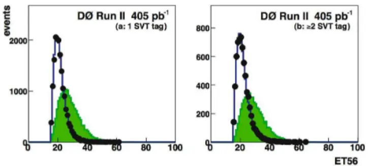
momenta of the jets (Fig. 1). (2) E56

T : The square root of the product of the

trans-verse momenta of the fifth and sixth leading jet (Fig. 2). (3) A: The aplanarity as calculated from the normal-ized momentum tensor (Fig. 3) [8, 9, 11].

FIG. 2: The E56

T distribution for single-tag events (a) and

double-tag events (b). Shown are the data (points), the back-ground (solid line) and the expected t¯t distribution (filled his-togram) multiplied by 140 (60) for the single (double)-tag analysis.

FIG. 3: The A distribution for single-tag events (a) and double-tag events (b). Shown are the data (points), the back-ground (solid line) and the expected t¯t distribution (filled his-togram) multiplied by 140 (60) for the single (double)-tag analysis.

(4) hη2

i: The pT-weighted mean square of the y of the

jets in an event (Fig. 4), see also Ref. [11].

(5) M: The mass-χ2 _{variable, which was defined as}

M = (MW1−MW) 2 /σ2 MW+(MW2−MW) 2 /σ2 MW+(mt1− mt₂)2/σm2t, where the parameters MW, σMW and σmt were the invariant mass and mass resolution from the jet

FIG. 4: The hη2

i distribution for single-tag events (a) and double-tag events (b). Shown are the data (points), the back-ground (solid line) and the expected t¯t distribution (filled his-togram) multiplied by 140 (60) for the single (double)-tag analysis.

FIG. 5: The M distribution for single-tag events (a) and double-tag events (b). Shown are the data (points), the back-ground (solid line) and the expected t¯t distribution (filled his-togram) multiplied by 140 (60) for the single (double)-tag analysis.

FIG. 6: The M34

mindistribution for single-tag events (a) and

double-tag events (b). Shown are the data (points), the back-ground (solid line) and the expected t¯t distribution (filled his-togram) multiplied by 140 (60) for the single (double)-tag analysis.

four-momenta calculated as observed in all-hadronic t¯t MC, respectively 79, 11 and 21 GeV/c2 _{after all}

correc-tions and resolucorrec-tions were included [12]. MWi and mti were calculated for every possible permutation of the jets in the event. We did not distinguish between tagged and untagged jets. The combination of jets that yielded the lowest value of M is used (Fig. 5).

(6) M34

min: The second-smallest dijet mass in the event.

First, all possible dijet masses were considered and the jets that yield the smallest mass were rejected. M34

min

was the smallest dijet mass as found from the remaining jets (Fig. 6).

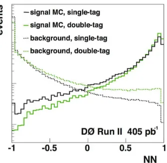
The top quark production cross section was calcu-lated from the output of NN, an artificial neural network trained to force its output near 1 for t¯t events and near −1 for QCD multijet events, using the multilayer perceptron in the root analysis program [13]. The six parameters illustrated in Figs. 1-6 were used as input for the neu-ral net. The very large background-to-signal ratio in the untagged data allowed us to use untagged data as back-ground input for the training of NN, while t¯t MC was used for the signal. Fig. 7 shows the NN discriminant for t¯t signal and multijet background. Although the distri-butions for single- and double-tag events were different

FIG. 7: The output discriminant of an artificial neural net-work (N N ) with six input nodes. All distributions are nor-malized to area. N N is optimized to distinguish between fully hadronic t¯t Monte Carlo events (signal) and the background from multijet production (background) as predicted by the tag rate functions.

due to increased heavy flavor content in the double-tag sample, both samples showed a clear discrimination be-tween signal and background.

The overwhelming background also made it possible to use the entire (tagged and untagged) sample to esti-mate the background. For the loose and tight SVT, we derived a tag rate function (trf — the probability for any individual jet to have a secondary vertex tag ) from the data with Ntags ≤ 1. The trf was parameterized

in terms of the pT, φ and y of the jet and the

coordi-nate along the beam axis (z) of the primary vertex of the event, zP V, in four different HT bins. To predict the

number of tagged jets in the event, it was necessary to correct for a possible correlation between tagged jets. In the single-tag analysis the correlation factor was negligi-ble, unlike in the double-tag analysis, where the presence of b¯b+jets events in the sample enhanced the correlation correction. We corrected for correlations caused by b¯b background by applying a correlation factor Cij, that

was parameterized as a function of the cone distance be-tween the tagged jets, ∆R. Figure 8 shows the number of double-tagged events versus ∆R as observed in data, and the distribution as modeled by the trf with and without including Cij. We considered significantly different

func-tional forms for the parameterization of Cij and found

that the choice of parameterization had little effect on the shape of the modeled background distribution.

The probabilities pi were used to assign a weight, the

FIG. 8: The performance of the trf prediction on double-tag events (points), without including the correlation factor Cij (dashed histogram), and including Cij for two different

functional parameterizations (solid histograms).

tags, to every tagged and untagged event in the sam-ple. To ensure the trf prediction was accurate in the region of phase space outside the “background” peak of the neural network, we used the region −0.7 < NN < 0.5 to determine a normalization. In this region of phase space, the t¯t content was negligible. A possible depen-dence on t¯t content was studied by the addition and/or subtraction of simulated t¯t events, as was the variation of the interval used for the normalization. Outside the background peak, the trf predictions were corrected by: SF_{1 = 1.000 ± 0.009 for the single-tag analysis, and} SF2 = 0.969 ± 0.014 for the double-tag analysis. The

errors on the normalization were taken into account as a systematic uncertainty on the number of background events.

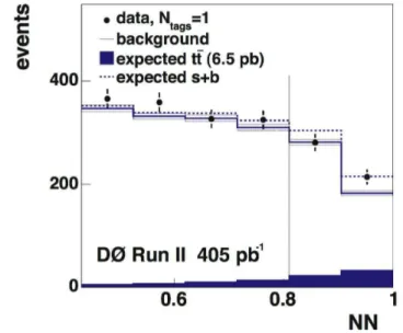
Both the single-tag and the double-tag analysis were expected to be dominated by background, even at large values of N N . Figures 9 and 10 show the distribution for data (points), the Monte Carlo simulation prediction for σt¯t= 6.5 pb (filled histogram), the background

pre-diction (line histogram) and the signal+background dis-tribution (dashed histogram) [9, 14].

The cross section was calculated from the number of t¯t and background candidates above a cut value of the N N discriminant. The cut value was chosen to maxi-mize the expected statistical significance s/√s + b, where s and b were the number of expected signal and back-ground events. The signal and backback-ground distributions were estimated using the trf prediction and t¯t Monte Carlo events [15]. For both analyses, the expected sta-tistical significance was about two standard deviations.

FIG. 9: The distribution of the N N output variable for single-tag events. Shown are the data (points), back-ground (hashed band), signal (filled histogram) and sig-nal+background (dashed histogram). The vertical line rep-resents the used cut of N N > 0.81.

The optimal cut for the single (double)-tag analysis was N N ≥ 0.81 (0.78) shown by a vertical line in Figs. 9 and 10. Table II gives the observed numbers of events (Ni

obs),

the background prediction (Ni

bg) and the efficiency for

signal (εt¯t) that can be used to calculate the t¯t

produc-tion cross secproduc-tion via:

σt¯t= Ni obs− Nbgi εi t¯tL(1 − ε i T RF) , (2)

where i was “= 1” for the single-tag analysis and “≥ 2” for the double-tag analysis. The number of background events is predicted using the trf method. It was likely that at values of N N close to unity a certain fraction of the sample used to predict the background actually consists of tagged or untagged t¯t events, resulting in an increased background prediction. The expected t¯t con-tamination of the background sample was corrected by a factor εi

T RF. In the higher value bins of N N , the

contri-bution from untagged t¯t events was significant. εi

T RF was

estimated by applying the trf on t¯t MC, and comparing the predicted tagging probability for signal to what was expected from background. The size of the Monte Carlo sample dominates the uncertainty on εi

T RF.

Table II lists the systematic uncertainties on the esti-mate of the number of background events, the selection efficiency and the background contamination. The first was uncorrelated between the two analyses, while the lat-ter two were correlated as they were derived from the same Monte Carlo samples.

TABLE II: Overview of observed events, background predic-tions and efficiencies.

symbol value observed events N=1 obs 495 background events N=1 bg 464.3 ± 4.6(syst) t¯t efficiency ε=1 t¯t 0.0242 +0.0049 −0.0058(syst) t¯t contamination ε=1 T RF 0.245 ± 0.031(syst) observed events N≥2 obs 439 background events Nbg≥2 400.2 +7.3 −6.2(syst) t¯t efficiency ε≥2_t¯t 0.0254+0.0065 −0.0070(syst) t¯t contamination ε≥2 T RF 0.194 ± 0.048(syst)

FIG. 10: The distribution of the N N output variable for double-tag events. Shown are the data (points), back-ground (hashed band), signal (filled histogram) and sig-nal+background (dashed histogram). The vertical line rep-resents the used cut of N N > 0.78.

on the selection efficiency was dominated by the uncer-tainty in the jet calibration and identification, which were estimated by varying the parameterizations used by one standard deviation. The uncertainty on the background prediction was dominated by the uncertainty on the trf method and the uncertainty on εT RF was due to

lim-ited Monte Carlo statistics. The uncertainty of the trf prediction was comprised from the uncertainties coming from the fits of the probability density functions at the jet level, the statistics of the background sample and the

uncertainty on the normalization and correlation factors SF and Cij. For the double-tag analysis, the

contribu-tion from the uncertainties due to calibracontribu-tion of the b quark jet identification efficiency was an additional sys-tematic uncertainty on εt¯t. These uncertainties were

de-rived by varying the parameterizations used within their known uncertainties.

The single-tag analysis yielded a cross section of

σt¯t= 4.1+3.0−3.0(stat) +1.3

−0.9(syst) ± 0.3(lumi) pb. (3)

For the double-tag analysis the measured cross section was

σt¯t= 4.7+2.6_−2.5(stat)+1.7_−1.4(syst) ± 0.3(lumi) pb. (4)

As the single-tag and double-tag analysis were mea-sured on independent samples, the statistical uncertain-ties were uncorrelated. The uncertainuncertain-ties on the selection efficiency were completely correlated. Taking all uncer-tainties into account, a combined cross section measure-ment of

σt¯t= 4.5+2.0−1.9(stat) +1.4

−1.1(syst) ± 0.3(lumi) pb (5)

was obtained, for a top quark mass of mt= 175 GeV/c2.

For a top quark mass of mt = 165 GeV/c2, the cross

section is σt¯t(165) = 6.2+2.8−2.7(stat) +2.0

−1.5(syst) ± 0.4(lumi)

pb, while for a top quark mass of mt= 185 GeV/c2the

value shifted down to σt¯t(185) = 4.3+1.9−1.8(stat) +1.4 −1.0(syst)±

0.3(lumi) pb.

In summary, we have measured the t¯t production cross section in p¯p interactions at√s = 1.96 TeV in the fully hadronic decay channel. We used lifetime b-tagging and an artificial neural network to distinguish t¯t from back-ground. Our measurement yields a value consistent with SM predictions and previous measurements.

We thank the staffs at Fermilab and collaborating in-stitutions, and acknowledge support from the DOE and NSF (USA); CEA and CNRS/IN2P3 (France); FASI, Rosatom and RFBR (Russia); CAPES, CNPq, FAPERJ, FAPESP and FUNDUNESP (Brazil); DAE and DST (India); Colciencias (Colombia); CONACyT (Mexico); KRF and KOSEF (Korea); CONICET and UBACyT (Argentina); FOM (The Netherlands); PPARC (United Kingdom); MSMT (Czech Republic); CRC Program, CFI, NSERC and WestGrid Project (Canada); BMBF and DFG (Germany); SFI (Ireland); The Swedish Re-search Council (Sweden); ReRe-search Corporation; Alexan-der von Humboldt Foundation; and the Marie Curie Pro-gram.

[*] Visitor from Augustana College, Sioux Falls, SD, USA [†] Visitor from Helsinki Institute of Physics, Helsinki,

Fin-land.

[1] DØ Collaboration, V.M. Abazov et al., Nucl. Instrum.

Methods Phys. Res. A 565, 463 (2006).

[2] T. Andeen et. al., FERMILAB-TM-2365-E (2006), in preparation.

throughout the data collection period. Efficiencies were was measured both on t¯t Monte Carlo and derived from parameterizations determined from data.

[4] M.L. Mangano et al., J. High Energy Phys. 07, 001 (2003).

[5] T. Sj¨ostrand et al., Comput. Phys. Commun. 135, 238 (2001).

[6] D. Lange, Nucl. Instrum. Methods Phys. Res. A 462, 152 (2001).

[7] G.C. Blazey et al., in Proceedings of the Workshop: QCD

and Weak Boson Physics in Run II, U. Baur, R.K. Ellis and D. Zeppenfeld (ed.), Fermilab, Batavia, IL (2000). [8] DØ Collaboration, V.M. Abazov et al., Phys. Lett. B

626_{, 35 (2005).}

[9] DØ Collaboration, V.M. Abazov et al., Submitted to Phys. Rev. D, FERMILAB-PUB-06-386-E (2006).

[10] W.-M. Yao et al., Journal of Physics G 33, 1 (2006). [11] DØ Collaboration, B. Abbott et al., Phys. Rev. Lett. 83

1908 (1999).

[12] The possibility that the wrong permutations of jets could be chosen was taken into account in the determination of the values of the values of 79, 11, and 21 GeV/c2_{for M}

W,

σM_W and σmt.

[13] R. Brun and F. Rademakers, Nucl. Inst. Meth. in Phys. Res. A 389 (1997) 81-86. See also http://root.cern.ch/. [14] N. Kidonakis and R. Vogt, Phys. Rev. D 68, 114014

(2003).

[15] The expected t¯t content used to optimize the N N cut was equivalent with a hypothetical cross section of σt¯t=

6.5 pb. The chosen cuts are stable under variation of the value assumed for the optimization.