Flow-field analysis of anti-kidney vortex film cooling

(1)

This work was partly funded by Swiss National Science Foundation (SNF) with project number 200020-116310. Received: October 2011

Lars Gräf: Doctoral candidate

www.springerlink.com DOI: 10.1007/s11630-012-0520-y Article ID: 1003-2169(2012)01-0066-11

Flow-Field Analysis of Anti-Kidney Vortex Film Cooling

Lars Gräf and Leonhard Kleiser

Institute of Fluid Dynamics, ETH Zurich, 8092 Zürich, Switzerland

Film cooling is an important measure to enable an increase of the inlet temperature of a gas turbine and, thereby, to improve its overall efficiency. The coolant is ejected through spanwise rows of holes in the blades or endwalls to build up a film shielding the material. The holes often are inclined in the downstream direction and give rise to a kidney vortex. This is a counter-rotating vortex pair, with an upward flow direction between the two vortices, which tends to lift off the surface and to locally feed hot air towards the blade outside the pair. Reversing the rota-tional sense of the vortices reverses these two drawbacks into advantages. In the considered case, an anti-kidney vortex is generated using two subsequent rows of holes both inclined downstream and yawed spanwise with al-ternating angles. In a previous study, we performed large-eddy simulations (which focused on the fully turbulent boundary layer) of this anti-kidney vortex film-cooling and compared them to a corresponding physical experi-ment. The present work analyzes the simulated flow field in detail, beginning in the plenum (inside the blade or endwall) through the holes up to the mixture with the hot boundary layer. To identify the vortical structures found in the mean flow and in the instantaneous flow, we mostly use the λ2 criterion and the line integral convolution (LIC) technique indicating sectional streamlines. The flow regions (coolant plenum, holes, and boundary layer) are studied subsequently and linked to each other. To track the anti-kidney vortex throughout the boundary layer, we propose two criteria which are based on vorticity and on LIC results. This enables us to associate the jet vor-tices with the cooling effectiveness at the wall, which is the key feature of film cooling.

Keywords: Film cooling, anti-kidney vortex, vortex identification, trajectory tracking, large-eddy simulation, LES,compound angle, double row, kidney vortex, jet in cross-flow.

Introduction

Film cooling is one measure which allows for a higher turbine inlet temperature and, hence, an increased gas turbine efficiency. Usually, spanwise rows of holes (di-ameter d) are drilled into the surface to be cooled. These holes (pipes) duct the cold fluid from the interior (ple-num) to establish a coolant film shielding the wall mate-rial from the approaching hot gas (Fig. 1.a). For a further explanation see [1].

The discrete holes which are commonly inclined by a simple angle 0° ≤ α ≤ 90° (Fig. 1.b, β = 0°) establish a kidney vortex by the interaction with the cross-flow (ve-locity U∞), e.g. [2–4]. This counter-rotating vortex pair changes the cooling effectiveness to the worse for two reasons. First, it feeds hot gas towards the surface outside of the vortex-pair. Second, the mutually induced velocities from the individual vortices point away from the sur-face to be cooled. This favors the lift-off of the coolant jet. There are three basic approaches to improve the cool-

(2)

Nomenclature

d hole diameter Subscripts

p pressure 1 upstream pipe

t time 2 downstream pipe

u, v, w velocity components in spatial directions 5 %, 95 % iso-value of 0.05, 0.95

U∞ cross-flow velocity Operators and Notation

x, y, z downstream, wall-normal, spanwise coordinate <>t averaging of  over t

Greek letters x vector (lower case)

 inclination angle S tensor (upper case)

 yaw angle Abbreviations

 boundary layer thickness bl boundary layer

‘,  coordinates cw clockwise

 adiabatic film cooling effectiveness ccw counter-clockwise

 momentum thickness LES Large-Eddy Simulation

λ vortex criterion LIC line integral convolution

 scalar pi pipe(s)

 vorticity pl plenum

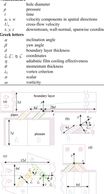
Fig. 1 Computational domain and coordinate systems. (a):

side view; (b): swept side view; (c): top view; (d): downstream view. Solid thick: visible edge; dashed: invisible edge; dash-dotted: centerline; hatched: wall; blue: coolant; red: hot gas.

ing effectiveness. They might be combined but their beneficial effect does not add up necessarily. First, yawing the hole additionally in the spanwise direction by an angle β ≠ 0°, referred to as compound angle (Fig. 1.c), results in one principal vortex [5]. This improves the cooling effectiveness at the price of a higher heat transfer coefficient. Second, Ref. [6] concluded that a hole that is wider in the spanwise than in the streamwise direction, as in the so-called shaped hole exit, gives rise to an

addi-tional vortex pair, termed anti-kidney vortex. It exhibits a reversed rotational direction compared to a kidney vortex. The anti-kidney vortex modifies the dominant kidney vortex formed at the lateral edges of the hole. In addition, Ref. [6] reported a reduced tendency of the jet to lift-off in cases where there is an anti-kidney vortex present. Finally, the interaction of multiple, closely-spaced holes is beneficial to the cooling effectiveness.Either multiple rows, arranged from in-line to staggered [7], or arrays of holes are employed [8–10]. The interaction of the holes modifies the dominant vortices or improves the spanwise coverage of the coolant.

Anti-kidney vortices do not exhibit the detrimental features of kidney vortices. In [11, 12], two subsequent rows of compound-angle holes generate the two vortices which together yield an anti-kidney vortex. The opposite rotational sense of the vortices is obtained by a positive compound angle of the upstream row and a negative compound angle of the downstream row (Fig. 1.c).A reference experiment [11] shows that this arrangement provides a higher cooling effectiveness than a sim-ple-angle coolant ejection. Reference [11] did not present results on the flow inside the plenum or in the pipes. In addition, they did not show data which explains the vor-tex pair's subsequent assembling by the individual rows.

In previous work [13], we have shown that results of our Large-Eddy simulations (LES) compare well with the reference experiment. Reference [13] also gives a more detailed review on existing simulation results of film cooling. The present paper focuses on a detailed analysis of the anti-kidney vortex film-cooling results of [13, case 3] (α = 35°, |β| = 45°) in plenum, pipes, and boundary layer.

Subsection Methods, Simulation briefly presents the modeling approach, followed by the methods used for visualization in Subsec. Methods, Visualization. Starting

(3)

from the plenum over the pipes to the boundary layer and film, the mean primary and secondary flow is subse-quently studied in detail. Then, the instantaneous flow field is discussed and the last section draws conclusions of the present paper.

Methods Simulation

As in the earlier paper [13], we performed numerical computations of the Navier-Stokes equations to simulate the film cooling flow-field, using the structured, multi-block, finite-volume code NSMB [14]. Computa-tional aspects of the setup used are discussed in [15]. The advection and diffusion terms are discretized by centered fourth- and second-order accurate schemes, respectively; a second-order Runge-Kutta scheme is employed to ad-vance the solution in time. LES of the flow are per-formed to save computational resources. The relaxation term of the approximate deconvolution model [16, RT-3D] accounts for the non-resolved scales.

The inflow into the boundary layer is time-dependent and turbulent. It is defined by the synthetic-eddy method [17] modified for use in the compressible regime [18]. In contrast, the plenum inflow is considered laminar and chosen as a steady, plane Poiseuille velocity profile. The ambient and outflow zones are modeled by non-reflect- ing characteristic boundary conditions [19]. Sponges located at x/d ≤ 9, x/d ≥ 25, y/d ≲ 7.3, and y/d > 4 supplement the steady in- and outflow conditions.The walls are considered adiabatic and spanwise periodicity (Fig. 3.a) models infinitely long rows of coolant holes. Visualization

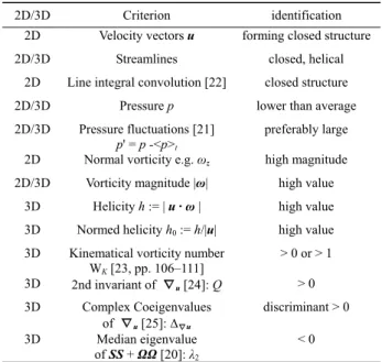
Vortex structures play an important role for this spe-cific film-cooling arrangement (Sec. Introduction). The existence of various criteria displayed in Table 1 reflects the ambiguous definition of a vortex [20, 21].

The line integral convolution (LIC) method [22] is chosen to visualize the velocity components perpendicu-lar to the vortex axis. Two shortcomings of LIC are that it neither reveals information on the magnitude (vortex strength) nor on the rotational sense of the vortex. In contrast to the normal vorticity, LIC fails to predict the correct position of the vortex core if the vortex axis is not cut perpendicularly. Therefore, such gray-scale images often colored by the axial vorticity and velocity vectors are depicted next to the LIC (Figs. 5, 7). Furthermore, experience with the LES results revealed that a tilted vortex can appear as twins of small, co-rotating vortices (Figs. 5.g,h).

To convey an impression of the three-dimensional shape of a vortex, the λ2 criterion [20] is employed.

Strictly speaking, every negative λ2 value identifies a

Table 1 Vortex identification criteria. Principally ordered by

decreasing intuitiveness and increasing elaborateness. S, Ω: symmetric and anti-symmetric part of ∇u, respectively.

2D/3D Criterion identification 2D Velocity vectors u forming closed structure

2D/3D Streamlines closed, helical 2D Line integral convolution [22] closed structure

2D/3D Pressure p lower than average 2D/3D Pressure fluctuations [21]

p' = p -<p>t

preferably large 2D Normal vorticity e.g. ωz high magnitude

2D/3D Vorticity magnitude |ω| high value 3D Helicity h := | u · ω | high value 3D Normed helicity h0 := h/|u| high value

3D Kinematical vorticity number WK [23, pp. 106–111] > 0 or > 1 3D 2nd invariant of ∇u [24]: Q > 0 3D Complex Coeigenvalues of ∇u [25]: ∆∇u discriminant > 0 3D Median eigenvalue of SS + ΩΩ [20]: λ2 < 0

vortex. Usually it is assumed that smaller λ2 values

rep-resent stronger vortices, although there is no theoretical justification. Consequently, we often present iso-surfaces of λ2 values smaller than zero to filter only the important

vortical structures. As customary, isobars of low pressure levels are used to emphasize yet stronger vortices.

Plenum

A number of right-handed Cartesian coordinate systems are introduced (Fig. 1) to keep track of the position of the various views and cross-sections. The principal system (x,

y, z) has its origin at the downstream pipe (index: 2). By

first translating it to the upstream pipe (index: 1) and then yawing around the y-axis by the compound angle β, an additional system (ξ1, y, ζ1) is obtained. Another rotation

by 90° - α around ζ1 yields the coordinate system (ξ'1, η1,

ζ1) that is aligned with the pipe axis (depending on the

context, η also denotes the cooling effectiveness). Like-wise, the systems (ξ2, y, ζ2) and (ξ'2, η2, ζ2) are intro

duced; they share their origin with (x, y, z). For later ref-erence, a table of vortices (Table 2) identifies the various vortices that will appear throughout the paper.

The simulation of the coolant flow started with a fic-tive channel flow in the y-direction (see velocity vectors at the bottom of Fig. 2.a). Inside a real turbine blade, the coolant supply-flow in general follows the ±z-direction superimposed by rotational effects which deflect the flow mainly in the other blade-parallel direction (±x). How-ever as the flow approaches the pipes, it is oriented to-wards the blade surface (y-direction). At this point, the presented simulation begins.

(4)

Table 2 Table of vortices. Number (No.); sense of rotation in viewing direction (dir.): clockwise (cw) or counter-clockwise (ccw).

No. dir. association note cf. Sec. or Subsec. {1} ccw upstream pipe corner Plenum, Secondary Flow Field

{2} cw downstream pipe corner Plenum, Secondary Flow Field

{3} n/a plenum, both pipes torus Plenum, Secondary Flow Field

{4} cw both pipes separation Pipes, Primary Flow Field

{5} cw upstream pipe principal Pipes, Secondary Flow Field; Boundary Layer

{6} ccw downstream pipe principal Pipes, Secondary Flow Field; Boundary Layer

{7} ccw upstream pipe degenerated Pipes, Secondary Flow Field; Boundary Layer, Secondary Flow Field {8} cw downstream pipe degenerated Pipes, Secondary Flow Field; Boundary Layer, Secondary Flow Field {9} cw upstream pipe secondary Pipes, Secondary Flow Field; Boundary Layer, Secondary Flow Field {10} ccw downstream pipe secondary Pipes, Secondary Flow Field; Boundary Layer, Secondary Flow Field {11} ccw upstream pipe secondary Pipes, Secondary Flow Field; Boundary Layer, Secondary Flow Field {12} cw downstream pipe secondary Pipes, Secondary Flow Field; Boundary Layer, Secondary Flow Field {13} cw upstream pipe horseshoe Boundary Layer, Secondary Flow Field

{14} ccw downstream pipe horseshoe Boundary Layer, Secondary Flow Field

{15} n/a both pipes streak Instantaneous Flow Field

{16} n/a both pipes roll up Instantaneous Flow Field

Mean Primary Flow

The primary flow in the plenum is characterized by the sudden contraction of a wide channel to a narrow pipe flow. In general, the field is oriented in the y-direc-tion and accelerated while approaching the plenum–pipe orifice (Fig. 2). As expected intuitively, the flow is dis-tributed in a regular fashion among the individual pipes (Fig. 2.b).

Mean SecondaryFlow

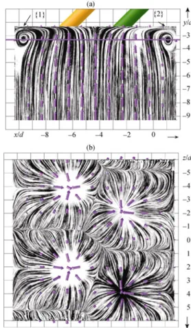
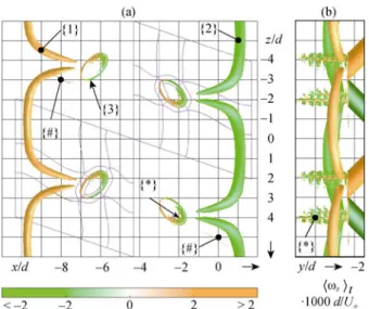
The secondary flow reveals two different systems of structures: the corner {1,2} and the torus {3} vortices. (There are also some numerical artefacts such as the crescent {*} and the block-edge {#} structures.) In most channel contractions, a pair of counter-rotating corner vortices appears [26, Fig. 7.10]. For the present case, these vortices are identified as {1,2} and revolve slowly (Figs. 2.a, 3). These corner vortices are sucked in towards the nearest pipe (Fig. 3.a) following the principal flow. The velocity vectors in Fig. 2.b show the acceleration of the primary flow which transports the corner vortex to-wards the plenum–pipe orifice where it breaks up. A link to the counter-rotating vortex pair {5,6} cannot be made due to the large spatial distance. The downstream view in Fig. 3.b shows that the corner vortex near the down-stream pipe occupies more space than the other one. This asymmetry can be explained by the inclination of the pipes. The acute angle of the downstream pipe causes the flow to detach earlier from the plenum wall at x/d ≈ 1.7, thus increasing the space available for the corner vortex.

At the plenum–pipe orifices, relatively thin to-rus-shaped structures {3} establish themselves. The

ma-jor part of them is located within the pipe.They are also reported for a simple-angle film cooling flow in [27].

Fig. 2 Mean primary flow in the plenum. Cross-sections at (a):

z/d = 0; (b): y/d ≈ -3.3 (through the corner vortex cores). Gray-scale: LIC; purple vector: velocity; purple line: position of cross-section.

(5)

Fig. 3 Corner vortices. (a): Top view; (b): front view on <λ2>t

= 2×104_{surfaces colored by the spanwise vorticity} <ωz >t d/U∞ of the plenum (y/d 2.3). Purple: block grid.

These rings partly block the view on the crescent arte-facts {*} located at the acute-angled section of the orifice ellipses. Together with the thin structures {#} (Fig. 3), we consider them numerical artefacts. They are either caused by locally insufficient resolution or smoothness of the computational grid. The small |λ2|level at which the

ar-tefacts become visible suggests a small effect on the flow field.

Pipes

Following the coolant flow, we study the upstream pipe and subsequently highlight the differences to the downstream pipe.

As expected downstream a sharp-edged inlet [26, Fig. 7.10], a contraction of the streamlines is observed (Fig. 4.c) with its maximum around η1/d = 3.75. One might

expect the largest axial velocity at the same location. This is not the case, however, (see also Figs. 5.d,e) because the pipe is not yet closed in circumferential direction (Fig. 4.a).In addition, the flow is asymmetric (Fig. 4.c) which is attributed to the compound angle. Downstream of η1/d

≈ – 1.5, the flow is oriented in the ζ1-direction which is a

consequence of the strong cross-flow momentum in the

x-direction.

In another axial cross-section (Fig. 4.a), a large sepa-ration bubble {4} with a recirculation zone is visible downstream of the acute-angled edge (positive ξ'1). At the

opposing wall (negative ξ'1), commonly referred to as

jetting region, the axial velocity is maximal. The flow asymmetry is caused by the inclination of the pipe and

Fig. 4 Mean primary flow in the pipes. LIC of (a), (b):

<uξ'1,2,uη1,2>t/U∞; (c), (d): <uζ1,2,uη1,2>t/U∞ colored by axial velocity <uη1,2>t/U∞ in cross-sections at (a), (b): ζ1,2/d = 0; (c), (d): ξ’1,2/d = 0. (a), (c): upstream; (b), (d): downstream pipe. Purple line: positions of cross- section in Fig. 5.

the inertia of the fluid. Thequalitative behavior in the downstream pipe is the same (Figs. 4.b,d, 5.t). Consis-tently, the flow is bend towards the - ζ2-direction due to

the opposite compound-angle.

Deeper insight into the flow is gained from studying radial–circumferential cross-sections as depicted in Fig. 5. Surprisingly, the separation bubble is not located at the acute-angled boundary (ξ'1/d = 0.5) but is revolved

coun-ter-clockwise by roughly 30° towards positive ζ1 (Fig.

5.d). This revolved state continues as we move upstream (Figs. 5.c,b) and is addressed in Subsec. Pipes, Mean Secondary Flow. Nevertheless, the axial velocity-field is approximately symmetric to ζ1/d = 0 close to the coolant

ejection and is revolved clockwise (Fig. 5.a). The latter revolution is caused most probably by the strong cross-flow momentum in the x-direction.

The flow in the downstream pipe shows the same re-volved tendency, surprisingly also towards the coun-ter-clockwise direction (Figs. 5.q–s).As expected, the downstream cross-sections of the pipes exhibit mir-ror-symmetric tendencies (Figs. 5.a,p) due to the opposite compound-angle β.

(6)

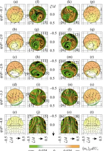
Fig. 5 Time-averaged development of the velocity field along

the pipe axis.(a)–(e), (p)–(t): iso-contours of the axial velocity <uη1,2>t/U∞ (iso-levels at - 0.5, 0.0 … 2.0, colorbar in Fig. 4) and vectors of normal velocities <uξ'1,2,uζ1,2>t/U∞ (row-specific reference at the outer side equals 0.4 U∞); (f)–(o): LIC of normal velocities colored by axial vorticity <ωη1,2>t d/U∞.(a)–(j): up-stream pipe; (k)–(t): downup-stream pipe.

in the secondary flow in the upstream pipe.They are dri-ven by the entering pipe flow and, consequently, show opposite sense of rotation. Following the flow in the pipe, a system of four vortices develops, which exhibits alter-nating rotational directions (Figs. 5.i–g). This is also ob-served in [27, Fig. 9.d].The second counter-clockwise rotating vortex {9} (appearing as twins in Figs. 5.g,h, see Subsec. Methods, Visualization) is stronger than its counter-part {11}. The second vortex pair {9,11} might establish itself due to the deflection of the turbulent flow as in a 90° pipe elbow [26, Fig. 7.14]. The counter- clockwise rotating vortex of the initial pair is linked to the principal vortex of the upstream hole, due to its spa-tial position and rotational sense (Figs. 8.b, 7.f). In addi-tion, the origin of the kidney vortex at the pipe–plenum orifice is shown in [27] for a simple-angle ejection case.

The revolved flow-field, described in Subsec. Pipes, Mean Primary Flow, is visible more clearly in Figs.

5.f–j. Moreover, the LIC images suggest that the initial negative u1 velocity component near '1/d = - 0.5 cause

the overall counter-clockwise revolution of the flow (Fig. 5.j). However, we could not yet find a reason for the negative velocity component.

In the downstream pipe, the secondary flow is similar up to 2/d = 2 (Figs. 5. o–m, j–h). At 2/d = - 0.7, the

counter-clockwise vortex is the most intense (Fig. 5.k). A reason for this, perhaps counter-intuitive, behavior is given in Subsec. Pipes, Mean Primary Flow.

Boundary Layer and Cooling Film

A preliminary and brief explanation of the bound-ary-layer (or film) area is given in [13, Sec. 4.5, Fig. 11] and [15, Sec. 3.3, Fig. 8] based on streamline visualiza-tions.To extend these considerations, we first analyze the mean primary flow field.

The spanwise-averaged velocity thickness δU,95% (de-fined in the caption of Fig. 6) is one characteristic meas-ure of a boundary layer. The non-monotonic behavior of the thickness upstream of x/d ≈ 10 (Fig. 6.a) clearly is a consequence of the strongly, three-dimensionally dis-turbed flow. Farther downstream, the thickening of the film-cooled boundary layer, also reported in [28], appears to be steady and the thickening was more intense com-pared to a canonical boundary layer [13, case 2].

Besides the thickness, the trajectories of the coolant jets are interesting to be tracked. Reference [29] identi-fied the trajectories of a generic jet-in-crossflow by dif-ferent measures: streamlines, velocity maximum, and scalar-concentration maximum. For the latter two, the location of the maxima in yz-planes was monitored. First, from the streamlines [13, Fig. 11; 15, Fig. 8] it is hard to choose a representative line which characterizes the path of one coolant jet. Second, the maximum velocity crite-rion cannot distinguish the two jets. Since the two jets stem from the same plenum, the concentration criterion also fails.

Moving on to identify the jet trajectories, the vortices come into play. As introduced in Sec. Introduction, the cooling profits from the presence of an anti-kidney vor-tex. Therefore, the vortex trajectories are supposed to be congruent with thetrajectories. The question arises how the vortices can be identified throughout the domain. In the preceding sections, the vortex identification is done using LIC, vorticity, and λ2 criteria. Figure 8 shows that

iso-surfaces of λ2 quickly loose track of the vortex as it

diffuses downstream.

Determining a maximum λ2 curve in the sense of [29]

does not help to distinguish the jets.However, a charac-teristic feature is the rotational sense, which can be iden-

(7)

Fig. 6 Downstream development of the mean flow. (a): spanwise averaged boundary layer thicknesses; ( , ): velocity δU∞,95%: <u>z,t/U∞ = 0.95; ( ): with coolant ejection (present case); ( ): without ejection [13, case 2]; ( ): temperature δθ,5%: <θ>z,t = 0.05. (b), (c): ( , ): smoothed coolant-jet trajectories of the upstream ( , ) and

the downstream pipe ( , ); ( ): LIC trajectory; ( ): vorticity trajectory; ( ): pipe; ( ): iso-lines (levels 0.25, 0.30 … 0.50) of film cooling effectiveness <η>t [13, Fig. 14.a].

tified by the downstream vorticity ωx. Since the peak of positive or negative ωx is not necessarily located in the vortex core and there were some smaller vortices around, the field is integrated following





int( ) 1₂ clip( ) d ' d ' , , , , ' [0, ', '] , σ x, x, σ ω ω ' y z σ x y z y z     

 

x x x x x

using σ/d = 0.4. Between each principal vortex {5,6} and the wall, an area of strong opposite vorticity is present (Figs. 7.a,b,f). There, the vorticity ωx is very strong and exhibits the opposite sign due to the no-slip boundary condition. To clip this zone, the vorticity ωx,clip is set to zero below the arbitrarily chosen threshold yclip/d = 0.2.

As a second criterion, the centers of the vortex-pair visualized using LIC (Figs. 7.a–f) are determined manu-ally. In the vicinity of the downstream ejection, the LIC does not show a circular structure for vortex {5} (Figs. 7.d,e). Most probably, the reason is that the cross-section does not cut the vortex axis perpendicularly. In this case, the center is estimated to be at the strongest curved structure exhibiting the expected vorticity.

Figures 6.b,c compare the results of the above men-tioned criteria to identify the vortex trajectories. The projection in the - y-direction (Fig. 6.c) shows larger dif-ferences only for the upstream-jet trajectories {5} in the vicinity of the downstream ejection, which might be due to the ambiguous results of the vortex core identified by LIC (Figs. 7.d,e).The projection in the - z-direction (Fig. 6.b) reveals that the vorticity criterion results in a trajec-

tory closer to the wall compared to the LIC criterion. Especially for x/d > 15, the wall-distance of the vorticity criterion is the same for both jets, whereas LIC identifies the vortex core of the upstream jet {5} farther away from the wall. Figure 7.a. shows that both vortices have a wall-normal elongated shape above their cores. Below the cores, this results in stronger velocity gradients and thus vorticities.The elongation of the clockwise vortex is more intense which results in a bigger disagreement be-tween the criteria.

Interestingly, the upstream vortex {5} penetrates into the free-stream area, as identified by δU∞,95%, only for a short distance downstream of the coolant ejection (Fig. 6.b). The downstream vortex {6} never leaves the boundary layer and downstream of x/d = 18 both {5,6} are parallel to the wall.

The spanwise-averaged coolant film, identified by δθ, 5% starts right at the upstream edge of the upstream ejection. After a small separation bubble downstream of x/d ≈ 0.7, it slightly overshoots δU, 95% to swing back and to follow the velocity thickness in parallel for x/d > 20.

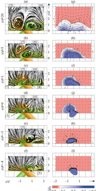
Following the boundary-layer flow, the approaching hot gas is slightly displaced from the wall (δU,95% in Fig. 6.a) by the partial blockage of the upstream coolant row. Then, coolant is ejected in the -z-direction (Fig. 7.l) gen-erating a clockwise vortex {5} at the leeward edge of the orifice (Figs. 7.f,e). This vortex transports hot cross-flow fluid towards the plate. Thereby, it sucks in hot fluid and transports it in helical paths [13, Fig. 11], [15, Fig. 8]. The spanwise trajectory (Figs. 6.c, 8.b) is tilted by 20°

(8)

Fig. 7 Time-averaged development of the normal velocities

<v,w>t/U∞ and the temperature <θ>t. (a)–(f): LIC

col-ored by the downstream vorticity <ωx>t d/U∞ (colorbar in Fig. 5); (g)–(l): iso-contours (at levels 0.05, 0.10 … 0.50) of the temperature with velocity vectors (the section-specific reference at outer side equals 0.15 U∞).

25° in the direction of the compound angle β due to the resulting momentum between the jet and the cross-flow. Shortly upstream the downstream ejection, the vortex is initially displaced from the wall, similar to the cross-flow at the upstream pipe. The blockage effect of the down-stream coolant widens the clockwise vortex in the span-wise direction (Figs. 7.d,c,j).

The downstream jet faces this disturbed flow field. The resulting momentum causes the counter-clockwise vortex {6} to be tilted by roughly -10° with respect to the cross-flow (Figs. 6.c, 8.b). The magnitude of the

Fig. 8 Time-averaged iso-surfaces of <λ2>t = - 0.5 colored by

downstream vorticity <ωx>t d/U∞ (colorbar see Fig. 3). (a): side view; (b): top view. Purple line: positions of cross-sections in Fig. 7.

deflection of the downstream vortex is smaller due to the already positively tilted disturbed flow.

Farther downstream, the counter-clockwise vortex {5} is revolved around the clockwise vortex {6} due to the induced velocity of the latter (Figs. 7.d–b). Finally, they come to rest side by side (Fig. 7.a) still exhibiting a slightly asymmetric spanwise and wall-normal coverage, as already observed in [13, 15].

Considering the coolant distribution normal to the cross-flow, Figs. 7.k,i,h show that the temperature gradi-ent flattens with increasing distance to the ejection. This generates a strongly asymmetric distribution in Fig. 7.i. The reference velocity in Figs. 7.i–g shows the weaken-ing of the vortices with the downstream coordinate x. As intended, the spanwise growth of the film is more pro-nounced than the wall-normal one (Figs. 7.i–g). This is attributed to the rotational sense of the anti-kidney vortex. Close to the wall, cold fluid from the pair-interior is driven outside.This is confirmed by Fig. 6.c showing cooling peaks mostly outside of the cores. Away from the wall, however, the vortex pair entrains hot fluid which creates a local minimum of cooling beneath the common vortex-core.

Coming to the mean secondary flow, Figs. 8.b, 7f–d identify more than the principal vortex pair {5,6}. First, one leg of the degenerated horseshoe-vortex at each hole {13,14} is visible. As one moves around the upstream hole, four vortices with alternating rotational direction are distinguishable. The symmetric picture (spanwise broadened) is obvious at the downstream hole. All four vortices are clearly visible in Fig. 8.b, and some can also be suspected in Figs. 7e–c, marked by their numbers.

The two small vortices (the outer one is suspected to be the degenerated one, since it is the strongest among the three weak ones) with the same direction merges into

(9)

Fig. 9 Instantaneous flow. Iso-surfaces of λ2 = 1.5 colored by temperature θ (colorbar in Fig. 7 using black instead of white). (a): bottom view; (b): side view; (c): top view. Zones showing no instantaneous activity (|y|/d > 3) and sponges are clipped. one while the remaining third small structure quickly

diffuses. This scenario is more obvious for the upstream pipe and, probably, develops in a more elongated manner at the downstream hole.While the principal vortices de-tach from the wall, the degenerated one remains atde-tached as observed also in experiments of single-row com-pound-angle cooling [30].

Instantaneous Flow

Figure 9 depicts instantaneous vortical structures. Starting just downstream of the inflow sponge, the bot-tom view shows streaky structures, whereas the side view reveals hairpin-like vortices (Figs. 9.a,b). Both are char-acteristic for turbulent boundary layers [31].The bound-ary-layer vortices seem to pile up on the - z-side up-stream of the upup-stream pipe due to the partial blockage by the coolant (Fig. 9.c). On the other side, they are transported underneath the coolant jet (Fig. 9.a).

Figure 10 shows the stronger and strongest vortices identified by the λ2 criterion and by pressure iso-surfaces,

respectively, emphasizing the vortices in the area of the coolant ejection. Just upstream of the plenum–pipe ori-fices, the weak crescent artefacts {*} and torus {3} vor-tices emerge (Fig. 9.b, Subsec. Plenum, Mean Secon-dary Flow). Downstream of the orifice, the separation bubble appears as a zone of depression. Further on, strong (Fig. 10.b) and weak (Figs. 9.a,b) streaky struc-tures {15} develop and break up near and downstream of the pipe-boundary-layer orifice. At the origin of the shear-layer between approaching flow and coolant, roll-ups {16}, which are characteristic to jet-in-crossflow

scenarios [3, 4]. The roll-ups follow the shear-layer being attached to the principal vortex at one side and getting weaker at the other. Downstream roughly 1.5 d, they de-tach from the principal vortex and diffuse (Fig. 10.b). Repetitious accumulations{16},which are probably a

Fig. 10 Instantaneous flow in the vicinity of the coolant

ejec-tion posiejec-tions. Brown: iso-surfaces of λ2 = 30; green: of p/p∞ = 0.9828. (a): top view; (b): oblique view. Opaque Purple: pipes and plate.

(10)

result of the roll-ups, can be suspected in Fig. 9.c. How-ever, hairpin vortices stemming from the detaching legs of the horseshoe vortex [27, Sec. 3.1] are not found.A reason for that may be the lacking second leg of the horseshoe. The vortical structures in the vicinity of the two pipe–boundary-layer orifices are similar although they showed distinct peculiarities due to a different effec-tive approaching flow.

The wall-normal region filled with vortical structures thickens considerably due to the coolant ejections up to

x/d ≈ 5 (Fig. 9.b). Downstream of x/d ≈ 10, the coolant

vortices become more streaky due to weaker principal vortices.In the same region, the vortical structures show gaps (x/d ≈ 13, 21) and accumulations (x/d ≈ 16) which may be a result of the roll-up merging into bigger, less intense spanwise packages which travel downstream. Moreover, the package heights indicate an increasing thickness of the boundary layer.

Conclusions

In the present paper, we presented a detailed analysis of an anti-kidney vortex film-cooling flow obtained by LES. The computational domain includes the plenum, the pipes, and the boundary layer. We demonstrate the mu-tual connection of the various flow phenomena in these regions.

In the (design-specific) edges of the plenum, we ob-serve slowly revolving vortices which are sucked to-wards the nearest pipe. Inside each of the pipes, a system of four vortices develops: a primary and a secondary pair of counter-rotating structures. In addition, streaky instan-taneous structures develop downstream of the separation bubble at the plenum–pipe orifice. The streaks disappear as the coolant enters the fully turbulent boundary layer. Well-known vortices of single-row compound-angle film- cooling flows are identified in the present double-row case as well.

We showed how the kidney vortex arises by combina-tion of two subsequent compound-angle vortices. These strong vortices are associated with the vortex system in the pipes. Two novel techniques to identify their trajecto-ries in the boundary-layer region were applied. It is shown how the resulting distribution of the film cooling effectiveness is linked to the trajectories and their proper-ties. The understanding gained may be helpful to improve the cooling-hole arrangement.

Further work is in progress concerning more realistic flow parameters and a variation of the compound angle.

Acknowledgements

This work was partly funded by the Swiss National Science Foundation (SNF) with the project number

200020-116310. Most of the post-processing was con-ducted at the High Performance Computing Center Stuttgart, Germany (HLRS). These resources were granted by the DEISA Consortium, co-funded through the EU FP7 project RI-222919 within the DEISA Ex-treme Computing Initiative under the project acronym FCool3.We gratefully acknowledge R. Henniger's com-ments on a draft of this paper.

References

[1] Goldstein R. J.: Film Cooling, In: Advances in Heat Transfer, vol.7, pp.321–379, (1971).

[2] Cortelezzi L., Karagozian A. R.: On the Formation of the Counter-Rotating Vortex Pair in Transverse Jets, Journal of Fluid Mechanics, vol.446, pp.347–373, (2001). [3] Fric T. F., Roshko A.: Vortical Structure in the Wake of a

Transverse Jet, Journal of Fluid Mechanics, vol.279, pp.1–47, (1994).

[4] Bagheri S., Schlatter P., Schmid P. J., Henningson D. S.: Global Stability of a Jet in Crossflow, Journal of Fluid Mechanics, vol.624, pp.33–44, (2009).

[5] Lee S. W., Kim Y. B., Lee J. S.: Flow Characteristics and Aerodynamic Losses of Film Cooling Jets with Com-pound Angle Orientations, Journal of Turbomachinery, vol.119, pp.310–319, (1997).

[6] Haven B. A., Kurosaka M.: Kidney and Anti- Kidney Vortices in Crossflow Jets, Journal of Fluid Mechanics, vol.352, pp.27–64, (1997).

[7] Jubran B. A., Maiteh B. Y.: Film Cooling and Heat Trans-fer from a Combination of Two Rows of Simple and/or Compound Angle Holes in Inline and/or Staggered Configuration, International Journal of Heat and Mass Transfer, vol.34, Num 6, pp.495–502, (1999).

[8] Farhadi-Azar R., Ramezanizadeh M., Taeibi-Rahni M., Salimi M.: Compound Triple Jets Film Cooling Im-provements via Velocity and Density Ratios: Large Eddy Simulation, Journal of Fluids Engineering, vol.133, Num 3, pp.031202-1–13, (2011).

[9] Yao Y., Maidi M.: Direct Numerical Simulation of Single and Multiple Square Jets in Cross-Flow, Journal of Fluids Engineering, vol.133, Num 3, pp.031201-1–10, (2011). [10] Dhungel A., Lu Y., Phillips W, Ekkad S. V., Heidmann J.:

Film Cooling From a Row of Holes Supplemented with Antivortex Holes, Journal of Turbomachinery, vol. 131, Num 2, pp.021007-1–10, (2009).

[11] Ahn J., Jung I. S., Lee J. S.: Film Cooling from Two Rows of Holes with Opposite Orientation Angles: Injec-tant Behavior and Adiabatic Film Cooling Effectiveness, International Journal of Heat and Fluid Flow, vol.24, Num 1, pp.91–99, (2003).

(11)

Dou-ble-Jet Ejection of Cooling Air for Improved Film Cool-ing, Journal of Turbomachinery, vol.129, pp.809–815, (2007).

[13] Gräf L., Kleiser L.: Large-Eddy Simulation of Double- Row Compound-Angle Film Cooling: Setup and Valida-tion, Computers and Fluids, vol.43, pp.58–67, (2011). [14] Vos J. B., Van Kemenade V., Ytterström A., Rizzi A. W.:

Parallel NSMB: An Industrialized Aerospace Code for Complete Aircraft Simulations, In: Parallel Computa-tional Fluid Dynamics, North Holland, Amsterdam, 1996, pp.49–58, (1997).

[15] Gräf L., Kleiser L.: Large-Eddy Simulation of Dou-ble-Row Compound-Angle Film-Cooling: Computational Aspects, In: High Performance Computing on Vector Systems 2010, pp.185–196, Springer, Heidelberg, (2010). [16] Schlatter P., Stolz S., Kleiser L.: LES of Transitional

Flows using the Approximate Deconvolution Model, In-ternational Journal of Heat and Fluid Flow, vol.25, Num. 3, pp.549– 558, (2004).

[17] Jarrin N., Benhamadouche S., Laurence D., Prosser R.: A Synthetic-Eddy-Method for Generating Inflow Condi-tions for Large-Eddy SimulaCondi-tions, International Journal of Heat and Fluid Flow, vol.27, Num 4, pp.585–593, (2006).

[18] Pritz B., Magagnato F., Gabi M.: Inlet Condition for Large-Eddy Simulation Applied to a Combustion Cham-ber, In: Conference on Modelling Fluid Flow 06, pp.845–850, Budapest, (2006).

[19] Thompson K. W.: Time Dependent Boundary Conditions for Hyperbolic Systems, II, Journal of Computational Physics, vol.89, pp.439–461, (1990).

[20] Jeong J., Hussain F.: On the Identification of a Vortex, Journal of Fluid Mechanics, vol.285, pp.69–94, (1995). [21] Terzi von D. A., Sandberg R. D., Fasel H. F.:

Identifica-tion of Large Coherent Structures in Supersonic

Axi-symmetric Wakes, Computers and Fluids, vol.38, Num 8, pp.1638–1650, (2009).

[22] Cabral B., Leedom L.C.: Imaging Vector Fields Using Line Integral Convolution, In: Proceedings of the 20th Annual Conference on Computer Graphics and Interac-tive Techniques, pp.263–270, New York, (1993).

[23] Truesdell C. A.: The Kinematics of Vorticity, Num 19 in Indiana University Publications Science Series, Indiana University Press, Bloomington, (1954).

[24] Hunt J. C. R., Wray A. A., Moin P.: Eddies, Streams, and Convergence Zones in Turbulent Flows, In: Proceedings of the 1988 Summer Program, Stanford, pp.193–208, (1988).

[25] Chong M. S., Perry A. E., Cantwell B. J.: A General Clas-sification of Three-Dimensional Flow Fields, Physics of Fluids A: Fluid Dynamics, vol.2, Num 5, pp.765–777, (1990).

[26] Wilcox D. C.: Basic Fluid Mechanics, DCW Industries, La Sañada, 2nd edition, (2000).

[27] Ziefle J., Kleiser L.: Assessment of a Film- Cooling Flow Structure by Large-Eddy Simulation, Journal of Turbu-lence, vol.9, Num 29, pp.1–25, (2008).

[28] Bogard D. G., Thole K. A.: Gas Turbine Film Cooling, Journal of Propulsion and Power, vol.22, Num 2, pp.249– 270, (2006).

[29] Yuan L. L., Street R. L.: Trajectory and Entrainment of a Round Jet in Crossflow, Physics of Fluids, vol.10, Num 9, pp.2323–2335, (1998).

[30] Aga V., Rose M., Abhari R. S.: Experimental Flow Structure Investigation of Compound Angled Film Cool-ing, Journal of Turbomachinery, vol.130, Num 3, pp.031005-1–8, (2008).

[31] Robinson S. K.: Coherent Motions in the Turbulent Boundary Layer, Annual Review in Fluid Mechanics, vol.23, pp.601–639, (1991).