Combination of GNSS and SLR observations using satellite co-locations

DOI 10.1007/s00190-010-0433-z O R I G I NA L A RT I C L E

Combination of GNSS and SLR observations using satellite

co-locations

Daniela Thaller · Rolf Dach · Manuela Seitz · Gerhard Beutler· Maria Mareyen · Bernd Richter

Received: 4 March 2010 / Accepted: 6 December 2010 / Published online: 2 April 2011 © Springer-Verlag 2011

Abstract Satellite Laser Ranging (SLR) observations to

Global Navigation Satellite System (GNSS) satellites may be used for several purposes. On one hand, the range measurement may be used as an independent validation for satellite orbits derived solely from GNSS microwave obser-vations. On the other hand, both observation types may be analyzed together to generate a combined orbit. The latter procedure implies that one common set of orbit parameters is estimated from GNSS and SLR data. We performed such a combined processing of GNSS and SLR using the data of the year 2008. During this period, two GPS and four GLON-ASS satellites could be used as satellite co-locations. We focus on the general procedure for this type of combined processing and the impact on the terrestrial reference frame (including scale and geocenter), the GNSS satellite antenna offsets (SAO) and the SLR range biases. We show that the combination using only satellite co-locations as connection between GNSS and SLR is possible and allows the esti-mation of SLR station coordinates at the level of 1–2 cm. The SLR observations to GNSS satellites provide the scale allowing the estimation of GNSS SAO without relying on the scale of any a priori terrestrial reference frame. We show that the necessity to estimate SLR range biases does not prohibit the estimation of GNSS SAO. A good distribution of SLR

D. Thaller (

B

M. Seitz

Deutsches Geodätisches Forschungsinstitut (DGFI), Alfons-Goppel-Strasse 11, 80539 Munich, Germany M. Mareyen· B. Richter

Bundesamt für Kartographie und Geodäsie (BKG),

Richard-Strauss-Allee 11, 60598 Frankfurt a. Main, Germany

observations allows a common estimation of the two param-eter types. The estimated corrections for the GNSS SAO are 119 mm and−13mm on average for the GPS and GLON-ASS satellites, respectively. The resulting SLR range biases suggest that it might be sufficient to estimate one parameter per station representing a range bias common to all GNSS satellites. The estimated biases are in the range of a few cen-timeters up to 5 cm. Scale differences of 0.9 ppb are seen between GNSS and SLR.

Keywords Inter-technique combination · Satellite co-locations· Terrestrial reference frame · GNSS satellite antenna offset· SLR range bias

1 Introduction

Up to now, the Satellite Laser Ranging (SLR) observations to satellites of Global Navigation Satellite Systems (GNSS) were mainly used for analyzing SLR range residuals to GNSS satellite orbits derived solely from microwave data (see e.g.,

Pavlis (1995); Appleby and Otsubo (2000); Urschl et al.

(2007)). Such analyses are useful to assess the orbit accu-racy (mainly in radial direction), orbit modeling aspects, and satellite-dependent characteristics of the SLR tracking data. An inter-technique combination with the full set of com-mon parameters (station coordinates, Earth rotation param-eters (ERP) and orbit paramparam-eters) has been performed only in a limited way. There are, however, several aspects which could benefit from a combined analysis:

– improvements of satellite orbits,

– improvements of the terrestrial reference frame (TRF) (mainly scale),

Concerning the first item, simulation studies carried out byUrschl et al.(2007) revealed that an improvement for the satellite orbits in the sense of smaller orbit overlap errors of consecutive arcs can be achieved in the order of 20–50%, if SLR observations would cover the entire orbital arc. Unfor-tunately, a continuous coverage of the orbital arcs with SLR observations is presently not achievable. Combination stud-ies using the SLR data presently available did not show a strong improvement of the satellite orbits (see e.g.,Flohrer

(2008);Eanes et al.(2000) orZhu et al.(1997)). Therefore, we want to focus on the other issues mentioned above. In this context, “GNSS data” denotes the microwave observations of GNSS satellites, in contrast to the SLR range measurements to GNSS satellites.

The procedure applied for the determination of the Inter-national Terrestrial Reference Frame (ITRF) since many years (see e.g.,Altamimi et al.(2007)) currently ignores SLR observations to GNSS satellites. The SLR contribution to the ITRF is still limited to observations to the geodetic satellites LAGEOS-1/-2 and ETALON-1/-2, so that satellite co-loca-tions are ignored. The co-located GNSS-SLR ground staco-loca-tions are the only connection between GNSS and SLR used for the ITRF (besides the ERP). The connection is realized by intro-ducing the known local ties with proper variance information. However, discrepancies between the local ties derived from terrestrial surveys on one hand and the coordinate dif-ferences derived from space-geodetic observations on the other hand are well known, although the reason for the dis-crepancies is often not clear (Krügel and Angermann 2005). The uncertainty related to the location of the phase center of the GNSS antenna is one critical aspect. Several stud-ies showed that additional common parameters help to dis-tinguish between errors in the local ties and the remaining modeling problems in the analysis of space-geodetic data: Troposphere differences for GNSS-VLBI co-locations or dif-ferences in polar motion and Universal Time (Thaller 2008). The tracking of GNSS satellites by SLR sites and a combined analysis of GNSS and SLR data allows use of satellite orbit parameters as additional common parameters. Such a proce-dure permits the connection of both observing techniques at the satellites and not at the stations. The proposed procedure depends neither on the local ties nor on the uncertainties of the GNSS reference point of the ground station antennas. The uncertainties related to the location of the GNSS transmitting antenna onboard the satellite can, however, not be avoided. We show that the connection at the satellites is a promising alternative to the connection at the stations. The indepen-dently estimated station coordinates at co-located sites allow a validation of the local ties.

An alternative option to connect SLR and GNSS is of special interest as the discrepancies between SLR- and GNSS-derived TRF are known.Rothacher (2003) lists the most important sources for these discrepancies, e.g., the

modeling of the phase centers of the GNSS antennas (on ground and onboard the satellites), the modeling of the tropo-sphere, equipment changes.Collilieux et al.(2007) estimate the network effect of the poor geometry of the SLR network on the station heights (and scale) to be on a level of 2 mm in terms of scatter.

SLR provides the scale and the geocenter for the ITRF (except for ITRF2005). This situation is quite different for GNSS: the scale and the geocenter are problematic parame-ters. The scale is correlated with the satellite antenna offsets (SAO) which is why SAO estimation causes a rank deficiency for the normal equation matrix. The geocenter is correlated with the empirical orbit parameters, describing in essence the remaining effect of the solar radiation pressure not taken into account by the a priori model. More details on these corre-lations can be found, e.g., inGe et al.(2005) andSpringer

(2000).

The SLR solutions contributing to the ITRF are, however, based solely on observations to geodetic satellites like LAG-EOS and ETALON, whereas we are using SLR observations to GNSS satellites in our studies. Therefore, the question arises whether SLR observations to GNSS satellites provide the same strength to a combined solution concerning scale and geocenter as SLR observations to geodetic satellites do? In order to answer this question, we have to identify where the ability to determine the scale and the geocenter by SLR observations to geodetic satellites comes from.

The accurate determination of the geocenter based on SLR observations to LAGEOS-type satellites can be attributed to the fact that the modeling of these satellites is simple and only requires few parameters. This is true in particular when considering the effect of the solar radiation pressure. When we use SLR observations to GNSS satellites instead of LAG-EOS we have the same problem as in the case of using GNSS microwave observations: the modeling of the solar radiation pressure is the main error source for the geocenter coordi-nates. Consequently, SLR observations to GNSS satellites cannot provide additional information about the geocenter, which would stabilize the combined solution.

The scale information comes directly from the observation technique SLR. Consequently, the ability to obtain the scale from SLR is independent of the satellite tracked. Therefore, the benefit for the TRF expected from the combined analysis of GNSS and SLR data to GNSS satellites consists of the scale, but not of the geocenter.

The necessity to estimate range bias parameters might reduce the ability of SLR to provide absolute scale. It is known that SLR observations might be biased and that the biases mainly depend on the characteristics of the laser retro-reflector arrays (LRA). The LRA of the two GPS satellites have the same characteristics, i.e., they consist of 32 coated corner cubes arranged in an array of 23.9 × 19.4cm. The LRA of the GLONASS satellites are different from those on

the GPS satellites, but are identical for all four GLONASS satellites considered in this study, i.e., they consist of 112 uncoated corner cubes arranged in an array of 30 cm× 50cm.

Otsubo et al.(2001) concluded that the SLR observations of GLONASS satellites show biases in average by about 22 mm, depending on the tracking technology of the individual sta-tion. These biases contain real range biases as well as errors in the offsets of the LRA w.r.t. the center-of-mass (CoM) of the satellite.Coulot et al.(2009) demonstrated already the impor-tance of taking into account all range biases. Unfortunately, we do not have exact range bias values for all GNSS satel-lites and all stations, and we do not know whether the LRA offsets officially available are correct. In order to account for these two effects, we set up range biases as unknowns in the orbit estimation process. It must be kept in mind, however, that these bias parameters will absorb errors in the LRA off-sets, as well. One might assume that the estimation of range biases for all stations to all satellites will reduce the ability to provide the absolute scale. But according to these studies this is not the case. The effect of SLR range biases on one hand and GNSS SAO parameters on the other hand are not strongly correlated in a combined orbit estimation, provided that the SLR observations are distributed well regarding the Nadir angle.

Additional parameters (as SLR range biases) always weaken a solution. This is in particular true when only a small amount of SLR data is available. We therefore inves-tigated the possibility to reduce the number of range bias parameters by solving for a common bias for more than one satellite without degrading the solution.

Satellite co-locations as a link between space-geodetic techniques can be extended to Low Earth Orbiting (LEO) satellites. Most of the LEO satellites are tracked by SLR and many of them carry GPS receiver. Therefore, from the point-of-view of GPS data processing, LEO satellites may be considered as fast moving stations. Many LEO satellites are equipped with the French system DORIS (Doppler Orbitog-raphy and Radiopositioning Integrated by Satellites), which may be included into a combined analysis. A combined anal-ysis of DORIS, SLR and GPS data with the main focus on precise orbit determination of the LEO satellites was, e.g., performed byLemoine et al.(2010), who showed different examples for deriving consistent series of satellite orbits for TOPEX, Jason-1 and Jason-2. As the main focus of our paper is on the terrestrial reference frame and the parameters related to the GNSS satellites (SAO, SLR range biases, orbits), we restrict our analysis to the SLR-GNSS co-locations onboard the GNSS satellites.

In summary, the following questions arise for the type of GNSS-SLR combination considered here:

– Are satellite co-locations strong enough to replace the co-locations on ground (stations)?

– Is an estimation of GNSS SAO together with SLR range biases possible or does this cause a rank deficiency for the scale?

– Are satellite-specific SLR range biases necessary or are system-specific or even station-specific estimates suffi-cient?

The processing strategy for the microwave and SLR data to GNSS satellites is outlined in Sect.2. The combined solu-tions analyzed in order to answer the quessolu-tions listed above are described in Sect.3. Section4 summarizes the results of this study concerning the TRF issues, co-located stations, GNSS SAO, SLR range biases, and overlap errors of com-bined GNSS-SLR orbits.

2 Individual techniques

The Bernese GPS Software (Dach et al. 2007) is used for the processing of both data types, i.e., GNSS and SLR. The Bernese GPS Software is a well established software package for GNSS data analysis and is used within the International GNSS Service (IGS) (Dow et al. 2009) for the global analysis at the Center for Orbit Determination in Europe (CODE).

The Bernese GPS Software is extended to become a fully operational SLR analysis software in the very near future (Thaller et al. 2009). The software is thus capable to per-form an SLR analysis obeying the state-of-the-art models and guidelines for SLR.

The GNSS pseudoranges and the SLR ranges are, at first sight, closely related—both refer to the distance between a satellite in orbit and an observer on Earth. The pseudoranges are, however, heavily “contaminated” by GNSS satellite and receiver clock errors, which have to be determined or elimi-nated by combining the observations from different satellites and receivers. Both, the SLR range and the GNSS pseudor-ange, are affected by atmospheric refraction, to a very dif-ferent extent, however: ionospheric refraction and the wet part of tropospheric refraction are no issues for SLR. Stan-dard meteorological measurements of pressure, temperature and humidity allow it to account for atmospheric refraction on the few millimeters’ level for SLR, whereas time-vary-ing tropospheric correction parameters have to be solved for in the case of GNSS. These differences imply that the SLR observable is much cleaner in the sense that only few param-eters are needed to model the satellite-observer geometry on the few millimeters’ level. Unfortunately, these advantages of SLR are counterbalanced by the scarcity of observations (few observatories, weather dependence).

For the studies described hereafter, one year of data is used, namely, January 1–December 31, 2008. Daily normal equation systems (NEQ) containing all relevant parameters are generated for both observation techniques.

Table 1 SLR tracking of GPS and GLONASS satellites during 2008

SatID (PRN) SVN Satellite type Time span of SLR tracking Number of accepted NP Mean bias of SLR residuals (mm) RMS of unbiased SLR residuals (mm) Number of rejected NP

G05 35 Block IIA Entire 2008 4,285 −18.9 32.3 114

G06 36 Block IIA Entire 2008 4,127 −25.6 30.5 119

R07 712 GLONASS-M Until May 28 3,268 −6.9 41.8 181

R11 723 GLONASS-M From May 28 4,957 −20.4 38.2 93

R15 716 GLONASS-M Entire 2008 7,266 −2.2 44.1 105

R24 713 GLONASS-M Entire 2008 7,952 −17.3 43.0 191

Equal a priori sigmas of 1 mm were used for the micro-wave L1 phase observation in zenith and the SLR one-way range observation.

Identical a priori models and the same parameterizations are used in the analysis of GNSS and SLR data. A consis-tency as high as possible is therefore achieved for the GNSS and SLR NEQ. Our approach is equivalent to a combination on the observation level, because GNSS and SLR observa-tions are independent, all common parameters are contained in the NEQ (and are combined later on), and the same partial derivatives are used for the orbit integration. A proof for this statement can be found in, e.g.,Brockmann(1997).

One remark concerning the observations must be added: the GNSS and SLR NEQs have to be based on the identi-cal observations as it would be the case for the combination on the observation level. This implies that the pre-process-ing could cause some differences. In our case, these differ-ences should be, however, negligible as the pre-processing of the SLR data is already based on a GNSS-derived orbit (see Sect.2.1.1).

The parameterization of the orbits is defined according to

Beutler et al.(1994). Apart from the six osculating elements, five empirical parameters and three stochastic pulses are set up. The empirical parameters comprise a constant accelera-tion for each of the three axes of the Sun-oriented coordinate system at the satellite and a once-per-revolution (OPR) accel-eration in radial direction (described as a sine and a cosine term). Stochastic pulses represent velocity changes and are set up at 12:00 UTC in radial, along-track and cross-track direction. The stochastic pulses are slightly constrained in the parameter estimation process in order to keep them within reasonable limits.

The orbit parameters refer to the CoM of the satellite, whereas the GNSS and SLR measurements initially refer to the phase center of the GNSS antenna and of the LRA, respectively. In both cases the official correction values are used. These are the GNSS SAO and phase center variations (PCV) provided in the file igs05.atx (Schmid et al. 2007) and the LRA offsets provided by the ILRS1.

1_{http://ilrs.gsfc.nasa.gov/satellite_missions/list_of_satellites/.}

The CODE model according toSpringer(2000) is used for the solar radiation pressure acting on the GNSS satel-lites. For all other models we refer to the CODE IGS analysis summary2.

2.1 Processing of SLR data 2.1.1 SLR data statistics

The GPS and GLONASS satellites tracked by the SLR sites during 2008 are listed in Table1. The SLR sites that tracked any of the GPS and GLONASS satellites during 2008 are listed in Table2. Only two GPS satellites are equipped with an LRA, i.e., G05 and G06, and both were tracked by SLR sites. All GLONASS satellites carry LRA. The International Laser Ranging Service (ILRS) (Pearlman et al. 2002) has, however, decided to track only three GLONASS satellites at the same time. Due to problems with the GNSS microwave data of R07 since about mid-May 2008, this satellite was replaced by R11 for the SLR tracking. As a result, only the GLONASS satellites R15 and R24 were tracked by SLR for the entire year 2008, whereas R07 and R11 were tracked for only about half a year each.

The observations during eclipsing phases (including a time interval of 30 min after shadow exit) are ignored, because the orientation of the satellite during this period is not known well enough.

Data screening and outlier detection is based on the SLR range residuals using fixed station coordinates (SLRF20053_), GNSS orbits and corresponding ERP (derived from the mid-dle day of a 3-day microwave-only solution). All SLR obser-vations with residuals larger than 200 mm are excluded from further processing.

Figure1 shows the number of SLR normal points (NP) per station and satellite for the year 2008 after data screen-ing. 31,855 SLR NP were used after screenscreen-ing. Altogether 25 SLR sites tracked at least one of the GPS and GLONASS satellites in 2008. Figure1 shows, however, that there are

2 _{http://igscb.jpl.nasa.gov/igscb/center/analysis/code.acn.} 3 _{http://ilrs.gsfc.nasa.gov/working_groups/awg/SLRF2005.html.}

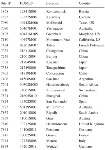
Table 2 SLR stations that tracked GPS and GLONASS satellites

dur-ing 2008

Site ID DOMES Location Country

1868 12341S001 Komsomolsk Russia

1893 12337S006 Katzively Ukraine

7080 40442M006 McDonald Texas, US

7090 50107M001 Yarragadee Australia 7105 40451M105 Greenbelt Maryland, US 7110 40497M001 Monument Peak California, US 7124 92201M007 Tahiti French Polynesia

7237 21611S001 Changchun China

7249 21601S004 Beijing China

7308 21704S002 Koganei Japan

7358 21749S001 Tanegashima Japan

7405 41719M001 Concepcion Chile

7406 41508S003 San Juan Argentina

7501 30302M003 Hartebeesthoek South Africa 7810 14001S007 Zimmerwald Switzerland

7821 21605S010 Shanghai China

7824 13402S007 San Fernando Spain 7825 50119S003 Mt. Stromlo Australia

7832 20101S001 Riyadh Saudi Arabia

7839 11001S002 Graz Austria

7840 13212S001 Herstmonceux United Kingdom

7841 14106S011 Potsdam Germany 7845 10002S002 Grasse France 7941 12734S008 Matera Italy 8834 14201S018 Wettzell Germany 0 200 400 600 800 1000 1200 1400 1600 1800 2000 # SLR observations

Number of SLR observations per station and satellite

G05 G06 R15 R24

Fig. 1 Number of SLR observations to GPS and GLONASS satellites

for 2008 (only those GLONASS satellites tracked the entire year 2008 are included)

many sites with only few observations: Six sites collected less than 100 NP and another six sites less than 500 NP. Only eight sites collected more than 1,000 NP. Consequently, the number of sites providing a strong contribution for the

combi-nation is limited to about 13–19. Figure2shows the network of the ILRS tracking sites. The number of SLR observations of each individual site is indicated by the size of the sym-bol. As usual, the SLR network geometry is far from being ideal, because most sites are located on the Northern hemi-sphere (about 75%). The number of observations, however, is about the same in both hemispheres: few Southern SLR sites provide altogether 15,051 NP, i.e., almost half of the observations.

The relatively small number of NP for the two GLON-ASS satellites R07 and R11 (see Table1) is explained by the fact that they were tracked only for about half of the year. The much larger number of GLONASS NP is explained by the larger LRA and a larger return signal strength (Pearlman 2009).

2.1.2 Analysis of SLR residuals

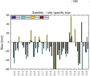
From the pure SLR range residual analysis described in Sect.2.1.1, the mean biases per station and satellite are shown in Fig.3for those stations with more than 100 NP in total during 2008 and for those satellites tracked the entire year. The corresponding RMS of the unbiased residuals are shown in Fig.4.

All stations show a mean bias for the SLR residuals of about−1 to −3cm, except for the station Katzively (1893). The weekly ILRS Combined Range Bias Reports (Gurtner 2009) reveal large biases for the observations to both LAG-EOS satellites for the station Katzively. The bias seen in Fig.3

is therefore not astonishing.

The mean biases in Fig.3differ considerably for the indi-vidual stations, although most of the mean biases are neg-ative. This is confirmed by the mean values provided for each satellite in Table 1. The mean biases per satellite of up to −2.5cm reveal that there are significant discrepan-cies between the GNSS microwave-based orbits, the SLR site positions according to SLRF2005 and the SLR range observations. These discrepancies have to be handled in the combined SLR-GNSS analysis, either by estimating bias parameters or by applying a priori biases (if known).

Figure4shows that the RMS is of the order of 2–4 cm. The same figure also shows that the RMS for GLONASS satellites is larger than for GPS satellites for most of the sites (see also RMS values in Table1).

The size of the mean biases and the RMS values reported here agree well with earlier studies carried out over time spans longer than one year, e.g., byFlohrer(2008).

2.1.3 Range bias estimation

As already stated in Sect.1, SLR observations may be biased. In the analysis the biases are usually absorbed by additional station-specific parameters, the so-called range biases. There

Fig. 2 Network of SLR sites.

The size of the marker indicates the number of SLR

observations. Those sites marked with blue circles have no co-location with GNSS (in our solution) −180 −120 −60 0 60 120 180 −90 −60 −30 0 30 60 90 −60 −40 −20 0 20 40 60 Bias [mm]

Satellite− / site−specific bias

G05 G06 R15 R24

Fig. 3 Mean site- and satellite-specific bias of SLR residuals for 2008.

The stations are sorted according to their total amount of SLR obser-vations, and stations with less than 100 NP are omitted. Only those GLONASS satellites tracked the entire year 2008 are included

0 10 20 30 40 50 60 RMS [mm]

Satellite− / site−specific RMS of SLR residuals

G05 G06 R15 R24

Fig. 4 RMS of site- and satellite-specific SLR residuals for 2008. The

stations are sorted according to their total amount of SLR observations, and stations with less than 100 NP are omitted. Only those GLONASS satellites tracked the entire year 2008 are included

are clearly defined guidelines within the ILRS, for which sta-tions range biases have to be estimated for observasta-tions to LAGEOS and ETALON. There are no such guidelines, how-ever, for SLR observations to GNSS satellites. For LAGEOS and ETALON the core sites are assumed to deliver unbiased observations. But this might not be true for observations to GNSS satellites, as the distance to the satellite and the char-acteristics of the retro-reflectors are two major facts influenc-ing the SLR range bias. Consequently, we cannot simply take over the strategy for observations to LAGEOS and ETALON. It is not clear which SLR sites deliver biased observations to GNSS satellites.Otsubo et al.(2001) state that SLR observa-tions to GNSS satellites of nearly all staobserva-tions may be biased. Therefore, we decided to set up range bias parameters for all SLR stations.

The second aspect to be studied is the satellite-dependency of the range biases. From the technical point of view there should be no difference between range biases for satellites carrying the same LRA and are located at the same orbital height. As a consequence, the range biases to all GLONASS satellites tracked in 2008 should be the same implying that one range bias parameter per station for all GLONASS sat-ellites should be sufficient. The same holds for range biases to the two GPS satellites. We might even go one step further and assume that the range biases to all GNSS satellites are identical for one SLR site.

The number of SLR observations per station is critical in this context. Due to the limited number of SLR observations to GNSS satellites (see Fig.1), a common range bias for all GNSS satellites per station is preferable in order to stabilize the solution. One has, however, to study first whether a com-mon range bias per station for all GNSS satellites may be justified. As we do not know the correct answer yet and the best method, we decided to test the different options already mentioned earlier:

– Satellite-dependent: one range bias parameter for each satellite;

– System-dependent: one range bias parameter for all GPS satellites, one for all GLONASS satellites;

– Per station: one range bias parameter for all GPS and GLONASS satellites together.

In all cases, the SLR range biases are set up individually for every station.

The range bias parameters in our solutions do not only account for the real range bias in the sense of SLR track-ing technology, but contain in addition the error in the LRA offsets, as we do not estimate a correction for these offsets. 2.2 Processing of GNSS data

The GNSS data were processed with the current strategies of the CODE Analysis Center of the IGS (Dach et al. 2009), with the exception that we did not generate 3-day orbital arcs, but 1-day arcs. GPS and GLONASS observations are analyzed together in a rigorous way, i.e., GPS and GLONASS orbits emerge from the same program run. The inclusion of GLONASS in the microwave analysis is of particular impor-tance for the combination of GNSS and SLR data: Figure1

and Table1 show that three GLONASS satellites and only two GPS satellites were observed by SLR and that, moreover, the number of SLR observations to GLONASS equals about twice the number of SLR observations to GPS satellites.

Modeling the GNSS antenna phase center is particularly difficult because the corresponding parameters are strongly correlated with the scale. The SAO and PCV for the sat-ellites as well as the absolute phase center models for the ground antennas were taken from the IGS standards (file igs05.atx, Schmid et al. (2007)). The phase center model for the GLONASS antennas in igs05.atx were, however, not derived together with the model for the GPS antennas. There-fore,Dach et al.(2010) performed a reprocessing to obtain SAO and PCV for GLONASS antennas that are consistent to the phase center model for GPS antennas. As these studies revealed discrepancies of up to 20 cm w.r.t. igs05.atx, SAO and PCV parameters were set up in the daily NEQ of our study. This allows it to either estimate corrections or fix the parameters to the a priori values (igs05.atx).

3 Inter-technique combination

The daily NEQ generated from SLR and GNSS data (see Sects.2.1and2.2, respectively) were in a first step stacked in order to obtain daily combined NEQ. Common parame-ters are ERP, geocenter coordinates and GNSS satellite orbit parameters.

When combining observations of the same type, but made with different instruments, e.g., with standard deviations of

σ1andσ2, the second NEQ contribution should be weighted

according to the ratio σ₁2/σ₂2. When combining the NEQs associated with the SLR and the GNSS techniques, respec-tively, the NEQs should be combined, e.g., according to NEQcomb= NEQG N S S+

σ2

G N S S

σ2

S L R

· NEQS L R (1) by applying the above formula to the normal equation matrix as well as to the vector of the right hand side.

AsσG N S S≈ 1−3mm (L1 phase observable) and σS L R ≈ 3−5mm (SLR normal points), the weight ratio would be

σS L R/σG N S S≈ 1−5 (2)

We used a value of 1 for the above ratio to generate the results presented here. A more refined analysis, based on a variance component estimation, should take into account instrument-specific and technique-instrument-specific weight ratios.

All daily combined NEQ for the year 2008 are then accu-mulated in order to derive a yearly solution. The orbit param-eters as well as the geocenter coordinates are pre-eliminated in this step from the NEQ but without constraining (solely the stochastic pulses are slightly constrained, see Sect.2). In this way they remain implicitly as free daily parameters. As it is not possible to get reliable estimates for station velocities from only one year of data, the a priori velocities provided by the technique-specific realizations of ITRF2005 (i.e., IGS05 and SLRF2005 for GNSS and SLR, respectively) are applied, but no velocity parameters are estimated. In order to pro-duce a yearly solution, the constraints necessary for remov-ing the rank deficiency of the NEQ are applied. We applied no-net-rotation (NNR) and no-net-translation (NNT) con-ditions for a selected subset of the IGS05 reference sites. The NNT conditions are needed as we estimate geocenter coordinates.

It is one of our goals to show that the combination of GNSS and SLR at the satellite level is equivalent to the combina-tion on the ground, i.e., at the stacombina-tion level. Therefore, we did not apply any local ties for the combined solutions. Conse-quently, as the SLR sites are neither included in the datum definition nor directly tied to the co-located GNSS sites, the station coordinates of the SLR sites are solely determined via the satellite co-locations.

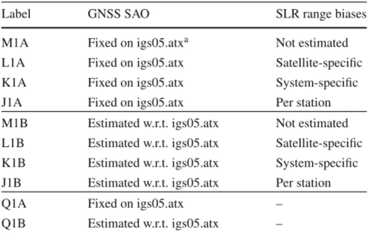
Several types of combined solutions are generated in order to answer the questions raised in Sect.1. Table3gives an overview of all combined solutions. The solutions differ in the way of handling of the GNSS SAO parameters and the estimation of SLR range biases (see Sect.2.1.3). If the SAO parameters are fixed, GNSS has no rank deficiency related to the scale. The scale of the combined solution will therefore be a weighted mean of the GNSS and SLR scale information. In the second case, if GNSS SAO are estimated, GNSS cannot contribute to the scale determination implying that the scale of these combined solutions will be defined solely by SLR.

Table 3 Overview of solutions generated

Label GNSS SAO SLR range biases

M1A Fixed on igs05.atxa Not estimated L1A Fixed on igs05.atx Satellite-specific K1A Fixed on igs05.atx System-specific J1A Fixed on igs05.atx Per station M1B Estimated w.r.t. igs05.atx Not estimated L1B Estimated w.r.t. igs05.atx Satellite-specific K1B Estimated w.r.t. igs05.atx System-specific J1B Estimated w.r.t. igs05.atx Per station

Q1A Fixed on igs05.atx –

Q1B Estimated w.r.t. igs05.atx – Upper part: combined solutions with fixed GNSS SAO; Middle part: combined solutions with estimated GNSS SAO; Lower part: GNSS-only solutions

a_{seeftp://igscb.jpl.nasa.gov/pub/station/general/igs05.atx}

The lower part in Table3lists GNSS-only solutions. They were generated for comparison purposes. One solution with SAO fixed to igs05.atx, and a second one where the SAO are estimated and the scale of the network is fixed to the IGS05 TRF by applying a no-net-scale condition.

After generating the yearly solutions, we performed a back-substitution of the yearly estimates into the daily com-bined NEQ in order to obtain daily solutions. The idea behind this procedure is to obtain reliable values for the SLR range biases. Normally, there are only few SLR observation avail-able per day (fewer than ten NP per station and satellite), which is why it is not possible to estimate range biases from daily solutions or solutions based on few days only. As a range bias is not expected to change with time if there were no changes at the station (or satellite), yearly range bias esti-mates are reasonable and can be introduced as known values into the daily solutions. Apart from the range biases, the ERP and GNSS SAO (if estimated) are introduced from the yearly solution and fixed as well. Station coordinates of the yearly solutions are tightly constrained for the 117 IGS core sites and for the SLR sites with more than 250 NP in 2008 (i.e., 16 sites), and only loosely constrained for the remaining SLR sites. The main parameters of interest of the daily solutions derived from the back-substitution are the geocenter coor-dinates and the orbit parameters. Both parameter types are estimated without constraints.

4 Results

4.1 Terrestrial reference frame: station coordinates

The datum definition for the combined solution is done by applying NNR and NNT conditions over a sub-set of GNSS

sites (see Sect. 3). The network of SLR sites is appended only via the satellite co-locations. Consequently, as no local ties are applied, the station coordinates of the SLR sites are estimated as free parameters and are not directly linked to the GNSS site coordinates. For validation the estimated SLR coordinates are either compared directly with the a priori TRF, or the coordinate differences w.r.t. the estimated GNSS station coordinates are compared with the official local ties. The latter method is an indirect way to check the coor-dinate estimates for co-located GNSS-SLR sites for which the local ties are available. Almost all SLR sites included in our study are co-located with a GNSS site (see Fig.2). The only exceptions are San Juan (7406), Riyadh (7832) and Changchun (7237). The GNSS sites were not included in our analysis for the latter two sites, and San Juan does not have an IGS site.

4.1.1 Impact of using only one year of data

Independent of whether we validate the estimated SLR sta-tion coordinates indirectly (via local ties to GNSS sites) or directly (by comparison with SLRF2005), we must keep in mind that the solutions are based only on one year of data. We thus fully rely on the uncertainty of the velocities given in the a priori TRF (see Sect.3). We must, moreover, keep in mind that the data set used here was not included in the ITRF2005 computations and is far away from the reference epoch of the ITRF2005 (i.e, January 1st, 2000) and most of the local tie measurements. Consequently, we cannot expect a perfect agreement of the SLR station coordinates derived from our solutions with the a priori TRF and the local ties.

The question arises, however, which level of agreement can be achieved for the SLR station coordinates if we use only one year of data. In order to answer this question, we compute two single-technique solutions for the year 2008, i.e., one GNSS-only solution and one SLR-only solution (using LAGEOS data), both with a well-defined datum (i.e., applying NNR and NNT conditions for a subset of verified reference sites). The method of computing the GNSS-only solution does not differ from the combined solution (except for the fact that it is a GNSS-only solution). The SLR-only solution is, however, different: well-defined datum condi-tions are applied, whereas the station coordinates are fully free in the combined solution. The SLR solutions based on observations to LAGEOS are more stable because of the much larger amount of data. Subsequently, the coordinate dif-ferences between the co-located GNSS-SLR sites are com-puted from the resulting estimated yearly station coordinates and compared to the local ties. The discrepancies are shown in Fig.5. Obviously, the level of agreement reached by the annual solution is about 1–2 cm. For comparison, the dis-crepancies between the local ties and the IGS and ILRS input solutions for the ITRF2008 computations performed at DGFI

Fig. 5 Comparison of local ties with the coordinate differences

between co-located GNSS-SLR sites derived from estimated station coordinates (absolute values of the differences): GNSS and SLR single-technique solutions for 2008 generated with the Bernese GPS Software and ITRF2008 input solutions provided by the IGS and ILRS

(Seitz et al. 2010) are provided, as well. As mentioned, it is not amazing that the discrepancies for our annual solutions are larger than for the long-term solutions for ITRF2008. The differences are, however, small for most co-locations. There-fore, it is justified to perform the case studies based on only one year of data.

4.1.2 Comparison with SLRF2005

One important question to be answered by our studies is whether the connection between GNSS and SLR via com-mon orbit parameters only is sufficient, or do we need the connection on the ground (i.e., by introducing the local ties at co-located sites) in addition.

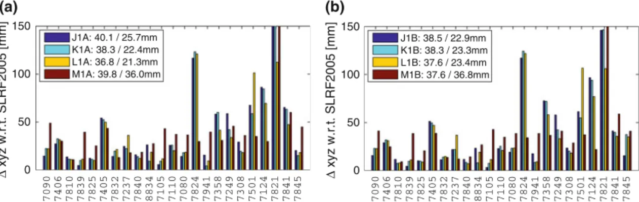
Figure6illustrates the direct coordinate comparison with SLRF2005 by showing the absolute values of the differences for the combined solutions labelled “A” (SAO fixed) and “B” (SAO estimated). The mean difference over all SLR sites

is about 36–40 mm, but the differences vary substantially from site to site. It is, however, clear that the mean value is highly influenced by the stations with large discrepan-cies, e.g., Shanghai (7821), San Fernando (7824), and Tahiti (7124). For some of them, the large discrepancies can be explained by the a priori TRF: Stations Shanghai (7821), Tanegashima (7358) and San Juan (7406) are new in the SLRF2005 implying that the coordinates and velocities in the SLRF2005 are only weakly determined and may not give a good position for the year 2008. A comparison with the upcoming ITRF2008 should result in more reliable differ-ences for these stations.

The stations are arranged in descending order of the total number of SLR observations (Fig.1). The station coordinates to the right are only weakly determined. Larger discrepan-cies are thus not surprising as no additional constraints were applied to the SLR station coordinates. As a consequence, the median of the differences are clearly smaller than the mean values, i.e., about 22 mm, except for the solution types “M” (i.e., no range biases estimated). For the latter the differences are significantly larger, indicating that an estimation of bias parameters is indispensable. The impact of different types of range bias estimation (solutions “J”, “K” and “L”) on the estimated station coordinates is on the level of a few millime-ters for most of the stations, independently of whether GNSS SAO are estimated or not.

The SLR coordinates of the corresponding solution types “A” (SAO fixed) and “B” (SAO estimated) agree well, inde-pendent of the set–up of range bias parameters. The mean difference is about 4 mm in vertical and 2 mm in horizon-tal direction. This behavior demonstrates that the common estimation of SLR range biases and GNSS SAO is feasible.

As most sites agree with the SLRF2005 at the level of about 22 mm we conclude that the connection of the SLR network to the GNSS network solely via the common orbit parameters (and ERP) is possible at the level of a few centi-meters. 0 50 100 150 (a) (b) Δ xyz w.r.t. SLRF2005 [mm] 7090 7406 7810 7839 7825 7405 7832 7237 7840 8834 7105 7110 7080 7824 7941 7358 7249 7308 7501 7124 7821 7841 7845 J1A: 40.1 / 25.7mm K1A: 38.3 / 22.4mm L1A: 36.8 / 21.3mm M1A: 39.8 / 36.0mm 0 50 100 150 Δ xyz w.r.t. SLRF2005 [mm] 7090 7406 7810 7839 7825 7405 7832 7237 7840 8834 7105 7110 7080 7824 7941 7358 7249 7308 7501 7124 7821 7841 7845 J1B: 38.5 / 22.9mm K1B: 38.3 / 23.3mm L1B: 37.6 / 23.4mm M1B: 37.6 / 36.8mm

Fig. 6 Comparison of estimated SLR station coordinates with SLRF2005: absolute value of coordinate differences. The mean and median of the

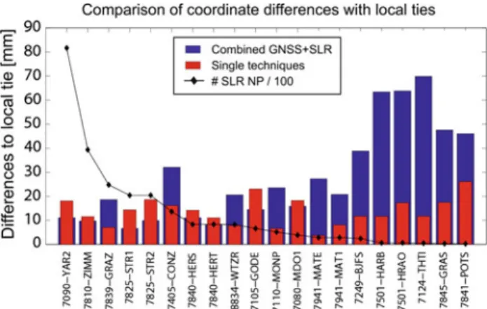
Fig. 7 Coordinate differences between co-located GNSS-SLR sites

derived from estimated station coordinates with local tie values (abso-lute values of the differences): combined solution “J1A” (SAO fixed; range biases per station) and single-technique solutions

4.1.3 Comparison with co-located GNSS sites

The indirect method, where the coordinate differences of the combined solution are compared to the local ties, is used as a second validation of the estimated SLR station coor-dinates. Figure7 shows the discrepancies for the solution type “J1A” as an example (SAO fixed; range biases per sta-tion). The comparisons for the other solution types of Table3

look similar. The discrepancies between the local ties and the coordinate differences derived from the single-technique solutions already seen in Fig.5are included for reference in Fig.7. The stations are arranged in descending order of the total amount of SLR observations to GNSS satellites. For the stations to the left and in the center part of the figure the agreement with the local ties is at the level of 1–2 cm. As the discrepancies for the single-technique solutions are on the same level, we conclude that a connection of the SLR sites to the GNSS network by using only the satellite co-locations works well.

The prerequisite for stable coordinate estimates is a suf-ficient number of SLR observations. According to Fig. 7

the minimum number of SLR observations needed to derive coordinate estimates as stable as for the single-technique solutions is about 250–300. The coordinate estimates for McDonald (7080) based on 388 observations still agree quite well, whereas the connection to the GNSS network for Matera (7941) with 285 observations is already clearly weaker than for the single-technique solutions, and Beijing (7249) with 245 observations seems to be connected very weakly. One has to keep in mind, however, that Beijing is an isolated location compared to Matera (see Fig.2). This fact weakens the position determination because of the poor observing geometry. The remaining sites in the rightmost part of Fig.7have fewer than 100 NP. The large discrepan-cies must be attributed to this fact.

Fig. 8 Coordinate differences between co-located GNSS-SLR sites

derived from estimated station coordinates with local tie values (abso-lute values of the differences): combined solutions “J1A” and “J1B” (see Table3). The stations are sorted in descending order according to the total amount of SLR observations

Disregarding those sites with only few observations, the SLR and GNSS coordinates estimated in the combined solu-tions (using satellite co-locasolu-tions only) agree better with the local ties than the coordinates estimated independently from single-technique solutions (based on a well-defined datum for the SLR solution, see Sect.4.1.1). This result indicates that the SLR network can be attached to the GNSS network by using only satellite co-locations.

We validated the SLR station coordinates indirectly via co-locations with GNSS sites (as described above) for all solu-tion types of Table3. Comparing the solution types with SAO parameters estimated (“B”) with the corresponding solution type, where the SAO were fixed (“A”), answers the ques-tion whether the SLR observaques-tions can provide the scale (for the combined solution) so that the GNSS SAO can be estimated without fixing the scale to the a priori TRF (see Sect.3). Figure8shows the two solution types for the case of SLR range biases estimated per station (i.e., “J1A” and “J1B”) as a typical example. The differences between the estimated GNSS and SLR station coordinates at co-located sites are not heavily influenced by estimating GNSS SAO parameters. For most sites the agreement with the official local ties is slightly better for the solution with estimating the GNSS SAO, indicating that the scale of the combined solution should be defined solely by SLR and not by a mix-ture between GNSS and SLR.

4.2 Reference frame: scale and geocenter

When discussing the scale definition it is necessary to study the impact of different solution strategies. In general, if the GNSS SAO parameters are fixed on their a priori values, the GNSS contribution provides information about the scale. Therefore, the scale of the combined solution is a weighted mean of the GNSS and SLR scale information, despite the

Table 4 Scale for the GNSS

reference sites between the different solution types of Table3[given in (ppb)]

M1A, L1A, K1A, J1A M1B, L1B, K1B, J1B Q1A

M1A, L1A, K1A, J1A 0.0 0.9 0.0

M1B, L1B, K1B, J1B 0.0 0.9

Q1B 0.0 0.2

IGS05 0.2 −0.7 0.2

fact that the GNSS contribution dominates the combined scale due to the larger and denser network providing a large amount of observations. GNSS contributions estimating GNSS SAO parameters have a rank deficiency concerning the scale. The combined solution therefore takes over the scale from the SLR contribution.

We compared all solution types in Table 3 by a seven-parameter similarity transformation using the GNSS reference sites. As expected, the translation and rotation parameters are negligible, because neither the range bias nor the GNSS SAO parameters are correlated with the orientation and translation of the network. The only parameter differing significantly from zero is the scale. Table4summarizes the scale differences of interest. No significant scale differences are present in the group of solutions with fixed GNSS SAO (labels “A”). The same is true for the solutions of type “B” (GNSS SAO estimated). The RMS of the coordinate resid-uals after the transformation is only about 0.03 mm for all these comparisons. We can thus conclude that the different types of SLR range bias estimation (labels “J”, “K”, “L”) have no significant impact on the scale of the combined net-work, independent of whether the GNSS SAO are estimated or not.

As there are no significant scale differences between the solution “M1B” (without range biases) and the other solu-tions of type “B”, we conclude that the estimation of range biases does not disturb the ability of SLR to deliver the scale information for the combined network.

The transformations between solutions with fixed GNSS SAO and with estimated GNSS SAO, i.e., types “A” and “B”, respectively, show a scale difference of 0.9 ppb in all cases, implying that the scale information from SLR dif-fers by 0.9 ppb from the scale information resulting from a weighted mean of SLR and GNSS. The RMS of the coordi-nate residuals for these comparisons is about 0.3 mm.

The rightmost column in Table4shows the scale differ-ences compared to a GNSS-only solution with SAO fixed on the igs05.atx values. The scale differences to the solution types “B” (SAO estimated) are identical to the differences between the combined solution types, i.e., 0.9 ppb. We thus conclude that the scale of the combined solution is mainly driven by GNSS, if no SAO are estimated.

Let us briefly look at the geocenter coordinates— without expecting an improvement (see Sect.1). Daily geo-center coordinates are derived from a back-substitution of the

Table 5 Daily geocenter coordinates: Mean and RMS

Solution type Mean ( mm) RMS ( mm)

X Y Z X Y Z Q1A 5.7 1.6 −1.4 5.1 4.4 8.1 M1A 6.7 1.2 2.1 7.4 4.6 10.0 K1A 5.5 1.6 −1.5 5.9 4.7 8.3 J1A 5.5 1.6 −1.6 5.9 4.6 8.5 M1B 8.0 1.7 6.5 7.3 4.4 9.8 K1B 6.7 2.1 2.8 5.7 4.4 8.2 J1B 6.7 2.1 2.7 5.7 4.4 8.3

annual solutions (see Sect.3). Table5lists the mean geocen-ter coordinates and the scatgeocen-ter for the year 2008 for several solution types. Comparing the GNSS-only solutions with the combined solutions confirms our prediction that SLR obser-vations to GNSS satellites cannot stabilize the geocenter.

The RMS of the daily geocenter coordinates is larger for the solution types without range bias estimation (i.e., types “M”), indicating the necessity of estimating or applying range biases.

One might have the impression that the RMS of the other combined solutions increases slightly compared to the GNSS-only solution, mainly the x-component (i.e., from 5.1 mm to 5.7–5.9 mm). The varying SLR network geometry might explain this result. According to studies carried out by

Collilieux and Altamimi(2009), the x-component of the geo-center is the most sensitive component. But as stated earlier, the inclusion of LAGEOS data is required for performing a precise study of the geocenter coordinates.

4.3 GNSS satellite antenna offsets

Figure9shows the estimated corrections for the GNSS SAO in z-direction w.r.t. the values given in igs05.atx. The mean corrections for all GPS and GLONASS satellites of the com-bined solutions are about 119 and -13 mm, respectively.

As mentioned, the SAO in z-direction is correlated with the scale of the network. According toZhu et al.(2003) the correlation is given by:

0 10 20 30 40 50 60 70 −400 −300 −200 −100 0 100 200 Satellite number Δ SAO Z w.r.t. igs05.atx [mm] M1B J1B K1B L1B Q1B

Fig. 9 Estimated corrections for GNSS SAO (z-component) w.r.t.

igs05.atx. Satellite numbers for GLONASS are shifted by +40 (the

vertical line separates the GPS and GLONASS satellites). Mean

cor-rections for GPS and GLONASS of the combined solutions are 119 and −13mm, respectively

Consequently, the mean correction for the GPS satellites corresponds to a scale difference of about 0.9 ppb, confirming the results of Table4. The mean SAO correction for GLON-ASS is smaller, but as GPS dominates the GNSS part due to more satellites and more stations, the scale differences seen in Table4are driven mainly by the GPS part.

Furthermore, differences between the GNSS-only solu-tion (“Q1B”, using no-net-scale condisolu-tion w.r.t. IGS05 TRF) and the combined solutions can be clearly seen in Fig.9. On average, the differences are 82 mm and 76 mm for the GPS and GLONASS satellites, respectively. According to Eq. (3), this difference in SAO corresponds to a scale differ-ence of about 0.6 ppb. This indicates that there are significant differences between the scale of IGS05 (that was fixed for the GNSS-only solution) and the scale given by SLR in the combined solutions. This difference may be understood as the IGS05 was derived using the old relative antenna phase center model of the IGS.

A comparison of different combined solutions does not show significant differences in the SAO estimates. If we take the solution “M1B” as a reference (as there were no SLR range biases estimated), the SAO estimates of the other com-bined solutions of type “B” differ in average by only 1 mm. Therefore we conclude that the estimation of SLR range biases has no significant impact on the estimation of GNSS SAO. This result confirms the statement made in Sect.4.1, that a common estimation of GNSS SAO and SLR range biases is possible.

This conclusion is confirmed by the fact that the mean SAO correction for the GPS and GLONASS satellites are substantially different. If there would be a one-to-one corre-lation between GNSS SAO and SLR range biases, the NEQ

would have a singularity regarding the scale. This would lead to identical GNSS SAO corrections for all satellites due to the correlation between scale and GNSS SAO according to Eq. (3).

Range biases and GNSS SAO can be de-correlated because of their different characteristics. Range biases have the same size for all directions of the observations (i.e. inde-pendent of azimuth and elevation angles), whereas the impact of the GNSS SAO on the observations depend on the location in the satellite-fixed system. As a consequence, the partial for a range bias parameter is 1, whereas the partial for the SAO in z-direction is cos(α), with α being the nadir angle of the observation.

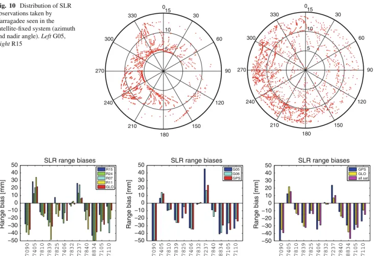
If we look at the distribution of the SLR observations seen in the satellite-fixed system (given by the nadir and azimuth angles) we can evaluate whether the correlation between GNSS SAO in z-direction and SLR range biases can be reduced. Figure10shows, as typical examples, the distribution of SLR observations for the station Yarraga-dee to the GPS satellite G05 and the GLONASS satel-lite R15 as seen from the satelsatel-lite. The distribution is quite well for GLONASS so that the correlation is clearly reduced. For GPS satellites the distribution is not as homo-geneous. GPS satellites follow the same ground track every day implying that the observation geometry is the same every day. Nevertheless, a de-correlation should be possi-ble, because all stations are contributing to the estimation of the SAO.

4.4 SLR range biases

As mentioned in Sect.2.1.3it is not yet really clear what is the best method for estimating SLR range biases to GNSS satellites. The estimated bias parameters for solution types “B” (SAO estimated) shown in Fig.11seem to indicate that the observations of all stations are biased. There might be only one exception, namely the station Riyadh (7832). The estimated bias parameters are up to a few centimeters. They have the same order of magnitude as that seen in the anal-ysis of pure SLR residuals shown in Fig.3. Therefore we conclude that the fixed station coordinates, orbits and ERP are not the source for the discrepancies in Fig.3, because the three parameter types are estimated in the solutions shown in Fig.11. The discrepancy is more likely due to errors or uncer-tainties in the observation models. As already mentioned in Sect.2.1.3the estimated bias parameters account for both, i.e., range biases and errors in the LRA offsets. As SLR range observations normally are not biased by a few centimeters, we conclude that the estimated bias parameters mainly con-tain the effect of errors in the LRA offsets rather than real range biases.

Figure11also shows that the differences between satellite-specific, system-specific and station-specific biases are small

Fig. 10 Distribution of SLR

observations taken by Yarragadee seen in the satellite-fixed system (azimuth and nadir angle). Left G05,

Right R15 5 10 15 30 210 60 240 90 270 120 300 150 330 180 0 5 10 15 30 210 60 240 90 270 120 300 150 330 180 0 −50 −40 −30 −20 −10 0 10 20 30 40 50 Range bias [mm] SLR range biases R15 R24 R07 R11 GLO −50 −40 −30 −20 −10 0 10 20 30 40 50 Range bias [mm] SLR range biases G05 G06 GPS −50 −40 −30 −20 −10 0 10 20 30 40 50 Range bias [mm] SLR range biases GPS GLO all sat

Fig. 11 Comparison of range bias estimates (solutions labelled “B” in Table3). Left satellite-specific vs. system-specific for GLONASS satellites,

Middle satellite-specific versus system-specific for GPS satellites, Right system-specific versus station-specific

−50 −40 −30 −20 −10 0 10 20 30 40 50 Range bias [mm]

SLR range biases for satellite R15

GNSS SAO fixed GNSS SAO estimated −50 −40 −30 −20 −10 0 10 20 30 40 50 Range bias [mm]

SLR range biases for GLONASS satellites GNSS SAO fixed GNSS SAO estimated −50 −40 −30 −20 −10 0 10 20 30 40 50 Range bias [mm]

SLR range biases for all satellites GNSS SAO fixed GNSS SAO estimated

Fig. 12 Impact of estimating GNSS SAO on the SLR range bias parameters for satellite-specific (left), system-specific (middle) and station-specific

range biases (right) for solution types “A” (SAO fixed) versus “B” (SAO estimated) in Table3

compared to the absolute value of the bias for most of the stations. Consequently, we conclude that a common bias parameter for all GPS and GLONASS satellites per station is sufficient. This reduction of the number of parameters is highly desired, in particular for sites with a small number of SLR observations. However, further studies are needed in this field, especially in view of a distinction between errors in the LRA offsets and real SLR range biases.

Figure12shows that the impact of estimating GNSS SAO on the range biases is small, independent of whether the range biases are estimated as one parameter per station, as system-dependent or as satellite-dependent parameters. The differences are only a few millimeters at maximum. The mean differences over all stations are provided in Table6. They are about 1 mm in most cases. We have also seen that the impact of estimating SLR range biases on the estimated

Table 6 Mean difference in SLR range biases when estimating GNSS

SAO [given in (mm)]

G05 G06 R15 R24 R07 R11 GPS GLO All

1.3 1.0 −2.9 5.1 2.5 0.4 0.9 1.1 1.5

Column 1–6: satellite-specific range biases; column 7–8: system-specific range biases; column 9: one range bias per station

GNSS SAO is only 1 mm in average, as well (see Sect.4.3). These results underline that the common estimation of range biases and GNSS SAO is possible. The remaining correla-tion between range biases and GNSS SAO (due to unevenly distributed observations) has an impact on the estimated bias parameters and GNSS SAO parameters of 1 mm at maximum.

4.5 Satellite orbits

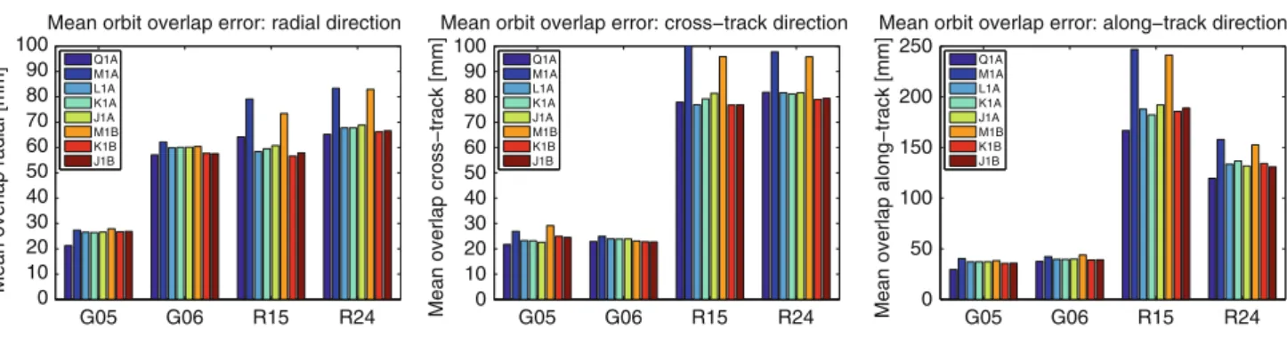
The orbits emerging from the combined solutions are derived from a back-substitution of the annual solutions (see Sect.3). The mismatch of the daily orbits at the day boundaries is an important criterion. We compared consecutive daily orbi-tal arcs at midnight and computed the discrepancy in radial, along-track and cross-track direction. Figure13shows the mean discrepancy in the three components for several solu-tion types.

Although one would expect the radial component to be the major component for which the inclusion of SLR would have an impact, we can recognize that the other components show differences as well. First, we can see that the impact of different solution strategies is larger for the GLONASS satellites than for the GPS satellites. In general, the solution types without considering SLR range biases (“M”) show a clear degradation of the orbital fit at the day boundaries. As the estimated bias parameters are different from zero (see Sect.4.4) it is not a surprise that neglecting such biases leads to a degradation of the combined solution. This behavior confirms the conclusion that SLR range biases have to be considered.

Only the GLONASS satellites show smaller orbit overlap errors in the combined solution (with range biases consid-ered) than in the GNSS-only solution, showing that the SLR observations to the GLONASS satellites—despite the lim-ited amount of data—slightly improve the orbits compared to a GNSS-only solution.

Figure13also shows that the estimation of GNSS SAO parameters slightly reduces the orbit overlap error in nearly all cases. This is a further indication that the SAO values according to igs05.atx need to be updated.

5 Conclusions and outlook

We performed a combination of GNSS and SLR observa-tions for one year of data using the satellite co-locaobserva-tions at the GPS and GLONASS satellites. This method is a direct way to combine GNSS and SLR observations as common orbit parameters provide a strong link between both tech-niques.

The agreement of the estimated SLR coordinates with the a priori TRF is on the level of 2 cm for stations with a reason-able number of observations. The agreement with the GNSS site coordinates corrected by the local ties is at the level of 1–2 cm for stations with a reasonable number of observa-tions. This level of agreement is only slightly worse than that achieved for long-term single-technique solutions (derived, e.g., for ITRF2008).

A minimum number of SLR observations is required, however. We conclude that an amount of 250–300 NP is sufficient for stable coordinate estimates without introduc-ing the local ties as additional constraints. The GNSS-SLR combination using solely the satellite co-locations therefore allows for an independent control of the local ties, if a min-imum number of SLR observations is available. It is clear, however, that the additional use of the local ties stabilizes the solutions, provided that only the reliable local ties are used.

Independent of whether we connect GNSS and SLR at the stations (by introducing local ties) or at the GNSS

sat-G05 G06 R15 R24 0 10 20 30 40 50 60 70 80 90 100

Mean overlap radial [mm]

Mean orbit overlap error: radial direction

Q1A M1A L1A K1A J1A M1B K1B J1B G05 G06 R15 R24 0 10 20 30 40 50 60 70 80 90 100

Mean overlap cross−track [mm]

Mean orbit overlap error: cross−track direction

Q1A M1A L1A K1A J1A M1B K1B J1B G05 G06 R15 R24 0 50 100 150 200 250

Mean overlap along−track [mm]

Mean orbit overlap error: along−track direction

Q1A M1A L1A K1A J1A M1B K1B J1B

Fig. 13 Mean orbit overlap errors at day boundaries. Only those satellites tracked the entire year 2008 are displayed. Note the different scale of

ellites (by estimating common orbit parameters), we have to know the connecting vector between the GNSS and SLR reference points as accurate as possible. The connecting vec-tors on ground are the local ties—with problems discussed in many other publications. We therefore took the second way and made use of the connection at the satellites. When fol-lowing this way we have to know two vectors, namely the vector from the GNSS antenna phase center to the satellite’s center of mass (CoM) and the vector from the LRA to the CoM. Both vectors have to be known accurately. Many stud-ies suggest that this assumption is not yet met. The problems related to the location of the GNSS antenna phase center are well known. We decided to avoid this uncertainty by esti-mating the SAO parameters. The second connecting vector (between LRA and CoM) was assumed to be provided cor-rectly, although this might not be the case. The errors in the LRA offsets are absorbed by the SLR range biases in our studies. The estimated range biases are in the order of a few centimeters for most sites. As the SLR measurements are accurate to a few millimeters, the major part of the estimates must be attributed to the errors in the LRA offsets. Investi-gations of the LRA offsets are highly desired but they would clearly need a longer time span of data.

The ability of determining the geocenter by SLR observa-tions depends on the satellite analyzed. In the case of spher-ical satellites (e.g., LAGEOS), the modeling of the forces acting on the satellite is simple and needs only few parame-ters, which is why the geocenter estimates are reliable and do not contain artefacts from insufficiently modeled effects of solar radiation pressure. In the case of GNSS satellites, the geocenter estimates are weakened by the need to model the solar radiation pressure by estimating parameters. It would be worthwhile to extend the studies presented here by addi-tionally using SLR observations to LAGEOS-type satellites in order to stabilize the geocenter. As a side effect, such an extension would stabilize the coordinate estimates of the SLR sites due to a much larger amount of data.

The ability to determine the scale is due to the SLR tech-nique itself. We showed that the scale of SLR is transferred well to the GNSS network if both observing techniques are combined via the satellite co-locations.

SLR range biases and GNSS SAO can be estimated together due to a good distribution of the SLR observations w.r.t. the nadir angle at the satellite.

This study revealed that the SLR range biases can be esti-mated for GNSS satellites as one parameter per station. A distinction between individual GNSS satellites is not neces-sary as the differences are small compared to the estimated bias parameters. This is important in particular because of the small amount of SLR observations per satellite for many stations. Further studies related to this topic are required. It would in particular be helpful to use a longer time span of data and to include observations to LAGEOS, as there are

clear definitions for the range biases. As already explained in this section, the estimates for the range biases presented here contain the errors of the LRA offsets as well. If the LRA offsets are considered to be the major error source, a bias parameter per satellite should be more appropriate than a bias parameter per station. A testing facility for LRA as it is proposed byDell’Agnello et al.(2010) can improve the understanding of the behavior of different types of LRA. This will help to better model the SLR range biases and, thus, separate their effect from errors in the LRA offsets. The importance of correctly modeling the SLR range biases has been already emphasized byCoulot et al.(2009). The neces-sity to consider SLR range biases in the combined analysis is confirmed by the orbit overlap errors, too. The mismatch at the day boundaries increases when neglecting the biases. But if the biases are taken into account, the overlap errors are reduced, especially for the GLONASS satellites.

GNSS satellite clock parameters are also correlated with the scale and SAO parameters. This aspect was not yet studied.

The studies performed here have to be extended to a longer time span of data. GLONASS data from May 2003 onwards have already been reprocessed at CODE and combined GPS-GLONASS NEQ are already available (Dach et al. 2010). SLR tracking data is available for the two GPS satellites and for several GLONASS satellites. Such an extension of the study will allow for the determination of more reliable val-ues for the GNSS SAO. The results have the potential to contribute to an update of the official values within the IGS. The updated values would then be consistent with the scale information from SLR what is not the case today.

Acknowledgments The work was done within CODE, a joint

ven-ture of the Astronomical Institute of the University of Bern (AIUB), the Swiss Federal Office of Topography (swisstopo), the Federal Agency for Cartography and Geodesy (BKG), and the Institut für Astronomische und Physikalische Geodäsie of the Technische Universität München (IAPG/TUM). The ILRS (Pearlman et al. 2002) and IGS (Dow et al. 2009) are acknowledged for providing space-geodetic data.

References

Altamimi Z, Collilieux X, Legrand J, Garayt B, Boucher C (2007) ITRF2005: a new release of the international terrestrial reference frame based on time series of station positions and earth orien-tation parameters. J Geophys Res 112(B9):401ff. doi:10.1029/ 2007JB004949

Appleby G, Otsubo T (2000) Comparison of SLR measurements and orbits with GLONASS and GPS microwave orbits. In: Proceed-ings of the 12th international workshop on laser ranging, Matera, Italy

Beutler G, Brockmann E, Gurtner W, Hugentobler U, Mervart L, Rothacher M (1994) Extended orbit modeling techniques at the CODE processing center of the international GPS service (IGS): theory and initial results. Manuscr Geod 19:367–386

Brockmann E (1997) Combination of solutions for geodetic and geody-namic applications of the global positioning system (GPS). Geod Geophys Arb in der Schweiz 55, Zürich, Switzerland

Collilieux X, Altamimi Z, Coulot D, Ray J, Sillard P (2007) Com-parison of very long baseline interferometry, GPS, and satellite laser ranging height residuals from ITRF2005 using spectral and correlation methods. J Geophys Res 112:B12403. doi:10.1029/ 2007JB004933

Collilieux X, Altamimi Z (2009) Impact of the network effect on the origin and scale: case study of satellite laser ranging. In: Sideris M (ed) Observing our changing earth. Proceedings of the 2007 IAG general assembly, Perugia, Italy. IAG Symp 133:31–38

Coulot D, Berio P, Bonnefond P, Exertier P, Feraudy D, Laurain O, Deleflie F (2009) Satellite laser ranging biases and terrestrial refer-ence frame scale factor. In: Sideris M (ed) Observing our changing earth. Proceedings of the 2007 IAG General Assembly, Perugia, Italy. IAG Symp 133:39–46

Dach R, Hugentobler U, Fridez P, Meindl M (eds) (2007) Bernese GPS software version 5.0. Astronomical Institute, University of Bern, Bern, Switzerland

Dach R, Brockmann E, Schaer S, Beutler G, Meindl M, Prange L, Bock H, Jäggi A, Ostini L (2009) GNSS processing at CODE: status report. J Geod 83(3–4):353–365. doi:10.1007/ s00190-008-0281-2

Dach R, Schmid R, Schmitz M, Thaller D, Schaer S, Lutz S, Stei-genberger P, Wübbena G, Beutler G (2010) Improved antenna phase center models for GLONASS. GPS Sol. doi:10.1007/ s10291-010-0169-5

Dell’Agnello S, Delle Monache GO, Currie DG, Vittori R, Cantone C, Garattini M, Boni A, Martini M, Lops C, Intaglietta N, Tauraso R, Arnold DA, Pearlman MR, Bianco G, Zerbini S, Maiello M, Berardi S, Porcelli L, Alley CO, McGarry JF, Sciarretta C, Luceri V, Zagwodzki TW (2010) Creation of the new industry-standard space test of laser retroreflectors for the GNSS. Adv Space Res (Accepted for publication). doi:10.1016/j.asr.2010.10.022 Dow JM, Neilan RE, Rizos C (2009) The international GNSS service

in a changing landscape of global navigation satellite systems. J Geod 83(3–4):191–198. doi:10.1007/s00190-008-0300-3 Eanes R, Nerem R, Abusali P, Bamfort W, Key K, Ries J, Schutz B

(2000) GLONASS orbit determination at the Center for Space Research. In: Slater J, Noll C, Gowey K (eds) Proceedings of the international GLONASS experiment (IGEX-98) Workshop, IGS, Jet Propulsion Laboratory

Flohrer C (2008) Mutual validation of satellite-geodetic techniques and its impact on GNSS orbit modeling. Geod. Geophys. Arb. in der Schweiz 75, Zürich, Switzerland. ISBN: 978-3-908440-19-2 Ge M, Gendt G, Dick G, Zhang F, Reigber C (2005) Impact of GPS

satellite antenna offsets on scale changes in global network solu-tions. Geophys Res Lett 32:L06310. doi:10.1029/2004GL022224 Gurtner W (2009) ILRS combined range bias report (sent weekly via

slrmail)

Krügel M, Angermann D (2005) Analysis of local ties from multi-year solutions of different techniques. In: Richter B, Dick W, Schwegmann W (eds) Proceedings of the IERS workshop on site

co-locations, Verlag des Bundesamts für Kartographie und Geo-däsie, Frankfurt am Main, Germany, IERS technical note, no. 33 Lemoine FG, Zelensky NP, Chinn DS, Pavlis DE, Rowlands DD,

Beckley BD, Luthcke SB, Willis P, Ziebart M, Sibthorpe A, Boy JP, Luceri V (2010) Towards development of a consistent orbit series for TOPEX, Jason-1, and Jason-2. Adv Space Res 46(12):1513–1540. doi:10.1016/j.asr.2010.05.007

Otsubo T, Apleby G, Gibbs P (2001) GLONASS laser ranging accuracy with satellite signature effect. Surv Geophys 22:509–516 Pavlis E (1995) Comparison of GPS s/c orbits determined from GPS

and SLR tracking data. Adv Space Res 16(12):1255–1258. doi:10. 1016/0273-1177(95)98780-R

Pearlman MR (2009) Technology challenges for SLR ranging to GNSS satellites. In: Pavlis E (ed) International technical laser workshop on SLR tracking of GNSS constellations, position papers Pearlman MR, Degnan JJ, Bosworth JM (2002) The international laser

ranging service. Adv Space Res 30(2):125–143

Rothacher M (2003) Towards a rigorous combination of space geo-detic techniques. In: Richter B, Schwegmann W, Dick W (eds) Proceedings of the IERS workshop on combination research and global geophysical fluids. IERS technical note, no. 30, Bundesamt für Kartographie und Geodäsie, Frankfurt am Main

Schmid R, Steigenberger P, Gendt G, Ge M, Rothacher M (2007) Gen-eration of a consistent absolute phase center correction model for GPS receiver and satellite antennas. J Geod 81(12):781–798. doi:10.1007/s00190-007-0148-y

Seitz M, Angermann D, Blossfeld M, Gerstl M, Heinkelmann R, Kelm R, Müller H (2010) Die Berechnung des Internationalen Ter-restrischen Referenzrahmens ITRF2008 am DGFI. zfv 135(2): 73–79

Springer T (2000) Modelling and validating orbits and clocks using the global positioning system. Geod Geophys Arb in der Schweiz 60, Zürich, Switzerland

Thaller D (2008) Inter-technique combination based on homoge-neous normal equation systems including station coordinates, earth orientation and troposphere parameters. Scientific technical report STR08/15, Deutsches GeoForschungsZentrum Potsdam, Germany

Thaller D, Mareyen M, Dach R, Gurtner W, Beutler G, Richter B, Ihde J (2009) Preparing the bernese GPS software for the analysis of SLR observations to geodetic satellites. In: Schillak S (ed) Proceed-ings of the 16th international workshop on laser ranging, Space Research Center, Polish Academy of Sciences, Poznan

Urschl C, Beutler G, Gurtner W, Hugentobler U, Schaer S (2007) Con-tribution of SLR tracking data to GNSS orbit determination. Adv Space Res 39(10):1515–1523. doi:10.1016/j.asr.2007.01.038 Zhu S, Reigber C, Khang Z (1997) Apropos laser tracking to GPS

sat-ellites. J Geod 71(7):423–432. doi:10.1007/s00190-0050110 Zhu S, Massmann F, Yu Y, Reigber C (2003) Satellite antenna phase

center offsets and scale errors in GPS solutions. J Geod 76(11– 12):668–672. doi:10.1007/s00190-002-0294-1