Sampbias, a method for quantifying geographic sampling biases in species distribution data

ECOGRAPHY

Ecography

–––––––––––––––––––––––––––––––––––––––– Subject Editor: Thiago F. Rangel

Editor-in-Chief: Miguel Araújo Accepted 27 August 2020

43: 1–8, 2020

doi: 10.1111/ecog.05102

43 1–8

Geo-referenced species occurrences from public databases have become essential to biodiversity research and conservation. However, geographical biases are widely recog-nized as a factor limiting the usefulness of such data for understanding species diversity and distribution. In particular, differences in sampling intensity across a landscape due to differences in human accessibility are ubiquitous but may differ in strength among taxonomic groups and data sets. Although several factors have been described to influ-ence human access (such as presinflu-ence of roads, rivers, airports and cities), quantifying their specific and combined effects on recorded occurrence data remains challenging. Here we present sampbias, an algorithm and software for quantifying the effect of accessibility biases in species occurrence data sets. sampbias uses a Bayesian approach to estimate how sampling rates vary as a function of proximity to one or multiple bias fac-tors. The results are comparable among bias factors and data sets. We demonstrate the use of sampbias on a data set of mammal occurrences from the island of Borneo, show-ing a high biasshow-ing effect of cities and a moderate effect of roads and airports. sampbias is implemented as a well-documented, open-access and user-friendly R package that we hope will become a standard tool for anyone working with species occurrences in ecology, evolution, conservation and related fields.

Keywords: collection effort, Global Biodiversity Information Facility (GBIF), presence only data, roadside bias, sampling intensity

Background

Publicly available data sets of geo-referenced species occurrences, such as provided by the Global Biodiversity Information Facility (<www.gbif.org>) have become a fun-damental resource in biological sciences, especially in biogeography, conservation and macroecology. However, these data sets are typically not collected systematically and rarely include information on collection effort. Instead, they are often compiled from a variety of sources (e.g. scientific expeditions, census counts, genetic barcoding stud-ies and citizen-science observations). Specstud-ies occurrences are therefore often subject to multiple sampling biases (Meyer et al. 2016).

sampbias, a method for quantifying geographic sampling biases in

species distribution data

Alexander Zizka, Alexandre Antonelli and Daniele Silvestro

A. Zizka ✉ (alexander.zizka@idiv.de), German Centre for Integrative Biodiversity Research Halle-Jena-Leipzig (iDiv), Univ. of Leipzig, Leipzig, Germany, and Naturalis Biodiversity Center, Leiden Univ., Leiden, The Netherlands. – A. Antonelli and D. Silvestro, Gothenburg Global Biodiversity Centre, Univ. of Gothenburg, Gothenburg, Sweden, and Dept for Biological and Environmental Sciences, Univ. of Gothenburg, Gothenburg, Sweden. AA also at: Royal Botanic Gardens Kew, Surrey, United Kingdom. DS also at: Dept of Biology, Univ. of Fribourg, Fribourg, Switzerland.

Sampling biases that may affect the recording of species occurrences (presence, absence and abundance, Boakes et al. 2010, Isaac and Pocock 2015) include the under-sampling of specific taxa (‘taxonomic bias’, e.g. birds versus nematodes), specific geographic regions (‘geographic bias’, e.g. easily accessible versus remote areas) and specific temporal periods (‘temporal bias’, e.g. wet versus dry season). In particular geo-graphic sampling bias – the fact that sampling effort is spa-tially biased, rather than equally distributed over the study area – is likely to be widespread in all non-systematically col-lected data sets of species distributions.

Many aspects can lead to sampling biases, including socio-economic factors (e.g. national research spending, history of scientific research; Meyer et al. 2015, Daru et al. 2018, Zizka et al. 2020), political factors (e.g. armed conflict, dem-ocratic rights; Rydén et al. 2020), and physical accessibility (e.g. distance to a road or river, terrain conditions, slope; Botts et al. 2011, Yang et al. 2014). Especially physical accessi-bility by people is omnipresent as a bias factor (Kadmon et al. 2004, Engemann et al. 2015, Lin et al. 2015), across spatial scales, as the commonly used term ‘roadside bias’ testifies. In practice, this means that most species observations are made in or near cities, along roads, paths, rivers and near human settlements. Relatively fewer observations are expected to be available from inaccessible areas in e.g. a tropical rainforest or a mountain top. Since the recording of different taxonomic groups poses different challenges, geographic sampling bias and the effect of accessibility may differ among taxonomic groups (Vale and Jenkins 2012).

The implications of not considering geographic sam-pling biases in biodiversity research are likely substantial (Barbosa et al. 2013, Yang et al. 2013, Meyer et al. 2016). The presence of geographic sampling biases is broadly rec-ognized (Kadmon  et  al. 2004), and approaches exist to account for it in some analyses – such as species–richness estimates (Engemann et al. 2015), occupancy models (Kery and Royle 2016) and abundance estimates (Shimadzu and Darnell 2015). In the case of species distribution model-ling – the statistical estimation of species geographic dis-tributions based on known occurrences and environmental conditions – geographically biased sampling is problematic because it often causes environmentally biased sampling which decreases model performance (Kadmon  et  al. 2004, Lobo and Tognelli 2011, Bystriakova  et  al. 2012, Kramer-Schadt et al. 2013, Varela et al. 2014). Many approaches exist to remedy the effect of biased sampling on species distribu-tion models (Fourcade et al. 2014), including rarefacdistribu-tion to reduce clumped sampling in geographic (Beck et al. 2014, Boria et al. 2014, Aiello-Lammens et al. 2015) or environ-mental space (Varela  et  al. 2014), collecting background points for presence-only models to reflect the same sam-pling bias as the presence records (Phillips et al. 2009), and explicitly modelling sampling bias (Fithian et al. 2015, Stolar and Nielsen 2015, Komori  et  al. 2020). In contrast, few attempts have been made to compare the geographic sam-pling bias among data sets (Fernández and Nakamura 2015,

Ruete 2015, Monsarrat et al. 2019) and to our knowledge, no tools exist to quantify the effect size of specific bias factors and compare it among them. We define as bias factors any anthropogenic or natural features that facilitate human access and sampling, such as roads, rivers, airports and cities.

It is unrealistic to expect that accessibility bias in biodiver-sity data will disappear even after more automated observa-tion technologies are developed. It is therefore crucial that researchers realise the intrinsic biases associated with the data they deal with, especially in cross-taxonomic studies, since occurrence data sets from different taxa are likely differently affected by sampling biases due to differences in specimen collection and transportation. This is the first step towards estimating to which extent these biases may affect their analy-ses, results and conclusions. Any study dealing with species occurrence data should arguably assess the strength of acces-sibility biases in the underlying data. Such a quantification can also help researchers to target further sampling efforts.

Here, we present sampbias ver. 1.0.4, a probabilistic method to quantify accessibility bias in data sets of species occurrences. sampbias is implemented as a user-friendly R-package and uses a Bayesian approach to address three questions:

1) How strong is the accessibility bias in a given data set? 2) How strong is the effect of different bias factors in causing

the overall accessibility bias?

3) How is accessibility bias distributed in space?

sampbias is implemented in R (R Core Team), based on commonly used packages for data handling ('ggplot', Wickham 2009, 'forcasts', 2019, 'tidyr', Wickham and Henry 2019, 'dplyr', Wickham et al. 2019, 'mag-rittr', Bache and Wickham 2014, 'viridis', Garnier 2018), handling geographic information and geo-compu-tation ('raster', Hijmans 2019, 'sp', Pebesma and Bivand 2005, Bivand et al. 2013) and statistical modelling ('stats', R Core Team). sampbias offers an easy and largely automated means for biodiversity scientists and non-special-ists alike to explore bias in species occurrence data, in a way that is comparable across data sets. The results may be used to identify priorities for further collection or digitalization efforts and to assess the reliability of scientific results based on publicly available species distribution data.

Methods and features

Under the assumption that organisms occur across the entire area of interest, we can expect the number of sampled occur-rences in a restricted area, such as a single biome, to be distrib-uted uniformly in space (even though, of course, the density of individuals and the species diversity may be heterogeneous). With sampbias we assess to which extent variation in sampling rates can be explained by distance from bias factors.

sampbias works at a user-defined spatial scale, and any data set of multi-species occurrence records can be tested against any geographic gazetteer. Reliability increases with increasing data set size. Default global gazetteers for airports, cities, riv-ers and roads are provided with sampbias, and user-defined gazetteers can be added easily. Species occurrence data as downloaded from the data portal of GBIF can be directly used as input data for sampbias. The output of the package includes measures of the sampling rates across space, which are comparable between different gazetteers (e.g. comparing the biasing effect of roads and rivers), different taxa (e.g. birds versus flowering plants) and different data sets (e.g. specimens versus human observations).

Distance calculation

sampbias uses gazetteers of the geographic location of bias factors (hereafter indicated with B) to generate a regular grid across the study area. By default the study area is defined by the geographic extent of the study data set, but it can also be customized via user-defined polygons, for instance to limit the analyses to an environmentally homogeneous region (e.g. a rainforest) or an area of special interest (e.g. a national park). In this case all occur-rence records outside the user-defined area will be disregarded for the analysis. For each grid cell i, we then compute a vec-tor Xi(j) of minimum distances (straight aerial distance, ‘as the

crow flies’) to each bias factor j ∈ B. The resolution of the grid defines the precision of the distance estimates, for instance a 1 × 1 degree raster will yield approximately a 110 km precision at the equator. Due to the assumption of homogeneous sampling and a computational trade-off between the resolution of the regular grid and the extent of the study area (for instance, a 1 s resolu-tion for a global data set would become computaresolu-tionally pro-hibitive in most practical cases), sampbias is best suited for local or regional data sets at high resolution (ca 100–10 000 m). Since the differences in grid cell size are negligible on the local and regional scale, sampbias uses a latitude/longitude grid by default, but a custom grid in any projection and coordinate reference system – for instance an equal area grid, which is often more suitable for large spatial analyses – may be provided by the user. Quantifying accessibility bias using a Bayesian

framework

We describe the observed number of sampled occurrences Si

within each cell i as the result of a Poisson sampling process with rate λi. We model the rate λi as a function of a

param-eter q, which represents the expected number of occurrences per cell in the absence of biases, i.e. when

å

( )

Additionally, we model λi to decrease exponentially as a

func-tion of distance from bias factors, such that increasing dis-tances will result in a lower sampling rate. For a single bias factor the rate of cell i with distance Xi from a bias is:

l_i = ´q exp

(

)

where w ÎR+ defines the steepness of the Poisson rate decline, such that w ≈ 0 results in a null model of uniform sampling rate q across cells. In the presence of multiple bias factors (e.g. roads and rivers), the sampling rate decrease is a function of the cumulative effects of each bias and its distance from the cell:

l_{i j i} j B q w X j = ´ æ-

( )

å

attributed to each specific factor.

To quantify the amount of bias associated with each fac-tor, we jointly estimate the parameters q and w in a Bayesian framework. We use Markov Chain Monte Carlo (MCMC) to sample these parameters from their posterior distribution:

P q Poi S P q P i N i i ( , | )w S µ Õ

(

)

( )

( )

where the likelihood of sampled occurrences Si within each

cell Poi(Si|λi) is the probability mass function of a Poisson

distribution with rate per cell defined as in Eq. 1. The likeli-hood is then multiplied across the N cells considered. We use exponential priors on the parameters q and w. We chose exponential priors because they represent the standard choice for rate parameters such as q and the weights w, all of which must be positive and have support [0, +inf]. We designed the priors to be informative (i.e. not allowing negative values) and yet vague enough to encompass a much wider range of parameter space than the range of values observed in empiri-cal tests. Custom priors, within the flexible family of gamma distributions, which include the exponential priors used here, are possible via the prior_q and prior_w arguments of the calculate_bias function. By default the prior on the sampling rate is P(q) ~ Γ(1, 0.01). Since the null expecta-tion in the absence of biases is that the weights are close to 0, we implement a hierarchical model, in which the rate param-eter of the gamma prior can be itself estimated from the data. Thus, we set P(w) ~ Γ(a = 1, b) and assign a vague hyper-prior on the rate P(b) ~ Γ(α0= 1, β0= 0.001). The choice of

a conjugate gamma hyper-prior allows us to sample the rate directly from its posterior distribution:

b aB wj j B ~ æ + è ç ç ö ø ÷ ÷ =

å

The use of a hyper-prior has the advantage of making the prior on the weights more flexible and able to adapt to dif-ferent data sets reducing the need for user-defined arbitrary choices. Additionally, it works as a regularization technique reducing the risks of over-parametrization, by shrinking the weights around small values when there is no evidence in the data indicating a bias.

We summarize the parameters by computing the mean of the posterior samples and their standard deviation. We inter-pret the magnitude of the elements in w as a function of the importance of the individual biases. We note, however, that this test is not explicitly intended to assess the significance of each bias factor. Because several bias factors might be cor-related (e.g. cities and airports), simply summing their effect from independent analyses would result in an overestimation of the total bias. It is therefore important to jointly estimate the effects of correlated factors, as this is based on the likeli-hood of the data given the combined effects of all biasing factors. A Bayesian variable selection method could be used to quantify the expected amount of bias in the data predicted by single or a particular combination of predictors, but falls beyond the scope of the current study. In the empirical exam-ple below we show, however, how a simexam-ple simulation can be used to asses whether the estimated bias factors significantly differ from a null expectation.

We summarize the results by mapping the estimated sam-pling rates, λi across space (or on user choice the relative

deviation of sampling rate from the maximum samplingrate). These rates represent the expected number of sampled occur-rences for each grid cell and provide a graphical representa-tion of the spatial variarepresenta-tion of sampling rates. Provided that the cells are of equal size, the estimated rates will be compara-ble across data sets, regions and taxonomic groups. Analysing different regions, biomes or taxa in separate analyses allows to account for differences in sampling rates, which are not linked with bias factors. For instance, the unbiased sampling rate q is expected to differ between a highly sampled clade like birds and under-sampled groups of invertebrates, but their sampling biases (w) might be similar across the two groups. Example and empirical validation

A default sampbias analysis can be run with few lines of code in R, based on a data.frame including species identity and geographic coordinates. The main func-tion calculate_bias creates an object of the class "sampbias", for which the package provides a plotting

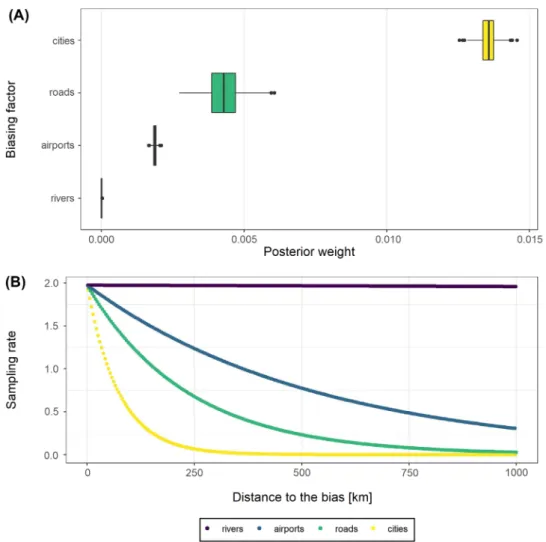
Figure 1. Results of the empirical validation analysis, estimating the accessibility bias in mammal occurrences from Borneo. (A) bias weights (w) defining the effects of each bias factor, (B) sampling rate as function of distance to the closest instance of each bias factor (the expected number of occurrences) given the inferred sampbias model. At the study scale of 0.05 degrees (ca 5 × 5 km) sampbias finds the strongest biasing effect for the proximity of cities and roads.

and summary method. Additional options exist to provide custom gazetteers, study area, spatial grid and grain size of the analysis, as well as operators for the calculation of the bias distances, including priors for q and w. A tuto-rial on how to use sampbias is available with the pack-age and in the electronic supplement of this publication (Supplementary material Appendix 1).

To exemplify the use of sampbias, we downloaded the occurrence records of all mammals available from the island of Borneo (n = 6262, GBIF.org 2016) and ran sampbias using the default gazetteers as shown in the example code (Box 1) below, to test the biasing effect of the main airports, cities and roads in the data set. The example data set is provided with sampbias.

We found a strong effect of cities on sampling intensity, a moderate effect of roads and airports and a negligible effect of rivers (Fig. 1). All models predict a low number of collec-tion records in the centre of Borneo (Fig. 2), which reflects the original data, and where accessibility means are low (Supplementary material Appendix 2 Fig. 1). The empirical example illustrates the use of sampbias, for detailed analyses or a smaller geographic scale, higher resolution gazetteers, including smaller roads and rivers and a higher spatial resolu-tion would be desirable. Results might change with increas-ing resolution, since roads and rivers might have a stronger effect on higher resolutions (facilitating most the access to their immediate vicinity), whereas cities and airports might have a stronger effect on the larger scale (facilitating access to a larger area).

We ran a simulation experiment to assess whether the esti-mated bias weights differ significantly from a null expectation of random sampling. To do so, we first simulated ten unbiased data sets by generating 6262 random occurrences across Borneo (the same number as in the empirical data set) and then ran sampbias with the same settings as for the empirical data set on each of these replicates. We found that the estimated bias parameters were significantly different (credible intervals non-overlapping) from the null model for cities, roads and airports (Supplementary material Appendix 2 Fig. 2).

sampbias is designed to work with sparsely sampled data sets. To test the performance of sampbias on small data sets we ran an additional simulation experiment. We ran sampbias with the same settings as for the empirical data set on three rarefied data sets, sub-sampling the initial data set to 3131,

Figure 2. Spatial projection of the sampling bias in an empirical example data set of mammal occurrences on the island of Borneo (down-loaded from <www.gbif.org>. GBIF.org 2016). The colours show the projection of the log10-transformed sampling rates (i.e. expected number of occurrences per cell) given the inferred sampbias model. The highest undersampling is in the centre of the island. Different visualizations, including among others the untransformed sampling rate are also implemented in sampbias.

626, 62 records respectively (three replicates each, a total of nine analyses), and then compared the estimated bias weights for all bias factors to the estimates for the empirical data set. The results showed that parameter estimates and the projec-tion of the bias effect in space were robust to the decreasing amount of data, although uncertainty increased as reflected larger estimated credible intervals (Supplementary material Appendix 2 Fig. 3–4).

Data accessibility

sampbias is available under a GNU General Public license v3 from <https://github.com/azizka/sampbias>, and includes the example data set as well as a tutorial (Supplementary material Appendix 1) and a summary of possible warnings produced by the package (Supplementary material Appendix 3).

Acknowledgements – We thank the organizers of the 2016 Ebben

Nielsen challenge for inspiring and recognizing this research. We thank all data collectors and contributors to GBIF for their effort. AZ is thankful for funding by iDiv via the German Research Foundation (DFG FZT 118), specifically through sDiv, the Synthesis Centre of iDiv. AA is supported by grants from the Swedish Research Council, the Knut and Alice Wallenberg Foundation, the Swedish Foundation for Strategic Research and the Royal Botanic Gardens, Kew. DS received funding from the Swiss National Science Foundation (PCEFP3_187012; FN-1749) and from the Swedish Research Council (VR: 2019-04739). Open access funding enabled and organized by Projekt DEAL.

Author contributions – All authors conceived this study, AZ and DS

developed the statistical algorithm and wrote the R-package, AZ and DS wrote the manuscript with contributions from AA.

References

Aiello-Lammens, M. E. et al. 2015. spThin: an R package for spa-tial thinning of species occurrence records for use in ecological niche models. – Ecography 38: 541–545.

Bache, S. M. and Wickham, H. 2014. magrittr: a forward-pipe operator for R. – <https://cran.r-project.org/web/packages/ magrittr/index.html>.

Barbosa, A. M. et al. 2013. Species-people correlations and the need to account for survey effort in biodiversity analyses. – Divers. Distrib. 19: 1188–1197.

Beck, J. et al. 2014. Spatial bias in the GBIF database and its effect on modeling species’ geographic distributions. – Ecol. Inform. 19: 10–15.

Bivand, R. S. et al. 2013. Applied spatial data analysis with R, 2nd edn. – Springer.

Boakes, E. H. et al. 2010. Distorted views of biodiversity: spatial and temporal bias in species occurrence data. – PLoS Biol. 8: e1000385. Boria, R. A. et al. 2014. Spatial filtering to reduce sampling bias

can improve the performance of ecological niche models. – Ecol. Model. 275: 73–77.

Botts, E. A.  et  al. 2011. Geographic sampling bias in the South African Frog Atlas Project: implications for conservation plan-ning. – Biodivers. Conserv. 20: 119–139.

Bystriakova, N. et al. 2012. Sampling bias in geographic and envi-ronmental space and its effect on the predictive power of species distribution models. – Syst. Biodivers. 10: 305–315.

Daru, B. H.  et  al. 2018. Widespread sampling biases in herbaria revealed from large-scale digitization. – New Phytol. 217: 939–955. Engemann, K.  et  al. 2015. Limited sampling hampers ‘big data’

estimation of species richness in a tropical biodiversity hotspot. – Ecol. Evol. 5: 807–820.

Fernández, D. and Nakamura, M. 2015. Estimation of spatial sam-pling effort based on presence-only data and accessibility. – Ecol. Model. 299: 147–155.

Fithian, W. et al. 2015. Bias correction in species distribution mod-els: pooling survey and collection data for multiple species. – Methods Ecol. Evol. 6: 424–438.

Fourcade, Y. et al. 2014. Mapping species distributions with MAX-ENT using a geographically biased sample of presence data: a performance assessment of methods for correcting sampling bias. – PLoS One 9: e97122.

Garnier, S. 2018. viridis: default color maps from ‘matplotlib’. – <https://cran.r-project.org/web/packages/viridis/index.html>. GBIF.org 2016. GBIF occurrence download, doi: 10.15468/dl.7fg4zx. Hijmans, R. J. 2019. geosphere: spherical trigonometry. – <https://

cran.r-project.org/web/packages/geosphere/index.html>. Isaac, N. J. B. and Pocock, M. J. O. 2015. Bias and information

in biological records. – Biol. J. Linn. Soc. 115: 522–531. Kadmon, R. et al. 2004. Effect of roadside bias on the accuracy of

predictive maps produced by bioclimatic models. – Ecol. Appl. 14: 401–413.

Kery, M. and Royle, J. A. 2016. Applied hierarchical modeling in ecology – analysis of distribution, abundance and species rich-ness in R and BUGS: Volume 1: Prelude and static models. – Academic Press, Elsevier.

Komori, O. et al. 2020. Sampling bias correction in species distri-bution models by quasi-linear Poisson point process. – Ecol. Inform. 55: 101015.

Kramer-Schadt, S.  et  al. 2013. The importance of correcting for sampling bias in MaxEnt species distribution models. – Divers. Distrib. 19: 1366–1379.

Lin, Y.-P. et al. 2015. Uncertainty analysis of crowd-sourced and professionally collected field data used in species distribution models of Taiwanese moths. – Biol. Conserv. 181: 102–110. Lobo, J. M. and Tognelli, M. F. 2011. Exploring the effects of

quantity and location of pseudo-absences and sampling biases on the performance of distribution models with limited point occurrence data. – J. Nat. Conserv. 19: 1–7.

Meyer, C. et al. 2015. Global priorities for an effective information basis of biodiversity distributions. – Nat. Commun. 6: 8221. Meyer, C. et al. 2016. Multidimensional biases, gaps and

uncertain-ties in global plant occurrence information. – Ecol. Lett. 19: 992–1006.

Monsarrat, S. et al. 2019. Accessibility maps as a tool to predict sampling bias in historical biodiversity occurrence records. – Ecography 42: 125–136.

Pebesma, E. J. and Bivand, R. S. 2005. Classes and methods for spatial data: the sp package. – R News 5: 21–41.

Phillips, S. J. et al. 2009. Sample selection bias and presence-only distribution models: implications for background and pseudo-absence. – Ecol. Appl. 19: 181–197.

Ruete, A. 2015. Displaying bias in sampling effort of data accessed from biodiversity databases using ignorance maps. – Biodivers. Data J. 3: e5361.

Rydén, O. et al. 2020. Linking democracy and biodiversity conserva-tion: empirical evidence and research gaps. – Ambio 49: 419–433. Shimadzu, H. and Darnell, R. 2015. Attenuation of species

abundance distributions by sampling. – R. Soc. Open Sci. 2: 140219.

Stolar, J. and Nielsen, S. E. 2015. Accounting for spatially biased sampling effort in presence-only species distribution modelling. – Divers. Distrib. 21: 595–608.

Vale, M. M. and Jenkins, C. N. 2012. Across-taxa incongruence in patterns of collecting bias. – J. Biogeogr. 39: 1744–1744. Varela, S.  et  al. 2014. Environmental filters reduce the effects of

sampling bias and improve predictions of ecological niche mod-els. – Ecography 37: 1084–1091.

Wickham, H. 2009. ggplot2 – elegant graphics for data analysis. – Springer.

Wickham, H. 2019. forcats: tools for working with categorical variables (factors). – <https://cran.r-project.org/web/packages/ forcats/index.html>.

Wickham, H. and Henry, L. 2019. tidyr: tidy messy data. – <https://cran.r-project.org/web/packages/tidyr/index.html>. Wickham, H.  et  al. 2019. dplyr: a grammar of data manipulation.

– <https://cran.r-project.org/web/packages/dplyr/index.html>. Yang, W. et al. 2013. Geographical sampling bias in a large

distri-butional database and its effects on species richness–environ-ment models. – J. Biogeogr. 40: 1415–1426.

Yang, W. et al. 2014. Environmental and socio-economic factors shaping the geography of floristic collections in China. – Global Ecol. Biogeogr. 23: 1284–1292.

Zizka, A. et al. 2020. Exploring the impact of political regimes on biodiversity. – VDem Working Papers 98: 1–13.

Supplementary material (available online as Appendix ecog-05102 at <www.ecography.org/appendix/ecog-ecog-05102>). Appendix 1–3.