Classifying tracked objects in far-field video surveillance

Classifying Tracked Objects in Far-Field Video

Surveillance

by

Biswajit Bose

B. Tech. Electrical Engineering

Indian Institute of Technology, Delhi, 2002

Submitted to the

Department of Electrical Engineering and Computer Science

in partial fulfillment of the requirements for the degree of

Master of Science in Electrical Engineering and Computer Science

at the

MASSACHUSETTS INSTITUTE OF TECHNOLOGY

February 2004

@

Mass

Author..

achusetts Institute of Technology 2004. All rights reserved.

MASSACHUSET7S INSTIWE OF TECHNOLOGY

APR 15

2004

....

...

... ... L

IB

R A R

IE S

Department of Electrical Engineering and Computer Science

January 8, 2004

C ertified by ...

... . ...

...

W. Eric L. Grimson

Bernard Gordon Professor of Medical Engineering

Thesis Supervisor

Accepted by...

Arthur C. Smith

Chairman, Department Committee on Graduate Students

Classifying Tracked Objects in Far-Field Video Surveillance

by

Biswajit Bose

Submitted to the Department of Electrical Engineering and Computer Science on January 8, 2004, in partial fulfillment of the

requirements for the degree of

Master of Science in Electrical Engineering and Computer Science

Abstract

Automated visual perception of the real world by computers requires classification of observed physical objects into semantically meaningful categories (such as 'car' or 'person'). We propose a partially-supervised learning framework for classification of moving objects-mostly vehicles and pedestrians-that are detected and tracked in a variety of far-field video sequences, captured by a static, uncalibrated camera. We introduce the use of scene-specific context features (such as image-position of objects) to improve classification performance in any given scene. At the same time, we design a scene-invariant object classifier, along with an algorithm to adapt this classifier to a new scene. Scene-specific context information is extracted through passive observation of unlabelled data. Experimental results are demonstrated in the context of outdoor visual surveillance of a wide variety of scenes.

Thesis Supervisor: W. Eric L. Grimson

Acknowledgments

I would like to thank Eric Grimson for his patient guidance and direction through these past 18 months, and for the freedom he has allowed me at the same time in my

choice of research topic.

People in the MIT Al Lab (CSAIL?) Vision Research Group have helped create a very friendly work environment. Thanks Gerald, Mario, Chris, Neal, Kevin, Mike, Kinh, ... the list goes on. In particular, without Gerald's help, I would have found navigating the strange world of computer programming much more painful. And Chris has always been very tolerant of my questions/demands regarding his tracking system.

The work described herein would not have been possible without the continued support provided by my father and mother, Tapan and Neera Bose.

Contents

1 Introduction 13

1.1 Object Classification . . . . 14

1.1.1 Object Classification Domains . . . . 15

1.1.2 Applications of Far-Field Object Classification . . . . 16

1.1.3 Challenging Problems in Far-Field Classification . . . . 17

1.2 Problem Statement . . . . 18

1.3 Outline of our Approach . . . . 19

1.4 Organisation of the Thesis . . . . 20

2 Far-Field Object Detection and Classification: A Review 21 2.1 Object Localisation in a Video Frame . . . . 21

2.2 Related Work: Object Classification . . . . 23

2.2.1 Supervised Learning . . . . 23

2.2.2 Role of Context in Classification . . . . 24

2.3 Related Work: Partially Supervised Learning . . . . 25

2.4 Where This Thesis Fits In . . . . 25

3 Steps in Far-field Video Processing 27 3.1 Background Subtraction . . . . 27

3.2 Region Tracking . . . . 28

3.3 Object Classification . . . . 29

3.3.1 F iltering . . . . 29

3.3.3 _{Classifier Architecture . . . .}

3.3.4 _{Classification with Support Vector Machines . . . .} 3.4 Activity Understanding using Objects . . . .

4 Informative Features for Classification

4.1 Features for Representing Objects . . . . 4.2 Moment-Based Silhouette Representation . . . . 4.2.1 Advantage of Moment-Based Representations . . 4.2.2 Additional Object Features . . . . 4.3 _{Using Mutual Information Estimates for Feature Selection} 4.4 Feature Selection for a Single Scene . . . .

4.4.1 Information Content of Individual Features . . . . 4.4.2 Information Content of Feature Pairs . . . . 4.4.3 Context Features . . . . 4.5 Feature Grouping for Multiple Scenes . . . . 5 Transferring Classifiers across Scenes

5.1 Scene Transfer . . . . 5.2 _{Scene Adaptation . . . .} 6 Experimental Results

6.1 Selection of Experimental Data . . . . 6.2 Classification Performance . . . . 6.3 Performance Analysis . . . . 6.3.1 Role of Position as a Context Feature . . . . 6.3.2 Choice of Thresholds for Feature Selection and Grouping . . . 6.3.3 Failure Cases . . . . 7 Conclusion and Discussion

32 34 36 37 . . . . . 37 . . . . . 38 . . . . . 39 . . . . . 40 . . . . . 42 . . . . . 44 . . . . . 44 . . . . . 47 . . . . . 49 . . . . . 51 55 55 56 59 59 60 63 63 64 64 65

List of Figures

1-1 Examples of far-field scenes. . . . . 17

3-1 An illustration of background subtraction: (a) a video frame, (b) current background model, and (c) pixels identified as belonging to the foreground (shown against a light-grey background for clarity). Note the parked car in (b), which is considered part of the background, and the shadow of the moving car in (c), which is detected as foreground. . . . . 28

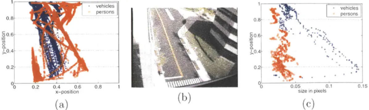
4-1 (a) Scatter plot illustrating spatial distribution of vehicles and persons in scene (a) of Figure 1-1 (which is shown again here in (b) for convenience), in which significant projective foreshortening is evident. (c) Using the y-coordinate as a normalising feature for bounding-box size can greatly im-prove performance, as demonstrated by the fact that vehicles and

pedestri-ans are clearly distinguishable in the 2D feature space. . . . . 50

List of Tables

3.1 _{List of object features considered. (bg. =background, fg.=foreground,}

deriv. =derivative, norm. =normalised.) Definitions and expressions for

features are given in Section 4.2. . . . . 31

4.1 Exhaustive set of features for representing object silhouettes. . . . . . 41

4.2 Average mutual information (M.I.) scores between object features and

labels in a single scene (averaged over seven scenes), along with decision to select (y) or reject (n) features. M.I. is measured in bits (maximum possible score = 1.0). (p) means the decision was made after consider-ing M.I. scores for pairs of features. bg.=background, fg.=foreground,

deriv. =derivative, norm. =normalised. . . . . 45

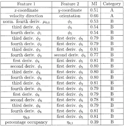
4.3 Mutual information (MI) scores of note between pairs of object

fea-tures and labels in a single scene, along with corresponding decision to select both the features (A) or reject the first feature (B) in the pair. MI scores are given in bits. See Section 4.4.2 for an explanation of

categories A and B. . . . . 46

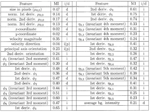
4.4 Mutual information (M.I.) scores between object features and labels across multiple scenes, along with decision regarding whether feature is scene-dependent (d) or scene-independent (i). M.I. is measured in

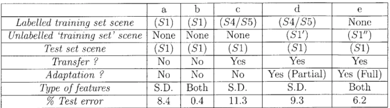
6.1 Performance evaluation for scene Si (Figure 6-1): test errors using var-ious classifiers and features. 'S.D.' = scene-dependent features. 'Both' = scene-dependent + scene-independent features. Labels for Si' are produced in step c, and those for Si" in step d. . . . . 62

Chapter 1

Introduction

Computer vision (or machine vision) is currently an active area of research, with the goal of developing visual sensing and processing algorithms and hardware that can see and understand the world around them. A central theme in computer vision is the description of an image (or video sequence) in terms of the meaningful objects that comprise it (such as persons, tables, chairs, books, cars, buildings and so on). While the concept of an 'object' comes rather naturally to humans (perhaps because of our constant physical interaction with them), it is very difficult for a computer programme to identify distinct objects in the image of a scene (that is, to tell which pixels in the image correspond to which object). This problem of detection or segmentation is an active area of research. Segmentation of a bag of image pixels into meaningful object regions probably requires an intelligent combination of multiple visual cues: colour, shape (as defined by a silhouette), local features (internal edges and corners), spatial continuity and so on. The problem is made challenging by the facts that computers, unlike people, have no a priori knowledge of the orientation and zoom of the sensing device (i.e., the camera) and objects are often only partially visible, due to occlusion by other objects which are in the line of sight. Nevertheless, human performance illustrates that these problems are solvable, since they themselves can identify objects in random images shown to them.

Shifting focus from images to video sequences might seem to make matters worse for computer programmes, since this adds an extra temporal dimension to the data.

However, video provides added information that simplifies object detection in that motion in the scene can be used as a cue for separating moving foreground objects from a static background. Object motion can also be used as a feature for distinguishing between different object classes. Further, by tracking objects in video across multiple frames, more information can be obtained about an object's identity.

As the main application of our research is to activity analysis in a scene, we restrict our attention in this thesis to video sequences captured by static cameras and seek to detect and classify objects that move (such as vehicles and pedestrians) in the scene.

1.1

Object Classification

Given a candidate image region in which an object might be present, the goal of object classification is to associate the correct object class label with the region of interest. Object class labels are typically chosen in a semantically meaningful manner, such as 'vehicle', 'pedestrian', 'bird' or 'airplane'. Humans can easily understand events happening around them in terms of interactions between objects. For a computer to reach a similar level of understanding about real-world events, object classification is an important step.

Detection of moving objects in the scene is just the first step towards activity analysis. The output of a motion-based detector is essentially a collection of fore-ground regions (in every frame of a video sequence) that might correspond to moving objects. Thus, the detection step acts as a filter that focuses our attention on only certain regions of an image. Classification of these regions into different categories of objects is still a huge challenge.

Object classification is often posed as a pattern recognition problem in a super-vised learning framework [12]. Under this framework, probabilistic models are used for describing the set of features of each of the N possible object classes, and the

class label assigned to a newly detected foreground region corresponds to the ob-ject class that was most likely to have produced the set of observed features. Many different object representations (i.e. sets of features) have been proposed for the

purpose of classification, including 3D models, constellation of parts with character-istic local features, raw pixel values, wavelet-based features and silhouette shape (for example,

[15,

13, 31, 32]). However, no one representation has been shown to be uni-versally successful. This is mainly because of the wide range of conditions (including varying position, orientation, scale and illumination) under which an object may need to be classified.

For our purposes, object classification is a process that takes a set of observations of objects (represented using suitable features) as input, and produces as output the probabilities of belonging to different object classes. We require the output to be a probability score instead of a hard decision since this knowledge can be useful for further processing (such as determining when to alert the operator while searching for anomalous activities).

As a supervised learning problem, the time complexity of training for most clas-sification algorithms is quadratic in the number of labelled examples, because of the need to calculate pairwise inner- and/or outer-products in the given feature space. Time complexity for testing is linear in the number of inputs (and perhaps also in the number of training examples). Classifier training is typically performed offline, while testing may be performed either online or offline.

1.1.1

Object Classification Domains

Many visual processes, including object classification, can be approached differently depending on the domain of application: near-, mid- or far-field. These domains are distinguished based on the resolution at which objects are imaged, as this decides the type of processing that can be performed on these objects. In the near-field domain, objects are typically 300 pixels or more in linear dimension. Thus, object sub-parts (such as wheels of a car, parts of a body, or features on a face) are clearly visible. In the far-field domain, objects are typically 10 to 100 pixels in linear dimension. In this situation, the object itself is not clearly visible, and no sub-parts can be detected. Anything in between these two domains can be considered mid-field processing (where the object as a whole is clearly visible, and some sub-parts of an object may be just

barely visible).

We address the task of object classification from far-field video. The far-field setting provides a useful test-bed for a number of computer vision algorithms, and is also of practical value. Many of the challenges of near-field vision-dealing with unknown position, orientation and scale of objects, under varying illumination and in the presence of shadows-are characteristics of field vision too. Automated far-field object classification is very useful for video surveillance, the objective of which is to monitor an environment and report information about relevant activity. Since activities of interest may occur infrequently, detecting them requires focused obser-vation over prolonged intervals of time. An intelligent activity analysis system can take much of this burden off the user (i.e. security personnel). Object classification

is often a first step in activity analysis, as illustrated in Section 1.1.2.

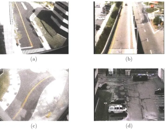
In far-field settings, a static or pan-tilt surveillance camera is typically mounted well away from (and typically at some elevation above) the region of interest, such that projected images of objects under surveillance (such as persons and vehicles) range from 10 to 100 pixels in height. Some sample far-field scenes are shown in Figure 1-1.

1.1.2

Applications of Far-Field Object Classification

Far-field object classification is a widely studied problem in the video surveillance research community, since tasks such as automatic pedestrian detection or vehicle de-tection are useful for activity analysis in a scene [20, 29, 38]. A single round-the-clock far-field surveillance camera, installed near an office complex, car-park or airport, may monitor the activities of thousands of objects-mostly vehicles and persons-every day. In a surveillance system comprising multiple cameras, simply providing the raw video data to security personnel can lead to information overload. It is thus very useful to be able to filter events automatically and provide information about scene activity to a human operator in a structured manner. Classification of moving objects into predefined categories allows the operator to programme the system by specifying events of interest such as 'send alert message if a person enters building A

(a) (b)

(c) (d)

Figure 1-1: Examples of far-field scenes.

from area B,' or 'track any vehicles leaving area C after 3 p.m.' Classification also provides statistical information about the scene, to answer questions such as finding 'the three most frequent paths followed by vehicles when they leave parking garage D' or 'the number of persons entering building E between 8 a.m. and 11 a.m.'.

1.1.3

Challenging Problems in Far-Field Classification

The far-field domain is particularly challenging because of the low resolution of ac-quired imagery: objects are generally less than 100 pixels in height, and may be as small as 50 pixels in size. Under these conditions, local intensity-based features (such as body-parts of humans) cannot be reliably extracted. Further, as many far-field cameras are set up to cover large areas, extracted object features may show signif-icant projective distortion-nearby objects appear to be larger in size and to move faster than objects far away.

restricted settings for which they have been built or trained, but can also fail

spec-tacularly when transferred to novel environments. Sometimes, the scene-specificity is explicitly built into the system in the form of camera calibration. Lack of invariance of the existing methods to some scene-dependent parameter, such as position, orienta-tion, illuminaorienta-tion, scale or visibility, is often the limiting factor preventing widespread use of vision systems. This is in stark contrast to the human visual system, which works reasonably well even under dramatic changes in environment (e.g. changing

from far-field to near-field). What is missing in automated systems is the ability to

adapt to changing or novel environments.

Our goal in the present work is to overcome the challenge of limited applicability of far-field classification systems. This is made explicit in the problem statement given in the next section.

1.2

Problem Statement

Given a number of video sequences captured by static uncalibrated cameras in differ-ent far-field settings (at least some of which are a few hours in duration and contain more than 500 objects), our objectives are:

" To demonstrate a basic object classification system (that uses the output of Inotion-based detection and tracking steps) based on supervised learning with a small number of labelled examples, to distinguish between vehicles, pedestrians and clutter with reasonably high accuracy.

" To propose a systematic method for selecting object features to be used for classification, so as to achieve high classification performance in any given scene, but also be able to classify objects in a new scene without requiring further supervised training.

o To propose an algorithm for transferring object-classifiers across scenes, and subsequently adapting them to scene-specific characteristics to minimise classi-fication error in any new scene.

1.3

Outline of our Approach

Our work is based on an existing object-detection and tracking system that employs adaptive background subtraction

[35].

The regions of motion detected by the tracking system are fed as input to our classification system. After a filtering step in which most meaningless candidate regions are removed (such as regions corresponding to lighting change or clutter), our system performs two-class discrimination: vehicles vs. pedestrians. We restrict our attention to these two classes of objects since they occur most frequently in surveillance video. However, our approach can be generalised to hierarchical multiclass classification.

Our goal is to address the conflicting requirements of achieving high classifica-tion performance in any single scene but also being able to transfer classifiers across scenes without manual supervision. We aim to do this without any knowledge of the position, orientation or scale of the objects of interest. To achieve the first goal, we introduce the use of scene-specific local context features (such as image-position of an object or the appearance of the background region occluded by it). We also identify some other commonly used features (such as object size) as context features. These context features can easily be learnt from labelled examples. However, in order to be consistent with our second goal, we use only scene-invariant features to design a baseline classifier, and adapt this classifier to any specific scene by learning context features with the help of unlabelled data. While learning from unlabelled data is a well-studied problem, most methods assume the distributions of labelled and un-labelled data are the same. This is not so in our case, since context features have different distributions in different scenes. Thus, we propose a new algorithm for incor-porating features with scene-specific distributions into our classifier using unlabelled data.

We make three key contributions to object classification in far-field video se-quences. The first is the choice of suitable features for far-field object classification from a single, static, uncalibrated camera and the design of a principled technique for classifying objects of interest (vehicles and pedestrians in our case). The second

is the introduction of local, scene-specific context features for improving classification performance in arbitrary far-field scenes. The third is a composite learning algorithm that not only produces a scene-invariant baseline classifier that can be transferred across scenes, but also adapts this classifier to a specific scene (using context fea-tures) by passive observation of unlabelled data.

Results illustrating these contributions are provided for a wide range of far-field scenes, with varying types of object paths, object populations and camera orientation and zoom factors.

1.4

Organisation of the Thesis

Chapter 2 gives an overview of the problem of object detection and classification in far-field video, and a review of previous work done in this area. The basic moving object detection and tracking infrastructure for far-field video on which our object classification system is built is described in Chapter 3. Our choice of features, as well as the feature selection and grouping process, resulting in the separation of features into two categories-scene-dependent and scene-independent-is discussed in Chapter 4. Chapter 5 presents our algorithm for developing a baseline object classifier (which can be transferred to other scenes) and adapting it to new scenes. Experimental results and analysis are presented in Chapter 6. Chapter 7 summarises the contributions of our work and mentions possible applications, as well as future directions for research.

Chapter 2

Far-Field Object Detection and

Classification: A Review

This chapter presents an overview of various approaches to object classification in far-field video sequences. We start by analysing the related problems of object detection and object classification, and then go on to review previous work in the areas of far-field object classification and partially-supervised classification.

2.1

Object Localisation in a Video Frame

To define an object, a candidate set of pixels (that might correspond to an object) needs to be identified in the image. Two complementary approaches are commonly used for localisation of candidate objects. These two approaches can be called the motion-based approach and the object-specific (image-based) approach.

Classification systems employing the motion-based approach assume a static cam-era and background, and use background subtraction, frame-differencing or optical flow to detect moving regions in each video frame [14, 20, 25]. Detected regions are then tracked over time, and an object classification algorithm is applied to the tracked regions to categorise them as people, groups of people, cars, trucks, clutter and so on. The key feature of this approach is that the detection process needs very little knowledge (if any) of the types of objects in the scene. Instead, the burden of

categorising a detected motion-region as belonging to a particular object class is left to a separate classification algorithm. Common features for classifying objects after motion-based detection include size, aspect ratio and simple descriptors of shape or motion.

The other popular approach, direct image-based detection of specific object classes, does not rely on object tracking. Instead, each image (or video-frame) is scanned in its entirety, in search of regions which have the characteristic appearance of an ob-ject class of interest, such as vehicles [23, 24] or pedestrians

[27].

The class-specific appearance models are typically trained on a number of labelled examples of ob-jects belonging to that class. These methods typically use combinations of low-level

features such as edges, wavelets, or rectangular filter responses.

The main advantage of motion-based detection systems is that they serve to focus the attention of the classification system on regions of the image (or video-frame) where objects of interest might occur. This reduces the classification problem from discriminating between an object and everything else in the frame (other objects and the background) to only discriminating between objects (belonging to known or even unknown classes). As a result, false detections in background regions having an appearance similar to objects of interest are avoided. Motion-based detection methods can thus lead to improved performance if the number of objects per frame (and the area occupied by them) is relatively small. Detection of regions of motion also automatically provides information about the projected orientation and scale of the objects in the image (assuming the entire object is detected to be in motion, and none of the background regions are detected as foreground).

A disadvantage of object detection methods based on background-subtraction is that they cannot be used if the motion of the camera is unknown or arbitrary. Also, background-subtraction cannot be used for detecting objects in a single image. However, this is not a severe limitation in most situations, because objects of interest will probably move at some point in time (and can be monitored and maintained even while static) and video for long-term analysis of data has to be captured by a static or pan-tilt-zoom camera.

Other disadvantages of background subtraction (relative to image-based detection) include its inability to distinguish moving objects from their shadows, and to separate objects whose projected images overlap each other (e.g. images of vehicles in dense, slow-moving traffic). A combination of image-based and motion-based detection (as in [38], for example) will probably work better than either of the two methods in isolation.

2.2

Related Work: Object Classification

Much work has been done recently on far-field object classification in images and video sequences. In this section, we provide an overview of classification techniques for both object specific (image-based) and motion-based detection systems.

2.2.1

Supervised Learning

Object classification can be framed as a supervised learning problem, in which a learn-ing algorithm is presented with a number of labelled positive and negative examples during a training stage. The learning algorithm (or classifier) estimates a decision boundary that is likely to provide lowest possible classification error for unlabelled test examples drawn from the same distribution as the training examples. Use of a learning algorithm thus avoids having to manually specify thresholds on features for deciding whether or not a given object belongs to a particular class.

Various types of learning algorithms have been used for object classification prob-lems. A simple yet effective classifier is based on modelling class-conditional probabil-ity densities as multivariate gaussians [22, 25]. Other types of classification algorithms include support vector machines [27, 28, 31], boosting [24, 38], nearest-neighbour clas-sifiers, logistic linear classifiers [10], neural networks [17] and Bayesian classification using mixtures of gaussians.

Another important decision affecting classification performance is the choice of features used for representing objects. Many possible features exist, including entire images [11, 31], wavelet/rectangular filter outputs [28, 38], shape and size [20, 25],

morphological features [14], recurrent motion [9, 20] and spatial moments [17].

Labelled training examples are typically tedious to obtain, and are thus often available only in small quantities. Object-specific image-based detection methods re-quire training on large labelled datasets, especially for low-resolution far-field images. Most detection-based methods have severe problems with false positives, since even a false-positive rate as low as 1 in 50,000 can produce one false positive every frame. To get around this problem, Viola et al. [38] have recently proposed a pedestrian detec-tion system that works on pairs of images and combines appearance and modetec-tion cues. To achieve desired results, they use 4500 labelled training examples for detecting a single class of objects, and manually fix the scale to be used for detecting pedestrians. Methods based on background subtraction followed by object tracking suffer much less from the problems of false positives or scale selection, and have been demonstrated to run in real-time [35]. These methods may also be able to track objects robustly in the presence of partial occlusion and clutter.

2.2.2

Role of Context in Classification

Use of contextual knowledge helps humans perform object classification even in com-plicated situations. For instance, humans can correctly classify occluded objects when these are surrounded by similar objects (such as a person in a crowd) and have no trouble distinguishing a toy-car from a real one, even though they look alike. In many situations, prior knowledge about scene characteristics can greatly help automated interpretation tasks such as object classification and activity analysis. Contextual information (such as approximate scale or likely positions of occurrence of objects) may be manually specified by an operator for a given scene, to help detect certain

activities of interest. [6, 26].

Torralba and Sinha [37] have shown that global context can be learnt from ex-amples and used to prime object detection. They propose a probabilistic framework for modelling the relationship between context and object properties, representing global context in terms of the spatial layout of spectral components. They use this framework to demonstrate context driven focus of attention and scale-selection in real

world scenes.

2.3

Related Work: Partially Supervised Learning

Obtaining labelled training data for object classifiers is not easy, especially if hun-dreds of examples are needed for good performance. Methods based on exploiting unlabelled data provide a useful alternative. Many of these were originally developed in the machine learning community for text classification problems [4, 21], and have recently been applied to object detection/classification problems in the machine vision community. Levin et al. [24] use a co-training algorithm [4] to help improve vehicle detection using unlabelled data. This algorithm requires the use of two classifiers that work on independent features, an assumption that is hard to satisfy in practice. Wu and Huang

[39]

propose a new algorithm for partially supervised learning in the context of hand posture recognition. Stauffer [34] makes use of multiple observations of a single object (obtained from tracking data) to propagate labels from labelled examples to the surrounding unlabelled data in the classifier's feature space.

2.4

Where This Thesis Fits In

The problem of developing classifiers which will work well across scenes has not been directly addressed in the machine vision community. Existing systems tend to make scene-specific assumptions to achieve high performance. Our aim is to be able to classify objects across a wide range of positions, orientations and scales.

To the best of our knowledge, no previous work has been done on learning local context features (such as position and direction of motion of objects) from long-term observation, to improve object classification in scenes observed by a static camera.

Our problem also differs from most of the well-studied problems in the machine learning community because a sub-set of the object features that we consider-the scene-specific context features-have different distributions in different scenes. We propose to identify these scene-specific features and initially keep them aside. Later,

after training a classifier using the remaining features, the information contained in the scene-specific features is gradually incorporated by retraining with the help of confidence-rated unlabelled data.

A method for solving a problem that is very similar at the abstract level-combining features whose distribution is the same across data sets with other features whose distribution is data set dependent-has been proposed in

[3].

Our approach differs from theirs in the classification algorithm used, as well as in our use of mutual information estimates to perform feature selection and grouping.

Chapter 3

Steps in Far-field Video Processing

This chapter presents the basic infrastructure and processing steps needed in going

from raw video to object classification and activity analysis. While the emphasis is on the components of the object classification architecture, necessary details of other processing steps such as background subtraction and region-tracking are given. Defi-nitions of important terms and descriptions of standard algorithms are also provided.

3.1

Background Subtraction

Throughout our work, we rely on distinguishing objects of interest from the back-ground in a video sequence based on the fact that the former move at some point in time (though not necessarily in every frame). Given that a particular scene has been observed for long enough by a static camera, and that an object of interest moves by a certain minimum amount, background subtraction is a relatively reliable method for detecting the object.

Background subtraction consists of two steps: maintaining a model of the back-ground, and subtracting the current frame from this background model to obtain the

current foreground. A simple yet robust background model is given by calculating the

Inedian intensity value at each pixel over a window of frames. More complex models can adapt to changing backgrounds by modelling the intensity distribution at each pixel as a gaussian (or mixture of gaussians) and updating the model parameters in

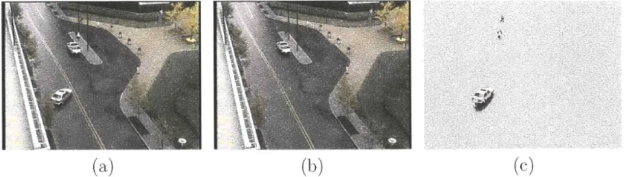
(a) (b) (c)

Figure 3-1: An illustration of background subtraction: (a) a video frame, (b) current background model, and (c) pixels identified as belonging to the foreground (shown against a light-grey background for clarity). Note the parked car in (b), which is considered part of the background, and the shadow of the moving car in (c), which is detected as foreground.

an online manner [35]. Adaptive backgrounding is useful for long-term visual surveil-lance, since lighting conditions can change with time, and vehicles might be parked

in the scene (thus changing from foreground to background).

The output of the background subtraction process is a set of foreground pixels, as illustrated in Figure 3-1. At this stage, there is not yet any concept of an object. By applying spatial continuity constraints, connected component regions can be identified as candidate objects. We call each connected-component in a frame a motion-region (or an observation). The information stored for an observation include the centroid location in the frame, the time of observation and the pixel values (colour or grey-scale) for the foreground region within an upright rectangular bounding-box just enclosing the connected-component.

3.2

Region Tracking

The motion-regions identified in each frame by background subtraction need to be associated with one another (across time) so that multiple instances of the same object are available for further processing (such as classification). This is a classic problem of data association and tracking, which has been extensively studied for radar and sonar applications [2]. A simple data association technique uses spatial proximity

and similarity in size to assign motion-regions in the current frame with those in the previous frame, while allowing for starting and stopping of tracking sequences if no

suitable match is found.

We define a tracking sequence (or a track) as a sequence of observations of (sup-posedly) the same object. The output of the tracking system consists of a set of object tracks. The individual observations that constitute a track are also called instances of a track.

The advantage of performing tracking after background subtraction is that the number of candidate regions for the inter-frame data association problem is greatly reduced. At the same time, many false positives-regions where motion was detected even though there was no moving object present-are eliminated by preserving only those tracks which exceed a certain minimum number of frames in length.

For the purposes of this thesis, background subtraction and tracking were treated as pre-processing steps, and an existing implementation of these steps (developed by Chris Stauffer [35]) was used. We now discuss our main contribution: development of a far-field object classification system.

3.3

Object Classification

Many image-based detection systems implicitly perform classification at the same time as detection, as discussed in Section 2.2. Recently, a few systems have been proposed to use background-subtraction for object detection. In such systems, object classification is a treated as a pattern classification step, involving use of a suitable classification algorithm that is run on the detected and tracked motion-regions with an appropriate set of features. Our system falls into this category.

Pattern classification is a well-studied problem in the field of statistical learning. In this section, we discuss our formulation of object classification from tracking sequences as a supervised pattern classification problem.

3.3.1

Filtering

To demonstrate our algorithms for scene-transfer and scene-adaptation, we consider classification of vehicles and pedestrians. As a pre-processing step, we automatically

filter the tracking data to remove irrelevant clutter, thus reducing the classification task to a binary decision problem. Filtering is an important step for long-term surveil-lance, since (random sampling shows that) more than 80% of detected moving regions are actually spurious objects. This is mainly because lighting changes take place con-tinually and trees are constantly swaying in the wind. Features useful for filtering include minimum and maximum size of foreground region (to filter abrupt changes in lighting), minimum duration (to filter swaying trees), minimum distance moved (to filter shaking trees and fluttering flags) and temporal continuity (since apparent size and position of objects should change smoothly).

Even after filtering out clutter, there are certain classes of objects that are neither vehicles nor pedestrians, such as groups of people and bicycles. Including these classes in the analysis is left for future work.

3.3.2

Video Features

As of December 2003, no single set of visual features has been shown to work for generic object classification or recognition tasks. The choice of features is thus often task-dependent.

There are some common intuitive guidelines, such as use of appearance based features to distinguish objects: a face has a very different appearance from a chair or desk. However, in far-field situations, very few pixels are obtained per object, so local appearance-based features such as parts of a face or body parts of a person cannot be reliably detected. Low resolution data in far-field video prevent us from reliably detecting parts-based features of objects using edge- and corner-descriptors. Instead, we use spatial moment-based features (and their time derivatives) that provide a global description of the projected image of the object, such as size of object silhouette and orientation of its principal axis. The full list of object features we consider is given in Table 3.1; definitions for these features are provided in Section 4.2. Speed, direction of motion and other time derivatives are motion-based features that cannot be used for object classification from a single image.

Feature Feature size in pixels (po,o) 1st deriv. 6

norm. 1st deriv. po,o 2nd deriv. 6

norm. 2nd deriv. pio,o 3rd deriv. #6

norm. 3rd deriv. p0,0 4th deriv. 06 norm. 4th deriv. po,o

'q4,0 (invariant 4th moment)

x-coordinate 'q3,1 (invariant 4th moment)

y-coordinate 72,2 (invariant 4th moment)

velocity magnitude '11,3 _{(invariant 4th moment)}

velocity direction T/0,4 (invariant 4th moment)

acceleration magnitude 1st deriv. 'q4,o

acceleration direction 2nd deriv. T14,0

1st deriv. 77₃,₁ principal axis orientation 2nd deriv. 773,1

1st deriv. orientation 1st deriv. 772,2

2nd deriv. orientation 2nd deriv. T/2,2

3rd deriv. orientation 1st deriv. r71,3

#1 (invariant 2nd moment) 2nd deriv. r11,3

#2 (invariant 2nd moment) 1st deriv. 70,4

1st deriv. #1 2nd deriv. 770,4

2nd deriv. 01 r75,o (invariant 5th moment) 3rd deriv. 01 74,1 (invariant 5th moment)

4th deriv. 01 73,2 (invariant 5th moment)

1st deriv. 02 72,3 (invariant 5th moment)

2nd deriv. #2 71,4 (invariant 5th moment)

3rd deriv. #2 770,5 _{(invariant 5th moment)}

4th deriv. #2 1st deriv. 15,0 03 (invariant 3rd moment) 1st deriv. 74,1 #4 (invariant 3rd moment) 1st deriv. 73,2 #5 (invariant 3rd moment) 1st deriv. 72,3 #6 (invariant 3rd moment) 1st deriv. 71,4

1st deriv. 03 1st _{deriv. r7O,5} 2nd deriv. #3

3rd deriv. #3 percentage occupancy 4th deriv. 03 1st deriv. occupancy

1st deriv. 04 2nd deriv. occupancy 2nd deriv. 4

3rd deriv. #4 average bg. intensity 4th deriv. #4 average fg. intensity 1st deriv. 05 average bg. hue

2nd deriv. #s average fg. hue 3rd deriv. #s 1st deriv. fg. intensity 4th deriv. s 1st deriv. fg. hue Table 3.1: List of object features considered. (bg.=background, deriv. =derivative, norm.=nornalised.) Definitions and expressions given in Section 4.2.

fg.=foreground, for features are

using mutual information estimates. This is described in Chapter 4. Our reasons for choosing the features mentioned are also discussed there.

Video sequences provide us with two kinds of features, which we call instance features and temporal features. Instance features are those that can be associated with every instance of an object (that is, with each frame of a tracking sequence). The size of an object's silhouette and the position of its centroid are examples of instance features. Temporal features, on the other hand, are features that are associated with an entire track, and cannot be obtained from a single frame. For example, the mean aspect-ratio or the Fourier coefficients of image-size variation are temporal features. Temporal features can provide dynamical information about the object, and can generally only be used after having observed an entire track (or some extended portion thereof). However, temporal features can be converted into instance features by calculating them over a small window of frames in the neighbourhood of a given frame. For example, apparent velocity of the projected object is calculated in this way.

3.3.3

Classifier Architecture

Tracking sequences of objects can be classified in two ways: classifying individual instances in a track separately (using instance features) and combining the instance-labels to produce an object-label, or classifying entire object tracks using temporal features. We chose an instance classifier, for two reasons. Firstly, labelling a single object produces many labelled instances. This helps in learning a more reliable clas-sifier from a small set of labelled objects. Secondly, a single instance feature (e.g. position of an object in a frame) often provides more information about the object class than the corresponding temporal feature (e.g. mean position of an object).

Each detected object is represented by a sequence of observations, 0 {Oi}, 1

i < n, where n is the number of frames for which the object was tracked. Classifi-cation of this object as a vehicle or pedestrian can be posed as a binary hypothesis-testing problem, in which we choose the object class label l following the

maximum-likelihood (ML) rule [12]:

1* = argmax p(O I ) (3.1)

(i.e. choose ij corresponding to the higher class-conditional density p(OIl1)). We use

the ML rule instead of the maximum a posteriori (MAP) rule because we found the prior probabilities, p(lj), to be strongly scene-dependent. For instance, while some scenes contain only vehicles, some other contain three times as many pedestrians as vehicles. To develop a scene-invariant classifier, we assume p(li) = p(l2).

The likelihood-ratio test (obtained from Equation 3.1) involves evaluation of p(01, ..., On l1), the joint probability of all the observations conditioned on the class label. For images

of a real moving object, this joint distribution depends on many physical and geomet-ric factors such as object dynamics and imaging parameters. A simplifying Markov approximation would be to model the joint probability as a product of terms repre-senting conditional probabilities of each observation given only its recent neighbours in the sequence. However, we choose to avoid estimation of even these conditional probabilities, as their parameters vary with the position of the observation (due to projective distortion). Instead, we search for (approximately) independent observa-tions in the sequence, since the joint probability for independent samples is simply

n

given by p(OiIlj) (i.e., no additional probability distributions are needed to model

inter-observation dependences). For every i and j, the probability p(Oill) can in turn be obtained from the posterior probability of the label given the observation,

p(ljlOi), by applying Bayes' rule (and cancelling out the marginal observation

prob-abilities upon taking the likelihood ratio):

p(Oil(1) = . (3.2)

This means that our classifier can be run separately on each independent observation in a sequence, to produce the corresponding posterior probability of the class label. We approximate independent samples by looking for observations between which the imaged centroid of the object moves a minimum distance. This is useful, for example, to avoid using repeated samples from a stopped object (which is quite common for

both vehicles and persons in urban scenes). In our implementation, the minimum distance threshold is equal to the object-length.

3.3.4

Classification with Support Vector Machines

In choosing a suitable classifier, we considered using a generative model (such as a mixture of Gaussians), but decided against it to avoid estimating multi-dimensional densities from a small amount of labelled data. Instead, we chose a discriminative model-support vector machine (SVM) with soft margin and Gaussian kernel-as our instance classifier. (The use of a soft margin is necessary since the training data are non-separable.) In the SVM formulation (for nonseparable data), we look for the maximum-margin separating hyperplane (parameterised by w and b) for the N training points xi E Rk (in a k-dimensional feature space) and corresponding labels yj E

{-1,

1}, given the optimisation problem

[7]:

Minimise - W -W

+

7 i subject to (3.4) and > 0, (3.3) 2

where we have introduced N nonnegative variables = ( 1, 2, ... , -N) such that

yi(w -xi + b) ;> 1 - i, i = 1, 2, ..., N, (3.4)

to account for the fact that the data are nonseparable. As in the separable case, this can be transformed into the dual problem:

N N

Maximise E 2 E aeaajyiyyK(xi,

zz

xj) (3.5)

i=1 2i,j=l

subject to

where a, are the Lagrange multipliers (with associated upper-bound C) and K rep-resents the SVM kernel function. Applying the Kuhn-Tucker conditions, we get

ai(yi(K(w, xi) + b) - 1I + i) 0 (3.7)

(C - a2)i= 0 (3.8)

It is useful to distinguish between the support vectors for which ai < C and those for which ai = C. In the first case, from condition (3.8) it follows that i = 0, and hence, from condition (3.7), these support vector are margin vectors. On the other hand, support vectors for which ai = C are mostly either misclassified points, or correctly classified points within the margin. The bounds on the Lagrange multipliers help to provide a 'soft margin', whereby some examples can lie within the margin, or even on the wrong side of the classification boundary.

For training our baseline (scene-invariant) object classifier (Section 5.1), we fixed

C to a large value (= 1,000). Our scene-adaptation algorithm (Section 5.2), however, uses different values of C for different 'labelled' examples, depending on the confidence of the associated label.

One disadvantage of using SVMs is that the output, di, is simply the signed distance of the test instance from the separating hyperplane, and not the posterior probability of the instance belonging to an object class. Posterior probabilities are needed to correctly combine instance labels using the ML rule to obtain an object label. To get around this problem, we retrofit a logistic function g(d) that maps the SVM outputs di into probabilities [30]:

1

g (di) -1 + exp(-di) (3.9)

The posterior probability is then given by

where the parameter A is chosen such as to maximise the associated log-likelihood

N

1 (A) = log P(yi I di, A). (3.11)

The posterior probabilities thus obtained are used both for classifying sequences of observations (using Equation 3.1) and for associating confidences with the 'labels' of the classified objects for use in adapting the classifier to a specific scene (Section 5.2). To clarify, test error corresponds to the fractional number of incorrect object labels, not instance labels.

3.4

Activity Understanding using Objects

Object classification is typically not an end in itself. Activity analysis in a scene typically relies on object classification. In some sufficiently constrained situations (such as a pedestrian zone), objects from only one class may appear, so classification becomes trivial (since any large moving object must belong to the object class of interest). However, this is not the case in general. Activities of interest might include detecting pedestrians on a street, counting the number of vehicles belonging to dif-ferent classes on a highway, understanding activities of people in a car-park, ensuring normal movement of airplanes at an airport and tracking vehicles that take unusual paths through a scene. A good object classifier should be able to perform its task in all these situations with the minimum possible task-specific information.

Chapter 4

Informative Features for

Classification

It is commonly acknowledged that object representation is key to solving several ma-chine vision tasks. In this chapter, we discuss the set of features we chose to represent objects. Some of the features we consider are not commonly used for object classifi-cation; we explain our motivation for using them and demonstrate their utility. We also propose a principled technique to select object features for use in a classification task, which takes into account whether the characteristics of the scene are known a priori. This allows us to identify two categories of features: scene-dependent (or context) and scene-independent features. These two categories of features are used in the next chapter to develop object-classifiers that work in a wide range of scenes.

4.1

Features for Representing Objects

The input to our classification system consists of sequences of tracked foreground regions, or observations. After filtering (Section 3.3.1), each observation consists of a 2D silhouette of a vehicle or pedestrian located at a specified position in the image, along with the corresponding pixel-values (in colour or gray-level). As a first approx-imation, we can ignore the pixel-values (though we will later use this information). This is because we expect vehicles to be painted differently, and pedestrians to wear

clothing of a wide variety of colours, so that very little information about the object

class is likely to be present in the recorded intensity values. Thus, we are essentially left with a sequence of binary object silhouettes (each observed at a known position and time).

The problem of classifying binary images (i.e. silhouettes) has been studied ex-tensively in the image processing and pattern recognition communities (see chapter 9 of [19] for an overview). In order to ensure that the set of features used is sufficiently descriptive, it is a good idea to choose an exhaustive set of features, such as moment-based or Fourier descriptors. However, using the entire set of exhaustive features is neither practical nor necessary, since

1. the obtained silhouettes are corrupted by noise, which renders some of the

features useless, and

2. we are interested in discriminating between object classes, not in providing a complete description of the members of either class.

Keeping both of these in mind, we resort to performing feature selection for classifica-tion. The information-theoretic concept of mutual information gives us a principled way of doing this selection. First, however, we need to discuss the set of features we consider.

4.2

Moment-Based Silhouette Representation

We have chosen a moment-based representation for the shapes of object silhouettes.

The (p + q)th-order spatial moment of a silhouette f(x, y) is given by

mp,q = f (x, y)pyq dx dy, p, q = 0, 1, 2,... (4.1)

where f(x, y) = 1 for points inside the silhouette and zero elsewhere. For digital images, these moments can be approximated by replacing the above integrals by summations.

The infinite set of moments mp,q, p, q = 0, 1, 2, ... uniquely determines an arbitrary silhouette. Low-order moments of binary images include the size in pixels (zeroth moment), position of centroid (first moment) and moment of inertia along orthogonal axes (second moment).

4.2.1

Advantage of Moment-Based Representations

Spatial moments are closely related to features that have been used successfully for various perceptual tasks, such as dispersedness or compactness of a silhouette. At the same time, the moments form an exhaustive set, so there is no arbitrariness involved in coming up with features. Neither is there any danger of missing any features.

Another advantage of moments is that they can easily be made invariant to 2D

transformations such as translation, rotation, reflection and scaling [18]. This is useful

since such transformations are quite common for objects moving on a ground plane and imaged by a surveillance camera from an arbitrary position and orientation. Such moment invariants can also be useful within a single scene, as they cancel some of the effects of projective distortion as an object moves around on the ground plane. To achieve translation-invariance, the moments defined in Equation 4.1 are replaced by the central moments

JJp,q (X - )P(y - y)If (x, y) dx dy (4.2)

where t = mi,o/mo,o and y = _{mo,i/mo,o. To achieve scale-invariance in addition to}

translation-invariance, the central moments can be converted to normalised moments:

'rp,q = (1p,u o) = (p + q + 2)/2. (4.3)

To achieve rotation- and reflection-invariance in addition to translation-invariance, moment invariants for second and third order moments are given by:

2 (p2,0 - P0,2) + 4pil (4.5) 03 (P3,0 - 3pi,2)2 + (po,3 - 3P2,1)2 (4.6) (4 (P3,0 + P1,2)2 + (pO,3 + P2,1)2 (4.7) 5 = P0

-(p3,

-3P1,2)(P3,o -+ P1,2)[(P3,0 + p1,2)2 - 3(po,3 + P2,1)2 + (p0,3 - 3p2,1)(po,3 + P2,1)((po,3 + P2,1)2 - 3(P3,0 + P1,2)2] (4.8) 0 = (P2,o - Po,2)[(P3,o + P1,2)2 - (p0,3 + P2,1)2] + 4_{pi,i(P3,o + P1,2)(Po,3 + P2,1). (4.9)}

Higher-order moments can be made rotation-invariant by first calculating the principal axis of the object silhouette and rotating the silhouette to align the principal direction with the horizontal axis. The principal axis is obtained as the eigenvector corresponding to the larger eigenvalue of the sample covariance matrix of the 2D silhouette (which in turn can be expressed in terms of the second central moments). Moment invariants have previously been employed for pattern recognition tasks

[18,

36]. In the present work, we shall also consider moments that are not invariant, and show that these features contain useful information in certain circumstances.

For real-world data, moment-based representations are good for distinguishing be-tween objects of different classes (which have gross differences), but not for differenti-ating objects of the same class based on fine differences (such as between undamaged and damaged machine parts), since the latter only differ in higher order moments that are significantly affected by noise. While there have been efforts directed to-wards robust use of moments [1, 33], we did not consider these for our classification task as we are able to achieve good results using the standard low-order moments.

4.2.2

Additional Object Features

Object moments provide a complete description of a single observation, at a particular instant of time. To provide a comprehensive description across time, we need to add a descriptor that captures time variation. A simple yet exhaustive set of such descriptors is the set of time derivatives of all orders. The zeroth order derivatives

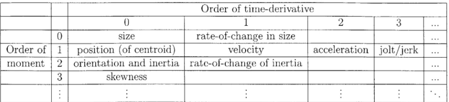
Order of time-derivative

0 1 2 3

0 size rate-of-change in size

Order of 1 position (of centroid) velocity acceleration jolt/jerk moment 2 orientation and inertia rate-of-change of inertia

3 skewness

Table 4.1: Exhaustive set of features for representing object silhouettes.

are the moments themselves. Moments of all orders, along with their time derivatives of all orders, contain complete information for characterising any tracking sequence. An illustration of this exhaustive set of features, as well as names for some of the commonly encountered members of this set, is given in Table 4.1.

It should be noted that since second and higher order moments have been nor-malised for scale-invariance (as discussed above), their time derivatives will also be normalised. Derivatives of silhouette size (the zeroth order moment) can also be normalised by dividing by the silhouette size.

So far we have ignored the information present in the object's appearance (i.e. pixel-values within the foreground region). We now add a few descriptors such as average foreground and background intensity and hue, and their time derivatives; the complete list is given in Table 4.2, where most of these features are shown to contribute little to the classification task.

In practice, it is not possible to accurately calculate very high order spatial mo-ments from image data. To approximate the contribution of high order momo-ments, we introduce an extra feature: percentage occupancy. This is defined as the percentage of pixels corresponding to the object silhouette within the smallest principal-axis-aligned bounding rectangle around the silhouette.