Cost Performance of Automobile Engine Plants

INTERNATIONAL MOTOR VEHICLE PROGRAM

FY

IMVP WORKING PAPERS

COST PERFORMANCE

OF AUTOMOBILE

ENGINE

PLANTS

Daniel Whitney Guillermo Peschard

and Denis Artzner

COST PERFORMANCE OF AUTOMOBILE ENGINE PLANTS

Daniel E Whitney Guillermo Peschard

Denis Artzner

Center for Technology, Policy, and Industrial Development Massachusetts Institute of Technology

Cambridge MA 02139 0 MIT 1997

Abstract

This paper analyzes the basic performance of 27 automobile engine lines operated by 18 companies on three continents, based on questionnaire data gathered in the Spring and Fall of 1995. Engine plants differ from assembly plants in being very capital-intensive. Thus a traditional “hours/engine” metric of performance is inappropriate. Here a composite cost comprising labor and amortization of capital, accounting for downtime, is used to compare plant performance. We find that performance varies widely, even for similar engines. Cost drivers comprise number of workers, capital

invested, and efficiency (fraction of scheduled time actually used for production). The drivers are in turn driven by external factors out of the plant’s control and internal factors that are under its control to some degree. We find that about half the variance in cost is due to the external factors, such as number of cylinders, utilization of scheduled time, and number of variants of engine made (the last loosely related to age of the engine family). Internal factors such as work in process inventory (strongly) and age of the workers (somewhat) drive cost. Downtime, the reverse of efficiency, is itself divided into scheduled and unscheduled downtime; the former is driven largely by number of variants while the latter is driven to some degree by the age of the family. The results of this study include a methodology to estimate the cost of variety. Statistical analyses are used to calculate the additional cost of

machining blocks ($4.92 more per block, $15 million extra investment, 9 additional workers and -4?40operating efficiency associated with one

additional square root of number of variants). This methodology can be extended to create a cost of variety for an entire engine.

This study was sponsored by the International Motor Vehicle Program. The authors gratefully acknowledge its support.

L Introduction

A. Background

The International Motor Vehicle Program’s (IMVP) current research efforts examine five broad areas in the industry: Product Development; Supplier Relations; Manufacturing, Organization and Human Resources; Distribution; and Environmental Issues. Within Manufacturing, the IMVP has studied the productivity of assembly plants for nearly a decade. In 1993 the program launched studies of two other important value-adding segments of automobile production: stamping plants [Roth] and engine plants. These new studies broaden the reach of the program by including capital-intensive operations that feed assembly plants and are sometimes directly integrated into them. This paper is the first to provide detailed information about engine plants. By contrast, data available in the public domain or from consultants cover fewer aspects of plant operations and performance or are not normalized with respect to standard operations or work content of the engine.

This study was conducted during the period June, 1994 to June 1997,1 and includes data from 27 engine families made in 18 plants on three continents, or about a quarter of all engine families world-wide. Ten companies took part in the study and contributed questions to the questionnaire.2 Details of the study’s methods and results may be found in [Peschard].

B. Methodology

The study was carried out using a mail questionnaire and follow-up visits or clarifications by fax. The questiomaire contained three parts:

1. Basic info-n about the Dkmt, its oDerating schedule , numb er of .

D1OV=SD(VfO~Ulg . .

standard aetm@es. and dadv schedule o. f work and break ~eriods. The

concept of “standard activities” was borrowed from the IMVP Assembly Plant Study. The purpose is to count the same activities in every plant, eliminating differences such as whether a plant makes its own cylinder heads (a standard activity), its own pistons (not a standard activity), and so on.

2. ~le . to an mdnndual e. . .

t~w’ An engine family is defined as all engines ha%g the s&ne a e fa.mflv m de at

1 The study’s phases were as follows: June, 1994- December, 1994 formulation of the

questionnaire in coninhtion with the partiapants; December, 94- December, 95: gathering and correcting data; March, 1995- June 1995: fixst phase of data analysis; June, 1995- June 19%: second phase of data analysis; June, 1996- June, 1997 third phase of data analysis

2The questionnaire is based on that of the IMVP Assembly Plant Study and borrows certain formats and questions from one developed by Opel Contributiona and advice from these sources are gratefully acknowledged.

3 These questions were answered individually for each engine family mad? at the plant.

number of cylinders and the same distance between cylinder centerlines. These questions include history of the family, descriptions of the family members currently being made, part count, complexity of operations, cost distributions among parts, labor, capital, and other costs, number of workers involved in standard activities, statistics about the shops (number of

machines, shop area, investment in equipment, distribution of operating and down time, and number of automated operations.

3. Questions on a varietv of toDics related to human resources, lofistics and mventories. maintenance ~roce dures. vrodu ction technolo~ies

(includirw how eau”~ment 1s obtained), aualitv, information svstems,

accountirw m actices . and recent immovement efforts. Of particular interest in this section are questions concerning length of supply lines, selective assembly, and patterns of involvement of plant personnel in plant design activities.

No attempt was made to define a “standard engine.” Instead, data were gathered and analyzed separately based on the number of cylinders (4, 5,6, or 8 in our sample). Regressions, discussed below, indicate that the number of cylinders explains a large part of the variation in manpower and cost per engine, confirming our decision to treat different cylinder numbers separately.

Responses to the questionnaire were analyzed directly in order to obtain a picture of typical plant operations. Regressions were then calculated on engine block machining in order to determine what correlations might be found. For this dataset, a composite cost was calculated, based on combining labor and equipment depreciation, scaled for scheduled utilization and

uptime! The costs and their correlates were divided into those directly under the control of the plant, such as age of the plant, work-in-progress inventory (lVIP), and age of the workers? and those determined elsewhere, such as factors inherent in the design of the engine, the number of variants in one family, and scheduled utilization.

Other analyses were conducted in order to determine root causes for certain performance results, such as downtime, and to see if certain

hypotheses (for example, does increasing variety in a plant increase the cost of making engines there) are true.

c

1. General Findings

QEngines are complex systems, typically containing 350 to 450 parts. Their cost to the assembly plants ranges from $600 to $2000. Most of the key parts are made by suppliers. Generally, engines are robust, and a properly

‘ Utilization and uptime are defined in Section IV.

5 C)f course, these factors are not altogether under the control of the plant, but they are local to the plant.

maintained plant with a well-trained and motivated workforce can make high quality engines regardless of many daily inconveniences and local problems.

. Engine plants are generally treated as captive suppliers. In most cases, plant managers and supervisors feel a lack of control over the factors that affect the plant the most: plant design, plant equipment choice, engine design, number of engine variants, and production schedules. W%en asked if they could calculate the cost of adding a variant, all said “No.”

● Engine plants differ greatly from assembly plants, having a lot of costly

capital equipment that is heavily stressed. Good cooperation and institutional learning by the workforce are important for keeping this equipment up and running and making good parts.

● Engines and engine plants last a long time. The average age of the

engine families in our sample is 12 years (std deviation 9 years). Many old plants operate well and make good engines. Many old engine designs are still being made and sold successfully.

c There is very wide variation in engine plant performance, whether measured according to total person-hours required to make an engine, amount of capital required to build one, amount of inventory, or percent uptime of equipment.

● Plant performance depends in complex ways on the engine’s design,

the age of the plant and of its workers, the design of the machines, and the number of different varieties of engine made. However, performance

variations between plants that make similar engines are larger than most of these individual effects can account for.

QEngine plants that manage - or are forced to manage - based on a single metric, such as hours per engine, may be forced to make ill-advised tradeoffs between labor and capital. For example, reducing labor available for

preventive maintenance will lower equipment availability, reducing overall effectiveness.

. Plant design and operating philosophies differ widely, with two identifiable camps distinguished by whether the plant’s owner directly controls a machinery vendor or not. Those that do (such as Toyota and Honda) generally have smaller, more manageable plants with fewer workers. There is some anecdotal evidence that they operate their plants according to principles and beliefs that are essentially unknown at other companies!

● The engine plant itself is responsible for only about 25°/0of the cost of

an engine. This amount is about equally split between labor costs, capital depreciation, and all miscellaneous costs (mainly consumables and scrap). The other 75% is purchased raw materials (2YXO)or finished parts and

6 These and other anecdotal issues are discussed ina separatepaper. .

subassemblies (50Yo). Therefore, to understand engine costs requires

broadening the unit of analysis beyond the plant to include engine design and the performance of suppliers, topics that are beyond the scope of this study.

c Suppliers not only provide half of the cost of an engine via value-adding finished parts and assemblies, but these parts embody most of the advanced technologies of engines (such as turbochargers, emission controls, fuel injectors, electronic timing, and fuel valving). In some cases the

suppliers control the technology through patents or know-how. One could say that the engine plants make mostly mature technology iterns and assemble the engine. The interface region between the new and mature tedmologies is the cylinder head, which may be said to be a battleground for control between the assemblers and the suppliers.’

. Put another way, engine plants make on the order of 5 to 7 of the 45o parts in a typical engine and devote half to three quarters of their capital and floor space to making them.

c Once we recognize the complexity of engines and the number of actors involved, we can predict the usefulness of studying other automotive

systems, such as chassis (not yet treated as a system by the industry), and trying to understand how control of them is likely to evolve and how their

control will influence future power flows between OEMS and suppliers.8 2. Detailed Findings from a Focused Analysis of Block Machining Lines The following findings apply to block machining lines and are supported by statistically significant correlations at the 0.05 level or bette~

. The type of engine (number of cylinders), the level of variety (measured as the square root of the number of variants) and the level of equipment utilization contribute to close to half of the variation in cost-perforrnance across plants.

. Work-in-Process (WIP) inventory appears to be a significant

determinant of performance and is closely associated with cost. Also, it is positively correlated with the number of workers and the amount of investment required. Moreover, the level of WIP inventory seems to be determined in part by the level of variety, which suggests that part of the influence of variety on performance takes its effect through a higher level of inventory.

. Of the equipment polities and characteristics tested, the age of the plant seems to be the most closely associated with performance: older plants are associated with lower efficiency and higher cost per block. The number of machines on the block line is an important determinant of the number of workers but does not have a visible effect on investment, efficiency, or cost.

7 See footnote 6. 8 See footnote 6.

Flowtime through 0.011 for the block

the shop is positively correlated with total downtime (p = line). However, contrary to expectations from several participants, cycle time of machines does not seem to affect either scheduled or unscheduled downtime. Other factors such as the use of Total Productive Maintenance programs and the level of cumulative production do not appear to have a significant effect on performance in our sample.

. Of the labor conditions we examined, absenteeism and the age of workers appear to be the significant variables. More absenteeism and higher age are associated with lower efficiency and higher cost per block. The

existence of incentive programs and number of hours of training per workers were also tested for an effect on performance but did not yield any statistically significant results.

. Finally, we examined the trade-offs between the factors that directly affect performance: the number of workers, investment and efficiency. We find that there are some visible trade-offs among the “resources” in our sample: workers can be replaced by investment, and workers can be added to the lines in order to improve efficiency.

3. Findings Determined from Data Applicable to Various Aspects of Plant Operation

Data were obtained on uptime of machining lines. Downtime was divided into scheduled (such as tool changes and fixture changes),

unscheduled (resulting from breakdowns), and employee break time. The following conclusions are supported at the 0.1 level or better:

. The number of unique engines in a family correlates positively with the age of the engine family (p = 0.11). This confirms statements made to us by many engine plant personnel, some of whom referred to “creeping

variety” as their main long term problem. Engine plants cost a lot and must be operated for many years in order to pay for themselves. The result is that engine families tend to last a long time, and many changes and additions are made over the years. This makes engine plants fundamentally different from assembly plants, which are rebuilt every 5 to 7 years, and stamping plants, which can accommodate new panel designs by using new relatively

inexpensive dies in the same relatively expensive presses.

. Scheduled downtime is positively correlated with the number of different varieties of iterns being made. For example, scheduled downtime on the block, head, and crank machining lines correlates positively with number of different kinds of blocks, heads, and cranks respectively. A

stronger correlation on the block line is obtained with the sum of the number of bores and strokes made (p = 0.007). A reasomble explanation is that

different varieties require different cutting tools and/or fixtures to be installed in the machines, req&ring them

Macintosh HIXMVP Save StuH3@ne Paper

. Unscheduled downtime correlates positively with total flowtime for heads and cranks through their respective machine shops. The sum of scheduled and unscheduled downtime correlates with flow time even better: for heads p = ().03, for cranks p = 0.06, and for blocks p = ().()11.@e ~os5ible explanation is that longer flowtirnes are associated with larger shops, for which it takes longer to transport people or equipment from place to place.

. Unscheduled downtime is also positively correlated with the age of the engine family (p = 0.08). Presumably this is due to the increased age of the machinery. Electrical failures occur more frequently early in a line’s life, and mechanical failures tend to dominate as a line ages.

. Unscheduled downtime in block (p = 0.07), crank (p = 0.09), and head (p = 0.05) machining also correlates positively with the fraction of workers in the respective shops that do non-production tasks. A possible explanation is that when a breakdown occurs in a shop with mostly production workers, it is they who either fix the breakdown or start repairs without delay. In either case, this saves time waiting for a non-production crew to arrive. A broader explanation is that one team is responsible for all the necessary tasks in a shop, learns them well, and takes total ownership of their shop.

● Reported hours/engine correlates positively with square meter area of

shops. One possible explanation is that larger shops require more people to cover them.

D. Organization of the Paper

Section II describes engines briefly, providing an overview of their parts and construction, basic engine cost distributions, and the costs and time required to design and build them. Section III briefly describes engine plants, listing the major departments, typical size of plant and workforce, and the time and cost required to design and build them. Section IV defines the plant performance metrics we derived from our data and analyzes them and their implications statistically. Section V concludes the paper.

IL Description Of Engines

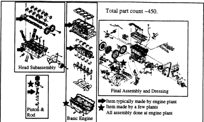
Engines are typically highly stressed, carefully designed products that must be carefully made. Figure 1 shows an engine and its main parts. The “basic engine” or “short block’ typically contains 250 to 300 parts, of which the engine plant usually makes the “5 C’s” comprising cylinder block, cylinder head, connecting rods, crank shaft, and cam shaft(s). Tolerances on these parts are tight, often a few microns, and continuous attention to dimensional quality is essential. Some plants make the pistons but none makes the piston rings, fasteners, seals, valves, springs, rocker arms, or other small or

specialized parts.

Figure 1. Main Parts of a Typical Four Cylinder Inline Engine

When the cylinder block is iron, it is the foundation for the entire engine, and almost all the other parts are attached to it with greater or lesser required precision. It therefore must be very carefully made. When the block is aluminum, the current trend, it is less stiff and unable to play the role of basic foundation by itself. The head, the crankcase, and the bolts that connect them comprise a structural unit whose design requires advanced engineefig and computerized methods. For aluminum engines, careful fabrication and assembly are both essential to obtain basic alignments and tolerances.

The moving parts of the engine (crank shaft, cam shaft(s), valves and valve linkages, and so on) move so fast that they must also be carefully designed, made and assembled in order to deliver low internal friction, vibration and noise, and wear. Cleanliness during fabrication and assembly are particularly important. Crankshafts are so hard to make that their scrap and rework rates are typically twice those for heads and blocks.

External to the basic engine are many parts involved in providing fuel, removing exhaust, providing electricity and controls, as well as sensors that monitor performance, plus auxiliary items like alternators, water and oil pumps, air conditioning compressors, and power steering units that take their power off the crank shaft via belts or gears. Almost without exception, these items are obtained from other companies or other divisions of the OEM and added to the engine in a phase called dressing. Since these items vary

tremendously across varieties of engines produced on any one line, the management of these parts’ inventories and the prevention of assembly errors comprise important activities of plant personnel.

Development of a new engine is a major investment requiring several years and upwards of $1 billion, including the cost of a new plant. Design focuses on improving performance and reducing weight. Weight reduction efforts show up in the shift from iron blocks and heads to aluminum, and the shift to advanced polymers in some lower temperature items such as intake manifolds. Thinner walls are also being designed into many castings,

requiring advanced methods of casting and machining. Some of these trends can be seen in lower amounts of material being machined off blocks and heads.

In Description Of Engine Plants

Most engine plants supply finished engines to a few vehicle assembly plants. A typical large engine plant employs a total of 300 to 1000 workers on one to three shifts, and makes from 200,000 to 700,000 engines per year. It consists of machining departments for the 5 C’s, a basic engine assembly department which adds the parts shown in the center of Figure 1, a cylinder head subassembly department, a final assembly and (not always separate) dressing department which adds the parts shown on the right in Figure 1, and a final test department. These departments vary in floor area, with some

plants being in total less than half the size of others with similar annual production capacity of similar engines.

Engine production is a significantly capital intensive activity. A typical engine plant requires from $300 to $800 million in capital investment in equipment and facilities. For this reason, it is a very long term asset with significant economies of scale.

The machining area of an engine plant is the more capital-intensive part it typically employs from one third to half of the labor in the plant (290 workers on average), and accounts for as much as 80°/0of the capital

investment. The machining shops can occupy from 50°10to 70% of a plant’s floor area. The assembly area employs the remaining one half to two-thirds of the labor and accounts for between 10% and 30°/0of total capital

investment.

The cylinder head subassembly consists of the cylinder head, the valve train, and the camshaft(s), and has (for an 14) roughly 170 parts. This

subassembly is usually built on a separate line. The piston/comecting rod subassembly has about 48 parts including the pistons, piston rings, connecting rods, and pin. It is usually assembled on a sub-line next to the basic assembly line.

The final assembly of the engine is typically the most manual activity in an engine plant. Roughly 150 to 250 parts are mounted on an engine in this part of the process which includes the following types of operations:

●install water and oil systems (pumps, seals, tubes, gages...) ●install manifolds (intake and exhaust)

●mount electronic system (alternator, distributor, spark plugs, harness, controller.

●assemble flywheel

●m(x,mt fuel injection system

Most plants conduct a hot test of their engines for 3 to 10 minutes after they are fully assembled. In general, more than 99°/0of the engines pass on the first run. Most plants hot test all their engines; however, a few plants only test 20% to 509f0of the engines, and some (not in our sample) do not hot test at all.

After find assembly and testing, finished engines are taken to the

shipping dock where they are packed and sent to the vehicle assembly plants. Only a few engine plants are located directly adjacent to assembly plants.

Iv. Plant Operating Data and Analyses

A. Definition Of Metrics

In order to properly measure the performance of an engine plant, it is necessary to appreciate the different pressures on its management and employees. They must balance the costs of labor and capital ~d must do so

under conditions in which many of the determining decisions have been made elsewhere by others. Figure 2 shows that only 25% of the cost of an engine is determined inside the engine plant itself. The design of the engine determines the difficulty of machining and assembling it, and the

performance of suppliers contributes greatly to cost and schedule

performance. To try to determine what is under the control of the plant and to see how different plants respond, we have defined four metrics of

performance.

Figure 2. Cost Distribution of a Typical Engine

1. Labor Productivity

Labor productivity is defined as the number of actual employee hours per year, including breaks and sick time, required to perform the following standard activities, per engine produced by the plant on average over a year: machining of the 5 C’s; accomplishing head subassembly and piston/

connecting rods subassembly; basic assembly of engine; final assembly and dressing; and hot test. From the questionnaire replies, we calculated the metric “hours per engine” and compared it with the plant’s own estimate of the same thing. In many questions, we distinguished between the number of workers assigned production tasks (production workers, PW) and the total number of workers (total workers, TW) assigned to a line.

2. Capital Productivity

Capital productivity is intended to measure the amount of capital that is invested in a plant or line per unit of capacity. This measure is expected to capture the differences between heavily automated plants that require a lot of investment, and more manual lines which may require less investment.

3. Eftlciency Of Plant Use

The efficiency of a line is meant to reflect the fraction of the parts that could theoretically be produced at full capacity compared to the number that are actually produced. For example, if the capacity of a line is 100 jobs per hour and on average 75 parts are produced per hour of operating time, then the efficiency of this line would be 75Y0. Thus, we calculated the efficiency of the lines as the ratio of the actual average production rate (jobs per hour) over the theoretical capacity of the line. We also defined “uptime” as another measure of the “effiaency” of the lines based on a different approach. Uptime is

defined as the time that is scheduled for production including overtime minus the time when the line is stopped for either scheduled or unscheduled downtime. The ratio of uptime over available time serves as a measure of the ability of a plant to keep the lines running when they are intended to be.

4. Cost Performance .

While single-factor productivity measures are useful to the extent that they permit simple comparisons across plants, they do not fully capture overall productivity. In order to obtain a measure that better captures overall productivity, it is necessary to use a measure that integrates all the relevant inputs (labor, capital, materials, energy. ..).

Based on the measure of total factor productivity (TFP) proposed by [Chew, Bresnahan, and Clark (1990)], we may construct a typical measure of the following form:

TFPi = [ (value ~ x sum (Cxi , X7) + (value ~x sum (CYj . Yij)] /[ (number of worker hours x wage + investment x cost of cap”tal + energy cost + materials cost];

where X and Y would be two main types of products,

valuex and ualuey would be monetary values assigned to product X and Y, and Cti would be a complexity factor assigned to each product subtype.

In our study, as in Chew et al, we only included labor and capital in our measure. Moreover, we have treated each plant as if it produced only one type, or family, of engines. Since the effect of product complexity is one of the issues that we are trying to examine, we have excluded the complexity factor from our measure and analyzed complexity separately using number of cylinders as a proxy.

The result is the following total factor cost formulation:

COSti= (~i X Wagei X Util.: + investi X capital_cost) / (CUplx ~ x Utill) (eq. 1)

where Costi is the calculated cost per unit at plant i;

~agei is the total cost to plant i for an average worker (based on local labor cost - wages and benefits - converted to US dollars); TWi is the total number of workers involved in standard activities;

utili is the utilization rate calculated as the share of total hours that are made available for production, where we considered that the total number of hours is 24 hours per day, 7 days a week.

inuestf is the total investment (in US dollars) in standard activities departments;

capita l_cos t is the cost of capital charged to the investment per

unit of time. In this case, the value used was capita l_cost = 10’% / year =0.00114% per hour, considering 24 hours per day, 365 days per year.

Capiis the capacity per unit of time, jobs per hour (JPH) in this case, calculated as the inverse of the theoretical cycle time. For example, if the plant’s theoretical cycle time is 30 seconds, then

capi = 30 seconds per unit x 3600s / hour = 120 units perhour;

e~~iis the efficiency of plant i, or the relevant line in plant i, measured as the fraction of capaaty that is achieved during the time available for production, thus,

ejf= actual production of good parts (]PH) / capacity (JPH)

B. Statistics On Manpower and Time Per Engine

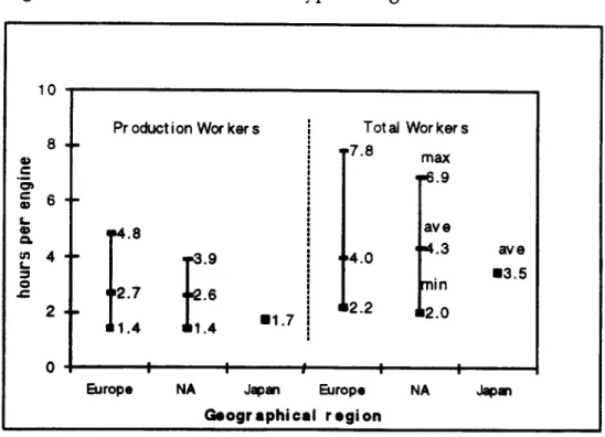
As documented in [Roos, et al], IMVI? researchers found during the late 1980’s that Japanese automotive companies’ vehicle assembly operations were significantly more productive than those of American and European firms. More recent studies of vehicle assembly plants, however, seem to point at a strong process of convergence. The best American and European plants seem to match the levels of labor productivity of the best Japanese pknts. Our results for labor productivity seem to confirm this: as shown in Figure 3, we have not found any significant regional differences, and the best plants in each region reach similar levels of productivity. In addition,

variation in labor productivity within regions seems to be far greater than that across regions. Note that among our sample of 27 families, six are made at “transplants” (plants whose owning company headquarters are in a

different country). The owning companies are in the US, Japan, and Europe. Anecdotal observation indicates that none of these owning companies has much difficulty imposing its operating philosophy on its distant plant.

Figure 3. Hours Per Engine for All Types, Separated by Geographic Region

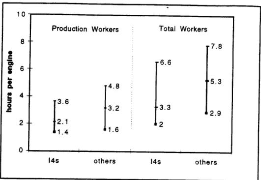
The number of cylinders is likely to affect the labor productivity of a plant: the more cylinders, the more operations that need to be performed and the more parts that need to be assembled and thus the more labor will be required. Our labor productivity data confirm this hypothesis to a certain extent. On average, as shown in Figure 4, engine plants producing 4 cylinder engines require 1/3 less labor per unit than plants producing larger engines. Significantly, there are plants that can produce large engines with far less labor than some plants can produce small engines.

Figure 4. Hours Per Engine for All Geographic Regions Based on Number of Cylinders

The most striking thing about Figures 3 and 4 is the wide range of labor productivity across plants in the same regions making engines of similar complexity.

c. Statistics On Required Investment

.

Total investment should include all investments in equipment and installation as well as upgrades to the line. However, since it requires accurate information on the amounts and times of investment, which are hard to obtain, we have relied on each plant’s estimate of the value of their line if they had to purchase it again. Gathering this information accurately and in a comparable way has been particularly complicated for a variety of reasons: plants seem to have used different methods for calculating the value of their investment, some plants refurbished old equipment from another plant making investment figures look very small, currency fluctuations and time value of money have been difficult to adjust because of a lack of information about amounts and dates of investments, etc. Figure 5 shows the results for capital investment per unit of capacity for the departments performing the standard activities.

Given the uncertainty in our data, we have watched the popular press for new engine plant announcements, which often state the planned capacity, investment, and employment. Such information is also subject to

uncertainty, of course. For six plants giving values for all three items, hours per engine ranged from 1.4 to 9.8 (average 5.04) and for 12 plants giving only investment and capacity, the investment per capacity per shift ranged from $180,000 to $825,000 (average $481,691), all similar to our results?

Figure 5. Investment Per Unit of Capacity for Individual Lines and Total. D. Statistics On Uptime And Its Implications

Companies were asked to report their uptime and downtime in three categories: employee break time during which the line was stopped,

unscheduled downtime (for tool breakage or machine repair), and scheduled downtime (tool change, fixture change, or scheduled maintenance). From these data, companies calculated and reported their net uptime. Since companies were also asked to report the number of cycles that resulted in good parts, we have a check on the uptime data. In general, the

correspondence is good, but the lack of really good correspondence is cause for concern. In some cases there were errors which we corrected. In other cases it emerged that plant personnel were not in the habit of calculating uptime, much less sorting downtime into scheduled and unscheduled. This apparent inattention to such presumably vital data indicates that plant persomel

either do not realize the comection between uptime and overall cost, or else management at headquarters do not realize it and therefore neither demand that such data be recorded nor set targets for uptime. When targets are set, they are in the vicinity of 80Y0.10

9 While we cannot identify individual plants, we can say that company and regional patterns in the popular press items are similar to those in our data.

10Eighty five percent net uptime is considered hard to beat in any industry, whether the line is manual or mechanized.

Figure 6 shows data for block machining lines, where we have made an effort to remove errors. The wide spread of net uptimes is significant. The fact that uptimes within the range are about equally likely indicates that there is no convergence among plants. This divergence is not explained by any of the following factors: number of cylinders, choice of machining cycle time, amount of employee training (hrs/ yr), years that total productive

maintenance (lTM) has been in effect (usually less than 3 years), or the degree to which capacity is being utilized. Even more striking is the fact that uptime in crank and head machining correlates excellently with uptime in block machining. (Figure 7)

A possible explanation for the similarity of uptimes in these shops is that all shops in a plant operate at the rate needed to make the parts required. Since each engine needs one block, one crank and (for I’s) one head, and since the plant presumably was built with balanced capacity in all machining lines, if a plant needs only 75% of the block line’s capacity, then it should need only 75% of the crank and head lines’ capacity. But we find statistically that there is no correlation between uptime and percent capacity utilization, indicating that plants with low uptime make up their production needs by operating for longer hours. This suggests in turn that the similarity of uptimes across lines in the same plant is the result of management’s efforts (when uptime is high) or management’s neglect (when uptime is low).

Figure 6. Distribution of Uptime and Downtime in Engine Block Machining lines.

Figure 7. Correlation between Uptimes in Block, Crank and Head Machining.

E. Statistics On Cost Performance

Cost performance was analyzed carefully for block machining lines after special efforts were made together with the plants to remove errors from this section of the dataset. The complete set of analyses maybe found in

[Peschard]. Some significant results are reported here.

Using equation (l), a cost to machine a block was calculated for each family. The results are shown in Figure 8. As can be seen, there is an enormous variation in terms of cost-performance. The ratio between the highest and lowest values is in the order of 6:1, with an average of $33.12 per unit and a standard deviation of $15 per unit. The line labeled “cost adjust all” is discussed in the next section.

Figure 8. Distribution of cost per unit calculated for block machining lines. The line labeled “cost adjust all” shows the cost after the differences in cost due to number of cylinders, utilization, and number of variants (i.e., the external factors) have been removed.

Macintoah HDiM’VP Save StufkEngine Paper

In tracing the sources of cost variation, we looked first at some of the factors which are not under the direct control of the planti the level of capacity utilization, the complexity of the engine, and the level of variety. First, we looked at how these external factors affected cost-performance, and then we analyzed these effects by analyzing the effect on the three main drivers of performance: workers, efficiency and capital.

Capacity utilization may affect cost-performance in two ways. First, the obvious effect, as capacity utilization increases, the capital cost of the engine plant can be distributed over a higher number of units. This effect is more significant the larger the share of capital cost in total cost. Second, utilization may have an effect on the efficiency of the lines. As people at one of the plants we visited suggested, running an engine plant on three shifts limits the time available for maintenance, which may lead to more frequent stops for machine failures and thus a lower efficiency. We calculated capacity

utilization as the percent of total time (24 hours a day, seven days a week) that is made available for production, including overtime.11

The complexity of the engine may affect the performance of the plant to the extent that a more complex engine requires more operations, more

machines, thus more people and investment. A more complex engine may also require more complex operations which may be slower and may have a higher probability of machine or tool failure. Elements which could

contribute to the complexity of the product in block machining may include the number of cylinders, the number of holes, the complexity of the

machining operations required, or the tolerances necessary.12 In this study, however, we have focused only on the number of cylinders in order to capture the effects of the most obvious indicator of complexity of the cylinder blocks.

Variety in the products has been pointed at as an important reason for differences in productivity by various participants in our study. The more variants, the more often a line will need to stop for tool and fixture changes and adjustments, and the more investment may be necessary to provide flexibility to handle different products. Different technology choices may respond differently to variety, but we expect in any case to see a visible cost disadvantage associated with increased variety.

11Onaverage, the level of utdization in our sample was 55~0, with a minimum of27’?/oand a

maximum of 85% ~ a point of comparison, a plant which operates 2 eight-hour shifts, 5 days a week would have a utilization level of 48°L.

‘2 At one of the plants, for example, we were told that one of the main reasons for having lower than averageproductivitywasthattlieenginewasdifficultto manufacture.Afterthe engine

had been introduced in that plant, the design of the engine was improved using the experiences of this plant and the redesigned engine was introduced at a different plant. The plant producing the re-designed engine requires many less operations and approximately half the amount of labor of the original plant.

Using ordinary-least-squares regression, we estimated the effect of these variables on the calculated cost per block.- The model that we used in the regression was as follows:

Model 1: cost = AO + A ~ utilization + A2 cylinders + A3 square root uariants

wherecost is the measure of cost-performanceconstructedfor blocks as definedin equation1;

utilization is the measureof capacityutilizationas used in equation 1 for the constructionof themeasureof cost-performance;

cylinders is the numberof cylinders,whichin thiscase we use as a proxy for productcomplexi~; and

square root vaniznts is the squareroot of the numberof variantsof cylinder

blocks whichis usedas a proxyfor productvariety.’s

A 1, A2, and A3 are the coefllcients for utilization,cylinders, and variants respectivelyestimatedby theregressionon cost.

We selected an almostlinearmodelin order to make the results more intuitive: what is the effect of each additionalcylinder, of more variants.For example, each additionalcylinderis associatedwithan increaseof A2 in cost.

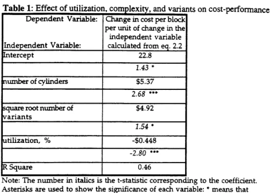
The results from the regression are shown in Table 1. The three variables show the expected signs. Utilization is negatively correlated to cost A one percentage point increase in the level of utilization is associated with a

reduction in cost per block of $0.448. This suggests that if one of the plants has below average utilization levels of, for example 35Y0, cost per block can be reduced by nearly $10 by raising utilization to the average of 55Y0. The

number of cylinders has a positive effect on cost, significant to a l% level. On average, each additional cylinder adds $5.37 to the cost of production of a block. Also, the number of variants shows a positive correlation with cost. Increasing the square root of number of variants by 1-- or increasing the number of variants from 1 to 4, or from 4 to 9 for example – is associated with an increase in cost of $4.92 per block.

The correlations with utilization rate and cylinders seems to be fairly strong, the probability of sign error is below lYo. The association with the number of variants is slightly weaker, but it is still significant the probability of sign error is 7’Yo.

u The square root form was used to allow for a diminishing effect of variants. After testing various functional forms of the number of variants, we found that the square root form had the best fit in most of our regressions, so we selected to use this form throughout tie study.

Table 1: Effect of utilization,complexity,andvariantson cost-perfo~mce DependentVariable: Changeincost per block

per unit of change in the independent variable Independent Variable: calculated from eq. 2.2

Intercept 22.8

2.43 *

number of cylinders $5.37

2.68 ***

square root number of $4.92

variants

1.54 *

utilization, YO -$0.448

.2.80 ***

R Square 0.46

Note: The number in italics is the t-statistic corresponding to the coeffiaent. Asterisks are used to show the significance of each variable: * means that the probability of sign error is between 5?!. and 10Yo,*’ between 1% and 5?4., and *** below lYo.

Another important result in this regression is the value of R2 of 0.46, which suggests that nearly half of the variance in cost can be attributed to these variables. (This fact is illustrated in Figure 8, where the cost per block has been adjusted to eliminate cost differences due to these three factors.) This would mean that half of the variation in cost-performance comes from factors which are not controlled by the plants: the level of utilization, the variety of products, and the level of complexity are generally determined by the demand that a company places on each plant, and by the design of the engine.

2. Effect of Internal Factors: Work in Process Inventory (lVIP)

Work-in-process inventory (wIF’) has been identified in recent years as one of the main elements of performance for a manufacturing facility. Part of the success of the “lean” production system has been attributed to the strict focus on reducing WTP to the lowest possible level.

WIP implies the existence of an unproductive capital investment. On average, the engine plants in our sample hold about $22 million in

inventory, $7 million of which consist of WIP. The distribution of total value of inventory is shown in Figure 9. Assuming a cost of capital of 15% per year and a production volume of 300,000 per year, $7 million in inventory would increase the cost of an engine by $3.50.

Figure 9. Distribution of Value of Inventory in Engine Plants

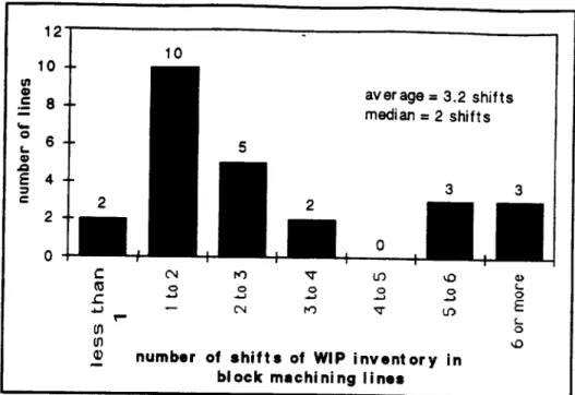
& shown in Figure 10, a typical block line carries two shifts of WTP inventory.

Figure 10. Level of WIP inventory on block machining In addition, WIP requires additional labor for handling

lines - histogram and aualitv control. The data from our sample seems to confirm these hypoti’eses:’ more WIP is significantly associated with more support workers and with more investment.

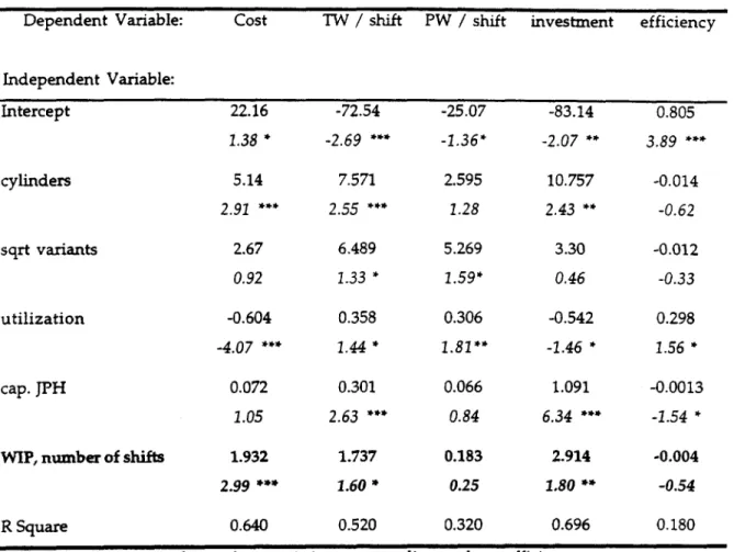
We used ordinary least squares regressions to analyze the effect of WIP on performance by including the number of shifts of WIP in the block machining lines into our regression model. As shown in Table 2, one additional shift worth of WIP inventory in the block machining line is

associated with 1.7 more total workers per shift. But WIP was not significantly associated with production workers, so we can presume that it is associated with 1.7 additional support workers, which may be in charge of the extra handling and control required. Also, one additional shift of WIP inventory is associated with an additional investment of $2.9 million, which may take the form of extra equipment necessary in order to deal with it.

As shown in Table 2, each additional shift of WW inventory on the block line is associated with a $1.93 higher cost per unit (significant beyond the 1% level). When compared to the results from Table 1, we can notice that when we include WIP in the model, the relevance of the number of variants decreases both in magnitude of the coefficient (from 4.92 to 2.67) and in significance (the t-statistic goes from 1.54 to 0.92). This may suggest that WIP is associated with more variety, which is investigated below. However, given that the R2 increases from 0.464 to 0.640 when WIP is included, we have concluded that the effect of WIP is not limited to the effect of variety: WIP significantly contributes to explaining the variation in cost-performance across plants.

In Table 2, we can also notice that WIP is not significantly associated with efficiency, which may suggest that two confronting effects balance each other. On one hand, more WIP may occur as a consequence of an unbalanced system with a lot of breakdowns in some part of the line, so WIP would tend to be associated with lower efficiency. On the other hand, WIP could be expected to be associated with higher efficiency since it may prevent certain disruptions of the entire line when one of the machines breaks down.

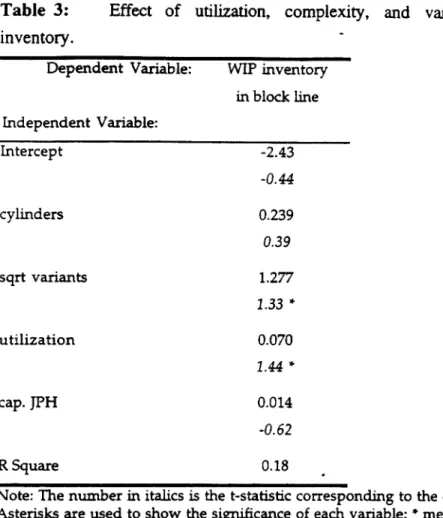
We then used ordinary least-squares regression to investigate the factors that may lead to high WIT. As shown in Table 3, the two factors that are most closely associated with WIP are utilization and variety. Each percentage point increase in the level of capacity utilization is associated with 0.07 shifts of additional WIP inventory. Also, increasing the square root of the number of variants by one unit (for example, going from 1 to 4 variants or from 4 to 9) is associated with adding 1.28 shifts of WIP inventory. Both coefficients are only slightly significant and have a probability of sign error close to 10’7o.The association of WIT and variety was predictable: more variety requires higher buffer levels to allow the same level of “coverage” to the flow on the line. The association of V/W and the level of utilization, on the other hand, is

-somewhat puzzling. Perhaps plants that -are under heavier demand pressure are running at higher level of utilization and allow themselves to hold larger buffers in order to keep production uninterrupted.

Table 2: Effect of WTPon performanceof block lines

DependentVariable: cost TW / Shift PW / shift investment efficiency

Independent Variable: Intercept 22.16 1,38 * -72.54 -2.69 *** -25.07 -1.36* -83.14 -2.07 ** 0.805 3.89 **” -0.014 -0.62 -0.012 -0.33 0.298 1.56 * -0.0013 -1.54 * -0.004 -0.54 0.180 cylinders 5.14 2.91 *** 7.571 2.55 “** 2.595 1.28 10.757 2.43 ** 2.67 0.92 6.489 1.33 * 5.269 1.59* 3.30 0.46 Sqrt variants utilization -0.604 -4.07 “*” 0.358 1.44 * 0.306 1.81** -0.542 -1.46 * cap. JPH 0.072 1.05 0.301 2.63 *** 0.066 0.84 1.091 6.34 ***

WIP,number of shifts 1.932 2.99 *** 1.737 1.60 * 0.183 0.25 2.914 1.80 ** 0.520 0.320 0.696 R Square

Note: The number in italics is the t-stadstic corresponding to the coeffiaent. Asterisks are used to show the significance of each variable: ●means that

the probability of sign error is between 5?’oand 10Yo,**between 1°70and 5Y0, and *** below IYo.

0.640

Table 3: Effect of utilization, complexity, and variants on Work-in-Process inventory.

Dependent Variabie: WIP inventory in block line Independent Variable: Intercept -2.43 -0.44 cylinders 0.239 0.39 sqrt variants 1.277 1.33 * utilization 0.070 1.44 * cap. JPH 0.014 -0.62 R Square 0.18 _.

Note: The number in italics is the t-statistic corresponding to the coeffiaent. Asterisks are used to show the significance of each variable: “ means that the probability of sign error is between 5% and 10Yo,‘“ between 1% and 5%, and **” below lYo.

F. Summary

External factors which can not be directly controlled by the plant (the number of cylinders, number of variants, level of utilization) are associated with almost half of the variation in cost-performance. The number of cylinders is associated with a higher cost per block, and it is correlated with more workers, more investment, and to a less certain extent to lower efficiency. An increase in the number of variants is also weakly associated with higher cost, more investment, and lower efficiency, and is significantly correlated to more workers. Finally, the level of utilization is associated with better performance: high utilization leads to lower cost since it is associated with better efficiency which outweighs the correlation of higher utilization with more investment and more workers.

Other factors which are under closer control by the plant also have an effect on cost performance. A higher level of WI? inventory on the block machining line was closely associated with a higher cost per unit, more workers (support workers), and more investment.

We also investigated various policies and characteristics relating to the equipment and facilities. The age of the plant appeared to have a negative effect on cost-performance. Other measures, such as cumulative production, the number of cutting machines, or the number of years of implementation of Total Productive Maintenance programs did not show a significant association with performance in our analysis.

Some labor policies and characteristics showed some associations with performance: older workers are associated with higher cost per block and lower efficiency. Similarly, higher absenteeism is correlated (weakly) with higher cost and to lower efficiency.

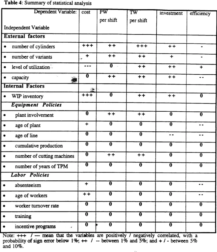
Table 4 summarizes the results of all our statistical analyses. Figure 11 graphically displays the most important pairwise and multiple regression relationships found in our study.

Table 4: Summaryof statisticalanalysis Depen&ntVariable: cost Pw

per shift per shift IndependentVariable External factors ● numberof cylinders +++ ++ +++ ++ . ● numberof variants _.=+ ++ ++ + . ● level of utilization- .-.

0-

++

++

+

o

++

++

++

-.

o

++

++

o

o

++

++

o

0

o

0

0

-.

0

0

.-

. .

o

0

0

0

0

o

++

++

o

0

o

0

0

0

0

o

0

0

. .

o

0

0

-.

o

0

0

0

0

training

o

0

0

0

0

0

t

o

0

0

0

Note: ~ / — mean that the variables are positively,/ negativelycorrelated with a probabilityofsign error below 1%, # I -- between 1% and 5%, and + 1- between5%

and 10%.

Figure 11. Graphical Summary of Factors Affecting Engine Plant Performance. (Based mainly on data for block machining lines)

G. Tradeoffs bong Drivers of Performance: Substitution of Resources

Given that our measure of cost-performance (equation 1) is actuauY constructed from efficiency, investment, and the number of workers, together with capaaty and utilization as well as local wages, it is logical that variation in cost can be explained by variation in these variables. However, it remains to be understood how each of these variables affects cost-performance. In order to quantify such effects, we used our cost function from equation 1 to calculate the change in cost per unit (called the marginal cost) that would arise from a unit change in each of our factors: workers, investment and efficiency.

The marginal cost per unit of a worker is a function of wage, as well as the level of capacity and efficiency. Based on eq(l), the marginal cost per unit of adding one worker is (partial derivative):

MCI unit

workm = wage / (capacity . eficiency) (eq. 2) Similarly, the marginal cost per unit of adding a million dollars of

investment, and of losing one percentage point in efficiency are: MC unit

= ($1 M . capital_c@) i (capacity . ejflciency . utilization ) irmedrncnt

(eq. 3) and

Mc ~:t ~=

- [(wage . # workers)/ (cap . ef 2,1- [( inv . capihzl_cost) / (cap .

util , eff2)] (eq. 4)

As shown in Table 5, each additional worker per shift adds on average $0.31 to the unit production cost of a cykder block (based on equations 2 to 4 and using the local labor cost corresponding to each plant converted to $US).

Table 5: Marginalcost of workers, effkiency and investment(based on equations2 to 4 usedon the datain our sanmle)

Marginal cost ok average lowest highest

Workers $0.31 $.03 $1.01

Efficiency $0.44 $0.15 $1.05

Investment $0.30 $0.17 $0.72

These results can also be read as:

If we could... while holding all eke the same we would save (on average)...

cut one worker per shift $0.31 per unit

improve eficiency by one percentage point $0.44 per unit

reduce investment required by $1 million $0.30 per unit

The question that immediately follows these results is how to reduce the work force, or improve efficiency, or reduce the investment. One possible path is to substitute resources for one another.

Substitution of resources - Tradeofis between workers, investment, efficiency

By substituting resources, we may for example be able to reduce the number of workers by adding investment in machinery. Or we may improve efficiency by adding workers to m+ sure the line stays up. Would these substitutions make sense? In order to resolve these questions through a benefit/cost analysis, we would need to know both the marginal costs of the “resources” (investment, workers, efficiency) and the rate at which we may be able to substitute a resource for another: the marginal rate of substitution.

Given the complexities of an engine plant, it is not possible to construct a measure of the marginal rate of substitution. On the factory floor, certain substitutions are possible, such as the choice whether to automate certain operations, or the decision of how many people to put in charge of operating and maintaining the machines. Moreover, most substitutions can not be multiplied or divided: being able to substitute an automatic station for one worker does not necessarily mean we can replace 10 stations with 10 workers, or half for half. Understanding these limita~ons

rate of substitution, we looked at our regression the tradeoffs among our resources.

1. Workers vs. investment

We had formulated the hypothesis that it is

of any estimate of a marginal results for some insight into

possible te a certain extent to substitute workers for investment, so we expected to see a negative

correlation between the number of workers and investment. This hypothesis was confirmed with the negative coefficient found for the investment in the regression for the number of workers [Peschard, Table 3.2, p 48]. One million dollars of additional investment is associated with between 0.16 and 0.24 less production workers (PW), and 0.13 less workers total (TW). The association with PW is also more significant than that with TW: the probabilities of sign error in the estimation of the coefficient are below 1°/0and above 10% for PW and TW respectively. This result makes sense to the extent that investment replaces operators (PW) so we can expect the relationship with PW to be more direct and thus yield more significant results.

Moreover, while additional investment in automation may reduce the need for operators, it may increase the need for indirect workers. In fact, automation such as robots for loading and unloading blocks into and out of the line, or to maintain buffer levels, which is the type of automation where substitutions may be possible in a block machining line, generally requires a lot of attention and maintenance, and thus more indirect workers. During various plant visits we were told stories of this type of automation being particularly unreliable, and at least in one case, the plant personnel simply

stopped using a robot to load blocks inte the line because they were not able to make it work appropriately. In sum, it seems understandable that investment is clearly associated with less operators while the association with total

workers is much less clear: does the reduced number of operators offset the increased number of indirect workers?

2. Efficiency vs. Workers and investment

We expected the number of workers to be positively correlated with efficiency, based on the hypothesis that if more people are available to work on the machines, the more likely they would be to keep the machines up and the less time it would take to fix machines or to change tools. The regression results in [Peschard, Table 3.3, p 50] seem to confirm this hypothesis. Both the number of production workers and total workers are positively correlated with efficiency One additional production worker (PW) is associated with an increase in efficiency of 0.5 percentage point while one additional total worker (TW) is associated with a 0.28 percentage point increase in efficiency. Even though regressions do not imply a causality link but a mere association, this association, significant beyond 5°/0(probability of sign error is less than 5% for the calculated coefficients) may serve to illustrate that reducing the number of workers may have a negative effect on efficiency.

Investment is also positively correlated to efficiency. An additional million dollars in investment is associated with an improvement in

efficiency of between 0.16 and 0.26 percentage points (significant at 5°/0level). This may suggest that incremental investments may help to improve

efficiency. Perhaps, efficiency can be increased by investing in more flexibility such as to reduce the time to change tools or to change variants, or in better controls to make it easier to monitor the machines and diagnose problems.

The relationships we have found can be summarized in Tables 6 and 7. Table 6. Summaryof SubstitutionEffects

A changeof... increasescostper andis associated (holdingall else the unitby.. with...

same)

+$1 MUSD $0.30 -0.14production -0.13 total +0.2percent

invesbnent workers(PW) workers(TW) points higher

efficiency

+1 Production worker $0.31 +0.5 percent points higher effiaency

+1 Total worker $0.31 +0.28 percent points higher efficiency

-1 percentage point $0.44 efficiency

Table 7. Summaryof DifferentialCost Impacts

A changeof... increasescost per and is associated (holding the

unit by.. with... other

characteristics the same)

+1 cylinder $5.37 +$14 million +9 workers -570 efficiency

investment

+1 Sqrt variants $4.92 +$15 million +9 workers -470 efficiency investment

-170 utilization $0.45 -0.4 workers -0.2’%0efficiency

v. Conclusions

A. There is a lot of variation in performance across plants.

The one feature that was shared by all measures of performance that we investigated was the existence of substantial variation from plant to plant. The ratio of highest to lowest cost-performance is 6 to 1, the ratio of highest to lowest hours per engine was approximately 3 to 1, and that of highest to lowest capital productivity was estimated in the order of 4 to 1.

B. Plants have remarkably little control over cost-performance.

Three quarters of the cost of an engine consists of purchased parts and components. These items are the responsibility of some centralized

department which negotiates with suppliers. Thus, the largest share of cost does not depend on the management of an engine plant. Other important factors, such as operating schedules and number of engine and part varieties, negatively impact performance and are not under the plant’s control.

C. Increased variety definitely increases cost

Statistically verifiable evidence suggests that increased variety increases costs in several ways: increasing scheduled downtime, increasing WIP, and increasing the number of workers needed.

C. Work-in-Process Inventory is a good indicator of performance

As in other studies, our statistical analysis attributed to WIP inventory a significant explanatory value. It is not clear which way the causal relationship goes: does good performance allow you to have low WiP, or is it low WIP that allows you to improve performance? As discussed above, it is probably a combination of both, and this association may suggest that plants that have focused more on lowering WIP have achieved better results.

Moreover, WIT inventory appeared to be a principal mechanism through which variety hurts performance: more variety is associated with more WIP, which in turn is correlated with poorer performance.

D. Labor policies and TPM

While we expected that certain policies such as Total Productive

Maintenance or Quality teams would have strong effects on performance of plants, our hypothesis was not supported by our data. However, it seems noticeable that all plants are adopting similar practices and policies with the same objectives: it seems that unlike the substantial difference in approaches between “mass” and “lean” production systems revealed in [Roos, et al], all plants in our sample on a first look seem to be following similar approaches.

E. Substitution of resources

Even in block machining shops, where transfer lines are used by most plants, certain substitutions among resources seem possible. Equipment could be utilized more effectively by investing in more flexible machines that may make changeovers quicker and reduce the labor required. Also, additional workers can be devoted to the maintenance of a line in order to reduce the downtime and thus increase efficiency.

Given that such substitutions are available, if plants are evaluated by some metric which focuses only on certain resources, they would have a somewhat metric-driven incentive to substitute certain resources for others, which may lead to a non-optimal results such as excess investment and lack of people. For this reason, single-factor measures may have adverse effects on a plant.

F. Cost of Variety

No one at any plant we visited could tell us the cost of adding a variant to the currently produced family of engines, leaving plant personnel unable to explain the impact to the rest of the company. In this paper, a statistical method was used to estimate cost of variety on block machining lines. T’he impact is substantial and verifiable statistically. This method could be extended to cover variety impacts elsewhere in the plant.

There is much more to be learned about engine plants, and engine plants can improve their operations. However, the opportunity to make major changes occurs only rarely. Too often, auto manufacturers do not take the time to consider their options carefully, but instead design their plants unsystematically and/or leave the responsibility for plant and line design to vendors. This and other topics are the subject of another paper.

VL References

[Chew, Bresnahan, and Clark (1990)] Chew, Bruce W., Timothy F. Bresnahan, and Kim B. Clark, 1990. “Measurement, Coordination, and

Learning in a Multiplant Network”, in Kaplan, Robert, 1990. Measures @

Mmzz@cturirzg Excellence, Harvard Business School Press, Boston, MA.

[Peschard] Peschard, Guillermo, “Manufacturing Performance: a Comparative Study of Engine Plant Productivity in the Automotive Industry: SM Thesis, Dept of Mech Eng, June 1996.

[Roth] Roth, Richard, Ongoing IMVP Study of Stamping Plants [Roos, et al] The Machine that Changed the World: the Stoy of Lean

Production, 1990, by James P. Womack, Daniel T. Jones, Daniel Roos, Rawson

Associates, New York, NY.

u

*A

d

Ohem ~ically madebyengineplant

Piston& * Itemmadebya fewplants

Rod Allassemblydoneatengineplant

Figure 1. Main Parts of a Typical Inline 4 Cylinder Engine (Courtesy Ford Motor Co.) Note how few of the parts are made at the engine plant.

Cost Distribution of s Typicsi Engine . 60% SOY. z g 30% 10Y. o“4. 1 55.0% madian (rein - max) 6.1% - 28.3Y+,8% - 7~)

Figure 2. Cost Distribution of a Typical Engine

Product ion Workers

: # 1 : ; !

‘[

I

.8

;:,

I

EuroFIo NA JSWI tirope NA JqMl

Geographical region

Figure 3. Hours Per Engine for All Types, Separated by Geographic Region

lo8 -: 5 : 6 -k 2 4--a 2 2-- 0--Production Workers ; 4.8 : 3.6 II 3.2 2.1 1.4 1.6 ‘ Total Workers

I

I

Figure 4. Hours Per Engine for All Geographic Regions Based on Number of Cylinders

Ax

Note: capacky per shift = 480 min x 60 “ $8i5

see/cycle time x 80% efficiency

I-1 l;j;;l;[;:;,::[; ;

( ‘

Figure 5. Investment Per Unit of Capacity for Individual Lines and Total.

1 2 3 4 6 6 7 8 14 1s 16 17 o 9 .

Figure 7. Correlation between Uptimes in Block, Crank and Head Machining.

---’”’”””~

g’

Figure 8. Distribution of cost per unit calculated for block machining line. The line labeled “cost adjust all” shows the cost after the differences in cost due to number of cylinders, utilization, and number of variants (i.e., the external factors) have been removed.

other tools,

consumables raw materials

finished engines 22?40 , purchased components 20% work in process 28’%

Average total inventory = $22 million

Figure 9. Distribution of Value of Inventory in Engine Plants

12] I 10 2 0 I 10 + average = 3.2 shifts median = 2 shifts 5 3 3 c m m v m-to” :

2

E

number of shifts of WIP inventory in block machining lines

Figure 10. Level of WIP inventory on block machining lines - histogram bxtema.1

factors

{

(+)

unscheciulee age of workers

Figure 11. Graphical Summary of Factors Affecting Engine Plant Performance. (Based mostly on data for block machining lines) Thicker arrows indicate stronger statistical significance.