Dispersion of mass and the complexity of geometric problems

(1)

Dispersion of Mass and the Complexity of

Geometric Problems

by

Luis Alexis Rademacher

Licenciado en Ciencias de la Ingenier´ıa

Universidad de Chile (2002) Ingeniero Civil Matem´atico Universidad de Chile (2002)

Submitted to the Department of Mathematics in partial fulfillment of the requirements for the degree of

Doctor of Philosophy at the

MASSACHUSETTS INSTITUTE OF TECHNOLOGY June 2007

c

The author hereby grants to MIT permission to reproduce and to distribute publicly paper and electronic copies of this thesis document in whole or in part in any

medium now known or hereafter created.

Author . . . . Department of Mathematics

May 1, 2007 Certified by . . . . Santosh S. Vempala Associate Professor of Applied Mathematics Thesis Supervisor Accepted by . . . .

Alar Toomre Chairman, Applied Mathematics Committee Accepted by . . . .

Pavel I. Etingof Chairman, Department Committee on Graduate Students

(2)

(3)

Dispersion of Mass and the Complexity of Geometric

Problems

by

Luis Alexis Rademacher

Submitted to the Department of Mathematics on May 1, 2007, in partial fulfillment of the

requirements for the degree of Doctor of Philosophy

Abstract

How much can randomness help computation? Motivated by this general question and by volume computation, one of the few instances where randomness provably helps, we analyze a notion of dispersion and connect it to asymptotic convex geometry. We obtain a nearly quadratic lower bound on the complexity of randomized volume algorithms for convex bodies in Rn_{(the current best algorithm has complexity roughly} n4_{, conjectured to be n}3_{). Our main tools, dispersion of random determinants and}

dispersion of the length of a random point from a convex body, are of independent interest and applicable more generally; in particular, the latter is closely related to the variance hypothesis from convex geometry. This geometric dispersion also leads to lower bounds for matrix problems and property testing.

We also consider the problem of computing the centroid of a convex body in Rn_.

We prove that if the body is a polytope given as an intersection of half-spaces, then computing the centroid exactly is #P -hard, even for order polytopes, a special case of 0–1 polytopes. We also prove that if the body is given by a membership oracle, then for any deterministic algorithm that makes a polynomial number of queries there exists a body satisfying a roundedness condition such that the output of the algorithm is outside a ball of radius σ/100 around the centroid, where σ2 _{is the}

minimum eigenvalue of the inertia matrix of the body.

Finally, we consider the problem of determining whether a given set S in Rn _is approximately convex, i.e., if there is a convex set K ⊆ Rn _{such that the volume}

of their symmetric difference is at most ² vol(S) for some given ². When the set is presented only by a membership oracle and a random oracle, we show that the problem can be solved with high probability using poly(n)(c/²)n _{oracle calls and}

computation time. We complement this result with an exponential lower bound for the natural algorithm that tests convexity along “random” lines. We conjecture that a simple 2-dimensional version of this algorithm has polynomial complexity.

Thesis Supervisor: Santosh S. Vempala

(4)

(5)

Acknowledgments

I would like to thank those that made this work possible.

To Santosh Vempala, my advisor, as this work is the result of our collaboration. To Madhu Sudan and Peter Shor, for being part of my thesis committee. To the Department of Mathematics and CSAIL at MIT and their members, for providing an environment that strongly stimulates research.

To my friends Amit Deshpande and Roberto Rondanelli, for interesting discussions around this work.

(6)

(7)

List of Figures

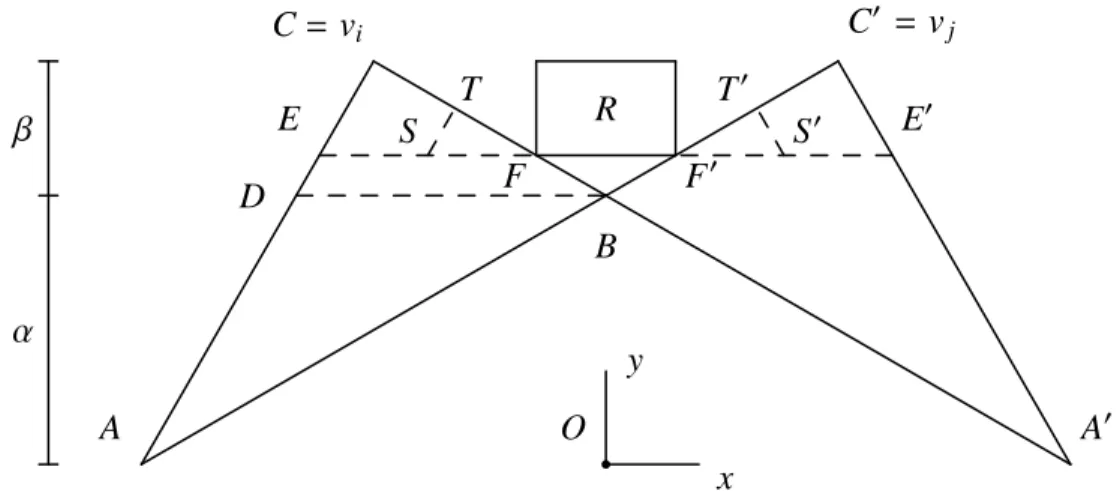
4-1 The 2-D argument. . . 46 6-1 Projection of the peaks (i, j) of the cross-polytope with peaks onto vi,

(10)

(11)

Notation

This is a list of symbols used frequently with their descriptions and, in parentheses, the numbers of the pages in which they are introduced.

Ri ith row (15)

R−i all rows but ith (15)

ˆ

R normalized rows (15) conv convex hull (15) vol volume (15)

D, D0 _{distributions (17)} Q membership oracle (16)

Q0 _{modified oracle (17)}

disp_µ(p) dispersion of a distribution µ (30)

K convex bodies and ∅ (60)

(12)

(13)

Introduction

Among the most intriguing questions raised by complexity theory is the following: how much can the use of randomness affect the computational complexity of algorith-mic problems? At the present time, there are many problems for which randomized algorithms are simpler or faster than known deterministic algorithms but only a few known instances where randomness provably helps. As we will see, one of these known instances is the geometric problem of computing the volume of a convex body in Rn

given by a membership oracle. One of the results of this work is another example where randomness provably helps: the problem of computing the centroid of a convex body.

The best known algorithm for approximating the volume of a convex body in Rn

has query complexity O(n4_{) [29]. The second and main contribution of this work is}

a lower bound of Ω(n2_{/ log n) for the complexity of approximating the volume. This}

lower bound actually holds for parallelotopes of the form {x : kAxk∞ ≤ 1}, for an n × n matrix A. As the volume of such a parallelotope is proportional to 1/|det A|,

what we actually give is a lower bound for the problem of approximating |det A| when

A is accessed through an oracle that given q ∈ Rn _{decides whether kAqk}

∞ ≤ 1. We

also give similar lower bounds for the problem of approximating the product of the lengths of the rows of A, and approximating the length of a vector.

To prove this lower bounds we introduce a measure of dispersion of a distribu-tion that models the probability of failure of an algorithm against a distribudistribu-tion on inputs. The computational lower bounds are then a consequence of two dispersion lower bounds that we prove: dispersion of the determinant of certain distributions on matrices, and dispersion of the length of a random vector from a polytope. This last results has interesting connections with an important open problem in asymptotic convex geometry, the variance hypothesis.

Finally, we study the problem of testing whether a set given by a membership oracle and a random oracle is approximately convex. We give an exponential time algorithm and we prove that a very natural algorithm that checks the convexity of the input set along random lines has exponential complexity.

The thesis is organized as follows:

Chapter 2 introduces some notation and basic results that will be used in the rest of this work.

Chapter 3 gives known deterministic lower bounds for the complexity of the vol-ume and gives our deterministic lower bounds for the complexity of the centroid.

(14)

properties of it and then proceeds to prove our two main dispersion results: dispersion of the length of a random vector from a polytope and dispersion of the determinant of a random matrix.

Chapter 5 uses the dispersion of the determinant to prove our lower bound for the complexity of approximating the volume.

Chapter 6 uses the dispersion of a random vector from a polytope to prove our other two randomized lower bounds, for the length of a vector and the product of the rows of a matrix.

(15)

Chapter 1 Preliminaries

1.1 Notation and definitions

Let S ⊆ Rn_{. If S is measurable, vol(S) denotes the volume of S. The convex hull of} S is denoted conv(S).

Let x · y = Pn_i=1xiyi, the usual inner product in Rn.

A parallelotope is any set that results from an affine transformation of a hypercube. Generally we will consider parallelotopes of the form {x ∈ Rn _{: kAxk}

∞ ≤ 1} specified

by an n × n matrix A. N(0, 1) denotes the standard normal distribution, with mean 0 and variance 1.

The n-dimensional ball of radius 1 centered at the origin is denoted Bn. We define πV(u) to be the projection of a vector u to a subspace V . Given a matrix R, let Ri

denote the i’th row of R, and let ˆR be the matrix having the rows of R normalized

to be unit vectors. Let ˜Ri be the projection of Ri to the subspace orthogonal to R1, . . . , Ri−1. For any row Ri of matrix R, let R−i denote (the span of) all rows

except Ri. So πR⊥

−i(Ri) is the projection of Ri orthogonal to the subspace spanned

by all the other rows of R.

1.2 Yao’s lemma

We will need the following version of Yao’s lemma. Informally, the probability of failure of a randomized algorithm ν on the worst input is at least the probability of failure of the best deterministic algorithm against some distribution µ.

Lemma 1.1. Let µ be a probability measure on a set I (a “distribution on inputs”)

and let ν be a probability measure on a set of deterministic algorithms A (a “random-ized algorithm”). Then

inf

a∈APr(alg. a fails on measure µ) ≤ sup_i∈I Pr(randomized alg. ν fails on input i).

(16)

Let I be a set (a subset of the inputs of a computational problem, for example the set of all well-rounded convex bodies in Rn _{for some n). Let O be another set (the}

set of possible outputs of a computational problem, for example, real numbers that are an approximation to the volume of a convex body). Let A be a set of functions from I to O (these functions represent deterministic algorithms that take elements in

I as inputs and have outputs in O). Let C : I × A → R (for a ∈ A and i ∈ I, C(i, a)

is a measure of the badness of the algorithm a on input i, such as the indicator of a giving a wrong answer on i).

Lemma 1.2. Let µ and ν be probability measures over I and A, respectively. Let

C : I × A → R be integrable with respect to µ × ν. Then

inf

a∈AEµ(i)C(i, a) ≤ sup_i∈I Eν(a)C(i, a)

Proof. By means of Fubini’s theorem and the integrability assumption we have

Eν(a)Eµ(i)C(i, a) = Eµ(i)Eν(a)C(i, a).

Also

Eν(a)Eµ(i)C(i, a) ≥ inf

a∈AEµ(i)C(i, a)

and

Eµ(i)Eν(a)C(i, a) ≤ sup

i∈I Eν(a)C(i, a).

Proof (of Lemma 1.1). Let C : I × A → R, where for i ∈ I, a ∈ A we have C(i, a) =

(

1 if a fails on i 0 otherwise.

Then the consequence of Lemma 1.2 for this C is precisely what we want to prove.

1.3 The query model and decision trees

We will denote by Q our standard query model: A membership oracle for a set

K ∈ Rn _{takes any q ∈ R}n _{and outputs YES if q ∈ K and NO otherwise. When K is}

a parallelotope of the form {x ∈ Rn _{: kAxk}

∞ ≤ 1} specified by an n × n matrix A,

the oracle outputs YES if kAqk∞≤ 1 and NO otherwise.

It is useful to view the computation of a deterministic algorithm with an oracle as a decision tree representing the sequence of queries: the nodes (except the leaves) represent queries, the root is the first query made by the algorithm and there is one query subtree per answer. The leaves do not represent queries but instead the answers to the last query along every path. Any leaf l has a set Pl of inputs that are

consistent with the corresponding path of queries and answers on the tree. Thus the set of inputs is partitioned by the leaves.

(17)

To prove our main lower bounds for the complexity of approximating the volume of parallelotopes, it will be convenient to consider a modified query model Q0 _that

can output more information: Given q ∈ Rn_{, the modified oracle outputs YES as}

before if kAqk∞ ≤ 1; otherwise it outputs a pair (i, s) where i is the “least index

among violated constraints”, i = min{j : |Ajq| > 1}, and s ∈ {−1, 1} is the “side”, s = sign(Aiq). An answer from Q0 gives at least as much information as the respective

answer from Q, and this implies that a lower bound for algorithms with access to Q0

is also a lower bound for algorithms with access to Q. The following definition and lemma explain the advantage of Q0 _{over Q.}

Definition 1.3. Let M be a set of n × n matrices. We say that M is a product set along rows if there exist sets Mi ⊆ Rn, 1 ≤ i ≤ n,

M = {M : ∀1 ≤ i ≤ n, Mi ∈ Mi}.

Lemma 1.4. If the set of inputs is a product set along rows, then the leaves of a

decision tree in the modified query model Q0 _{induce a partition of the input set where} each part is itself a product set along rows.

Proof. We start with M, a product set along rows with components Mi. Let us

observe how this set is partitioned as we go down a decision tree. A YES answer imposes two additional constraints of the form −1 ≤ q · x ≤ 1 on every set Mi. For

a NO answer with response (i, s), we get two constraints for all Mj, 1 ≤ j < i, one

constraint for the i’th set and no new constraints for the remaining sets. Given this information, a particular setting of any row (or subset of rows) gives no additional information about the other rows. Thus, the set of possible matrices at each child of the current query is a product set along rows. The lemma follows by applying this argument recursively.

1.4 Distributions and concentration properties

We use two distributions on n × n matrices called D and D0 _{for our randomized lower}

bounds. A random matrix from D is obtained by selecting each row independently and uniformly from the ball of radius √n. A random matrix from D0 _{is obtained}

by selecting each entry of the matrix independently and uniformly from the interval [−1, 1]. In the analysis, we will also encounter random matrices where each entry is selected independently from N(0, 1). We use the following properties.

Lemma 1.5. Let σ be the minimum singular value of an n × n matrix G with

inde-pendent entries from N(0, 1). For any t > 0,

Pr¡σ√n ≤ t¢ ≤ t.

Proof. To bound σ, we will consider the formula for the density of λ = σ2 _{given in}

[14]: f (λ) = n 2n−1/2 Γ(n) Γ(n/2)λ −1/2_e−λn/2_U µ n − 1 2 , − 1 2, λ 2 ¶

(18)

where U is the Tricomi function, which satisfies for all λ ≥ 0: • U(n−1 2 , −12, 0) = Γ(3/2)/Γ((n + 2)/2), • U(n−1 2 , − 1 2, λ) ≥ 0 • d dλU(n−12 , −12, λ) ≤ 0

We will now prove that for any n the density function of t = √nλ is at most 1. To

see this, the density of t is given by

g(t) = f µ t2 n ¶ 2t n = 2f (λ) r λ n = √ n 2n−3/2 Γ(n) Γ(n/2)e −λn/2_U µ n − 1 2 , − 1 2, λ 2 ¶ . Now, d dtg(t) = √ n 2n−3/2 Γ(n) Γ(n/2)× × · −n 2e −λn/2_U µ n − 1 2 , − 1 2, λ 2 ¶ + e−λn/2 d dλU µ n − 1 2 , − 1 2, λ 2 ¶¸ 2t n ≤ 0.

Thus, the maximum of g is at t = 0, and

g(0) = √ n 2n−3/2 Γ(n) Γ(n/2) Γ(3/2) Γ(n+2 2 ) ≤ 1. It follows that Pr(σ√n ≤ α) ≤ α.

Lemma 1.6. Let X be a random n-dimensional vector with independent entries from

N(0, 1). Then for ² > 0

Pr¡kXk2 ≥ (1 + ²)n¢ ≤¡(1 + ²)e−²¢n/2 and for ² ∈ (0, 1)

Pr¡kXk2 ≤ (1 − ²)n¢≤¡(1 − ²)e²¢n/2_.

For a proof, see [37, Lemma 1.3].

Lemma 1.7. Let X be a uniform random vector in the n-dimensional ball of radius

r. Let Y be an independent random n-dimensional unit vector. Then,

E(kXk2) = nr2

n + 2 and E

¡

(X · Y )2¢ ₌ r2

n + 2. Proof. For the first part, we have

E(kXk2) = R_r 0 tn+1dt R_r 0 tn−1dt = nr 2 n + 2.

(19)

For the second part, because of the independence and the symmetry we can assume that Y is any fixed vector, say (1, 0, . . . , 0). Then E¡(X · Y )2¢_{= E(X}2

1). But E(X2 1) = E(X22) = · · · = 1 n n X i=1 E(X2 i) = E(kXk2) n = r2 n + 2.

Lemma 1.8. There exists a constant c > 0 such that if P ⊆ Rn _{compact and X is a} random point in P then

E(kXk2) ≥ c(vol P )2/n_n

Proof. For a given value of vol P , the value E(kXk2) is minimized when P is a ball centered at the origin. It is known that the volume of the ball of radius r is at least

cn/2_rn_/nn/2 _{for some c > 0. This implies that, for a given value of vol P , the radius r}

of the ball of that volume satisfies

cn/2_rn

nn/2 ≥ vol P. (1.1)

On the other hand, Lemma 1.7 claims that for Y a random point in the ball of radius

r, we have

E(kY k2) = nr

2

n + 2. (1.2)

Combining (1.1), (1.2) and the minimality of the ball, we get Ã

c E(kXk2)(n + 2)

n2

!_n/2

≥ vol P

and this implies the desired inequality.

We conclude this section with two elementary properties of variance. Lemma 1.9. Let X, Y be independent real-valued random variables. Then

var(XY ) (E(XY ))2 = µ 1 + var X (E X)2 ¶ µ 1 + var Y (E Y )2 ¶ − 1 ≥ var X (E X)2 + var Y (E Y )2.

Lemma 1.10. For real-valued random variables X, Y , var X = EY var(X / Y ) +

(20)

(21)

Chapter 2 Deterministic lower bounds

2.1 Volume

About the possibility of exact computation of the volume, there are at least two negative answers. The first is that it is know to be #P -hard when the polytope is given as a list of vertices or as an intersection of halfspaces [11]. Secondly, one can construct a polytope given by rational inequalities having rational volume a/b such that writing b needs a number of bits that is exponential in the bit-length of the input [23].

About the possibility of a deterministic approximation algorithm with a member-ship oracle, the answer is also negative. The complexity of an algorithm is measured by the number of such queries. The work of Elekes [15] and Bárány and Füredi [4] showed that any deterministic polynomial-time algorithm cannot estimate the volume to within an exponential (in n) factor. We quote their theorem below.

Theorem 2.1 ([4]). For every deterministic algorithm that uses at most na member-ship queries and given a convex body K with Bn ⊆ K ⊆ nBn outputs two numbers A, B such that A ≤ vol(K) ≤ B, there exists a body K0 _{for which the ratio B/A is at}

least µ

cn a log n

¶_n

where c is an absolute constant.

We will see in Chapter 4 that there are randomized algorithms that approximate the volume in polynomial time, which shows that randomization provably helps in this problem.

2.2 Centroid

Given a convex body in Rn_{, the centroid is a basic property that one may want to}

compute. It is a natural way of representing or summarizing the set with just a single point. There are also diverse algorithms that use centroid computation as a subroutine (for an example, see [5], convex optimization). The following non-trivial

(22)

property illustrates the power of the centroid: Any hyperplane through the centroid of a convex body cuts it into two parts such that each has a volume that is at least a 1/e fraction of the volume of the body.

There are no known efficient deterministic algorithms for computing the centroid of a convex body exactly. We will see that this is natural by proving the following result:

Theorem 2.2. It is #P -hard to compute the centroid of an polytope given as an

intersection of halfspaces, even if the polytope is an order polytope.

(Order polytopes are defined in Subsection 2.2.1)

By centroid computation being #P -hard we mean here that for any problem in #P , there is a polynomial time Turing machine with an oracle for centroids of order polytopes that solves that problem.

On the other hand, there are efficient randomized algorithms for approximating the centroid of a convex body given by a membership oracle (See [5]. Essentially, take the average of O(n) random points in the body. Efficient sampling from a convex body is achieved by a random walk, as explained in [28]). We will see that no deterministic algorithm can match this, by proving the following:

Theorem 2.3. There is no polynomial time deterministic algorithm that when given

access to a membership oracle of a convex body K such that

1

17n2Bn ⊆ K ⊆ 2nBn

outputs a point at distance σ/100 of the centroid, where σ2 _{is the minimum eigenvalue}

of the inertia matrix of K.

(The inertia matrix of a convex body is defined in Subsection 2.2.1)

That the centroid is hard to compute is in some sense folklore, but we are not aware of any rigorous analysis of its hardness. The hardness is mentioned in [5] and [20] without proof, for example.

2.2.1 Preliminaries

Let K ⊆ Rn _{be a compact set with nonempty interior. Let X be a random point in} K. The centroid of K is the point c = E(X). The inertia matrix of K is the n by n

matrix E¡(X − c)(X − c)T¢_.

For K ⊆ Rn _{bounded and a a unit vector, let w}

a(K), the width of K along a, be

defined as:

wa(K) = sup

x∈Ka · x − infx∈Ka · x.

By canonical directions in Rn _{we mean the set of vectors that form the columns}

of the n by n identity matrix.

For a, b, c ∈ R, a, b > 0 and c ≥ 1 we say that a is within a factor of c of b iff 1

(23)

For a partial order ≺ of [n] = {1, . . . , n}, the order polytope associated to it is

P (≺) = {x ∈ [0, 1]n _{: x}

i ≤ xj whenever i ≺ j}.

In [9], it is proved that computing the volume of order polytopes (given the partial order or, equivalently, the facets of the polytope) is #P -hard. We will use this result to prove Theorem 2.2.

We will also need the following result for isotropic convex bodies, which is in a sense folklore (A convex body K ⊆ Rn _{is in isotropic position iff for random X ∈ K}

we have E(X) = 0 and E(XXT_{) = I). A proof can be found in [21].}

Theorem 2.4. Let K ⊆ Rn _{be a convex body in isotropic position. Then}

r n + 2 n Bn⊆ K ⊆ p n(n + 2)Bn.

2.2.2 Proofs

The idea of both proofs is to reduce volume computation to centroid computation, given that it is know in several senses that volume computation is hard.

A basic step in the proofs is the following key idea: if a convex body is cut into two pieces, then one can know the ratio between the volumes of the pieces if one knows the centroids of the pieces and of the convex body. Namely, if the body has centroid c and the pieces have centroids c−, c+, then the volumes of the pieces are in

proportion kc − c−k/kc − c+k.

It is known that the volume of a polytope given as an intersection of halfspaces can have a bit-length that is exponential in the length of the input [23]. It is not hard to see that the centroid of a polytope given in that form may also need exponential space. Thus, to achieve a polynomial time reduction from volume to centroid, we need to consider a family of polytopes such that all the centroids that appear in the reduction have a length that is polynomial in the length of the input. To this end we consider the fact that it is #P -hard to compute the volume of order polytopes. Lemma 2.5. Let P be an order polytope. Then the centroid of P and the volume of

P have a bit-length that is polynomial in the bit-length of P .

Proof. Call “total order polytope” an order polytope corresponding to a total order.

Such a polytope is actually a simplex with 0–1 vertices, its volume is 1/n! and its centroid has polynomial bit-length. The set of total order polytopes forms a partition of [0, 1]n _{into n! parts, and any order polytope is a disjoint union of at most n! total}

order polytopes. The lemma follows.

Proof (of Theorem 2.2). Let P ⊆ [0, 1]n _{be an order polytope, given as a set of}

half-spaces of the form Hk = {x : xik ≤ xjk}, k = 1, . . . , K. Suppose that we have

access to an oracle that can compute the centroid of an order polytope. Then we can compute vol P in the following way: Consider the sequence of bodies that starts with [0, 1]n_{, and then adds one constraint at a time until we reach P . That is, P}

(24)

Pk = Pk−1∩ Hk. In order to use the key idea, for every k, let Qk = Pk−1\ Pk, compute

the centroid ck of Pk and the centroid dk of Qk. We have Pk−1 = Pk] Qk and

vol Qk vol Pk = kck−1− dkk kck−1− ckk. Thus, vol Pk−1 vol Pk = kck−1− dkk kck−1− ckk + 1. This implies, multiplying over all k,

vol P = K Y k=1 µ kck−1− dkk kck−1− ckk + 1 ¶₋₁ .

The reduction costs 2K centroid oracle calls. Even though some expressions involve norms, all the intermediate quantities are rational (as the volumes of order polytopes are rational). Moreover, the bit-length of the intermediate quantities is polynomial in n (Lemma 2.5).

Proof (of Theorem 2.3). Suppose for a contradiction that there exists an algorithm

that finds a point at distance Cσ of the centroid. Then the following algorithm would approximate the volume in a way that contradicts Theorem 2.1, for a value of C to be determined. Theorem 2.1 is actually proved for a family of convex bodies restricted in the following way: We can assume that the body contains the axis-aligned cross-polytope of diameter 2n and is contained in the axis-aligned hypercube of side 2n. Let P be a convex body satisfying that constraint, given as a membership oracle. Algorithm

1. Let M = 1, i = 0, P0 = P .

2. For every canonical direction a: (a) While wa(P ) ≥ 1:

i. i ← i + 1.

ii. Compute an approximate centroid ci−1 of Pi−1. Let H be the

hyper-plane through c orthogonal to a.

iii. Let Pi be (as an oracle) the intersection of Pi−1 and the halfspace

determined by H containing the origin (if H contains the origin, pick any halfspace).

iv. Let Qi be (as an oracle) Pi−1\ Pi.

v. Compute an approximate centroid di of Qi.

vi. M ← Mkci−1−cik

kdi−cik

(25)

To see that the algorithm terminates, we will show that the “while” loop ends after

O(n log n) iterations. Assuming that C ≤ 1/2, at every iteration wa(Pi) decreases at

most by a factor of 1/(4n) (Lemma 2.9). Thus, Pialways contains a hypercube of side

1/(4n), and vol Pi ≥ 1/(4n)n. Initially, vol P0 ≤ (2n)n, and every iteration multiplies

the volume by a factor of at most 1 −1

e+ C (Lemma 2.8). Thus, the algorithm runs

for at most 2n log(n√8) log ³ 1 −1 e+ C ´₋₁ iterations.

We will now argue that for all the centroids that the algorithm computes, it knows a ball contained in the corresponding body. Let σ2

i be the minimum eigenvalue of

the inertia matrix of Pi. Initially, the algorithm knows that P0 contains a ball of

radius √n around the origin. Also, Theorem 2.4 implies that for every i, Pi contains

a ball of radius σi

p

(n + 2)/n around the centroid. Because Pi contains a hypercube

of side 1/(4n), Theorem 2.4 also implies that σi ≥ 1/(8n

p

n(n + 2)). Thus, after we

compute ci, the algorithm knows that Pi contains a ball of radius

Ãr n + 2 n − C ! σi ≥ Ãr n + 2 n − C ! 1 8npn(n + 2) ≥ 1 − C 8n2

around ci, and this implies that the algorithm knows that Pi+1, Qi+1 contain balls of

radius (1 − C)/(16n2_{) around known points.}

At step 3, Pi contains the origin and has width at most 1 along all canonical

directions. This implies that it is completely contained in the input body, as the input body contains the cross-polytope of diameter 2n. Thus, the volume of Pi is

easy to compute because it is a hypercube that we know explicitly at this point, the intersection of all the halfspaces chosen by the algorithm.

At every cut, kci−1− cik is within a constant factor of the true value, as the

following argument shows: Let δ2

i be the minimum eigenvalue of the inertia matrix

of Qi. Let ¯ci, ¯di be the centroids of Pi, Qi, respectively. We have that kci− ¯cik ≤ Cσi ≤ Cσi−1 and kdi− ¯dik ≤ Cδi ≤ Cσi−1. That is,

k¯ci−1− ¯cik − 2Cσi−1 ≤ kci−1− cik ≤ k¯ci−1− ¯cik + 2Cσi−1

and we also have that the true distance satisfies k¯ci−1− ¯cik ≥ σi−1/2 (Lemma 2.6).

Thus, the estimate satisfies:

(1 − 4C)k¯ci−1− ¯cik ≤ kci−1− cik ≤ (1 + 4C)k¯ci−1− ¯cik.

A similar argument shows:

(26)

Thus, M, as an estimate of V / vol P , is within a factor of µ 1 + 4C 1 − 4C ¶ 2n log(n√8) log(1− 1_{e +C)}−1

of the true value, and so is the estimate of the volume, V /M, with respect to vol P . The choice of C = 1/100 would give the contradiction.

Lemma 2.6 (centroid versus σ). Let K ⊆ Rn _{be a convex body with centroid at the} origin. Let a be a unit vector. Let K+ = K ∩ {x : a · x ≥ 0}. Let X be random in

K. Let c be the centroid of K+. Let σ2 = E

¡

(X · a)2¢_{. Then}

c · a ≥ σ/2.

Proof. Let X+ be random in K+, let K− = K \ K+, let X− be random in K−. Let σ2

+ = E((X+· a)2), σ−2 = E((X−· a)2). Lemma 2.7 implies c · a ≥ σ+/

√

2. To relate

σ and σ+, we observe that σ is between σ+ and σ−, and we use Lemma 2.7 again: σ+≥ E(X+· a) = − E(X−· a) ≥ σ−/

√

2. This implies σ+≥ σ/

√

2 and the lemma follows.

The following is a particular case of Lemma 5.3 (c) in [30].

Lemma 2.7 (E(X) versus E(X2_{)). Let X be a non-negative random variable with}

logconcave density function f : R+_{→ R. Then}

2(E X)2 _{≥ E(X}2_).

The next lemma follows from the proof of Theorem 1 in [5]:

Lemma 2.8 (volume lemma). Let K ⊆ Rn _{be a convex body with centroid at the} origin, let σ2 _{be the minimum eigenvalue of the inertia matrix of K, let c ∈ R}n_{. Let} a be a unit vector. Let K+ = K ∩ {x : a · x ≥ a · c}. Then

vol K+≥ µ 1 e − |c · a| σ ¶ vol K.

Lemma 2.9 (width lemma). Let K ⊆ Rn _{be a convex body with centroid at the origin,} let σ2 _{be the minimum eigenvalue of the inertia matrix of K, let c ∈ R}n_{. Let a be a} unit vector. Let K+ = K ∩ {x : a · x ≥ a · c}. Then

wa(K+) ≥ µ 1 −|c · a| σ ¶ wa(K) 2n .

Proof. In view of Theorem 2.4, consider an ellipsoid E centered at the origin such

that E ⊆ K ⊆ nE. Theorem 2.4 implies that we can choose E so that 1

(27)

Then wa(K+) ≥ 1 2wa(E) − |c · a| ≥ µ 1 −|c · a| σ ¶ 1 2wa(E) ≥ µ 1 −|c · a| σ ¶ 1 2nwa(K).

2.2.3 Discussion

We proved two hardness results for the computation of the centroid of a convex body. Some open problems:

• Find a substantial improvement of Theorem 2.3, that is, is the centroid hard to

approximate even within a ball of radius superlinear in σ?

• Prove a lower bound on the query complexity of any randomized algorithm

that approximates the centroid. A possible approach may be given by the lower bound for volume approximation in Chapter 4.

(28)

(29)

Chapter 3 Dispersion of mass

For the lower bounds in Chapter 5 (length, product of lengths), the main tool in the analysis is a geometric dispersion lemma that is of independent interest in asymptotic convex geometry. Before stating the lemma, we give some background and motivation. There is an elegant body of work that studies the distribution of a random point X from a convex body K [2, 7, 8, 31]. A convex body K is said to be in isotropic position if vol(K) = 1 and for a random point X we have

E(X) = 0, and E(XXT) = αI for some α > 0.

We note that there is a slightly different definition of isotropy (more convenient for algorithmic purposes) which does not restrict vol(K) and replaces the second con-dition above by E(XXT_{) = I. Any convex body can be put in isotropic position}

by an affine transformation. A famous conjecture (isotropic constant) says that α is bounded by a universal constant for every convex body and dimension. It follows that E(kXk2) = O(n). Motivated by the analysis of random walks, Lov´asz and Vempala made the following conjecture (under either definition). If true, then some natural random walks are significantly faster for isotropic convex bodies.

Conjecture 3.1. For a random point X from an isotropic convex body, var(kXk2) = O(n).

The upper bound of O(n) is achieved, for example, by the isotropic cube. The isotropic ball, on the other hand, has the smallest possible value, var(kXk2) = O(1). The variance lower bound we prove in this work (Theorem 3.5) directly implies the following: for an isotropic convex polytope P in Rn _{with at most poly(n) facets,}

var(kXk2) = Ω µ n log n ¶ .

Thus, the conjecture is nearly tight for not just the cube, but any isotropic polytope with a small number of facets. Intuitively, our lower bound shows that the length of a random point from such a polytope is not concentrated as long as the volume is

(30)

reasonably large. Roughly speaking, this says that in order to determine the length, one would have to localize the entire vector in a small region.

Returning to the analysis of algorithms, one can view the output of a randomized algorithm as a distribution. Proving a lower bound on the complexity is then equiva-lent to showing that the output distribution after some number of steps is dispersed. To this end, we define a simple parameter of a distribution:

Definition 3.2. Let µ be a probability measure on R. For any 0 < p < 1, the

p-dispersion of µ is

disp_µ(p) = inf{|a − b| : a, b ∈ R, µ([a, b]) ≥ 1 − p}.

Thus, for any possible output z, and a random point X, with probability at least

p, |X − z| ≥ disp_µ(p)/2.

We begin with two simple cases in which large variance implies large dispersion. Lemma 3.3. Let X be a real random variable with finite variance σ2_.

a. If the support of X is contained in an interval of length M then disp_X(3σ2

4M2) ≥ σ.

b. If X has a logconcave density then disp_X(p) ≥ (1 − p)σ.

Proof. Let a, b ∈ R be such that b − a < σ. Let α = Pr(X /∈ [a, b]). Then

var X ≤ (1 − α) µ b − a 2 ¶₂ + αM2_. This implies α > 3σ2 4M2.

For the second part, Lemma 5.5(a) from [30] implies that a logconcave density with variance σ2 _{is never greater than 1/σ. This implies that if a, b ∈ R are such that}

Pr(X ∈ [a, b]) ≥ p then we must have b − a ≥ pσ.

Lemma 3.4. Let X, Y be real-valued random variables and Z be a random variable

that is generated by setting it equal to X with probability α and equal to Y with probability 1 − α. Then,

disp_Z(αp) ≥ disp_X(p).

3.1 Variance of polytopes

The next theorem states that the length of a random point from a polytope with few facets has large variance. This is a key tool in our lower bounds. It also has a close connection to the variance hypothesis (which conjectures an upper bound for all isotropic convex bodies), suggesting that polytopes might be the limiting case of that conjecture.

(31)

Theorem 3.5. Let P ⊆ Rn _{be a polytope with at most n}k _{facets and contained in the} ball of radius nq_{. For a random point X in P ,}

var kXk2 ≥ vol(P )4n+

3c

n log ne−c(k+3q) n

log n

where c is a universal constant.

Thus, for a polytope of volume at least 1 contained in a ball of radius at most poly(n), with at most poly(n) facets, we have var kXk2 = Ω(n/ log n). In particular this holds for any isotropic polytope with at most poly(n) facets. The proof of Theorem 3.5 is given later in this section.

Let X ∈ K be a random point in a convex body K. Consider the parameter σK

of K defined as σ2 K = n var kXk2 ¡ E kXk2¢2. It has been conjectured that if K is isotropic, then σ2

K ≤ c for some universal constant c independent of K and n (the variance hypothesis). Together with the isotropic

constant conjecture, it implies Conjecture 3.1. Our lower bound (Theorem 3.5) shows that the conjecture is nearly tight for isotropic polytopes with at most poly(n) facets and they might be the limiting case.

We now give the main ideas of the proof of Theorem 3.5. It is well-known that polytopes with few facets are quite different from the ball. Our theorem is another manifestation of this phenomenon: the width of an annulus that captures most of a polytope is much larger than one that captures most of a ball. The idea of the proof is the following: if 0 ∈ P , then we bound the variance in terms of the variance of the cone induced by each facet. This gives us a constant plus the variance of the facet, which is a lower-dimensional version of the original problem. This is the recurrence in our Lemma 3.6. If 0 /∈ P (which can happen either at the beginning or during

the recursion), we would like to translate the polytope so that it contains the origin without increasing var kXk2 too much. This is possible if certain technical conditions hold (case 3 of Lemma 3.6). If not, the remaining situation can be handled directly or reduced to the known cases by partitioning the polytope. It is worth noting that the first case (0 ∈ P ) is not generic: translating a convex body that does not contain the origin to a position where the body contains the origin may increase var kXk2 substantially. The next lemma states the basic recurrence used in the proof.

Lemma 3.6 (recurrence). Let T (n, f, V ) be the infimum of var kXk2 among all poly-topes in Rn _{with volume at least V , with at most f facets and contained in the ball of} radius R > 0. Then there exist constants c1, c2, c3 > 0 such that

T (n, f, V ) ≥ ³ 1 −c1 n ´ T µ n − 1, f + 2, c2 nR2 ³ V Rf ´₁₊ 2 n−1 ¶ + c3 R8/(n−1) µ V Rf ¶ 4 n−1+(n−1)28 . Proof. Let P be a polytope as in the statement (not necessarily minimal). Let U be

(32)

on the case:

Case 1: (origin) 0 ∈ P .

For every facet F of P , consider the cone CF obtained by taking the convex hull

of the facet and the origin. Consider the affine hyperplane HF determined by F . Let U be the nearest point to the origin in HF. Let YF be a random point in CF, and

decompose it into a random point XF + U in F and a scaling factor t ∈ [0, 1] with a

density proportional to tn−1_{. That is, Y}

F = t(XF + U). We will express var kYFk2 as

a function of var kXFk2.

We have that kYFk2 = t2(kUk2 + kXFk2). Then,

var kYFk2 = (E t4) var kXFk2+ (var t2)

³ kUk4+ (E kXFk2)2+ 2kUk2E kXFk2 ´ (3.1) Now, for k ≥ 0 E tk₌ n n + k. and var t2 = 4n (n + 4)(n + 2)2 ≥ c1 n2

for c1 = 1/2 and n ≥ 3. This in (3.1) gives

var kYFk2 ≥ n n + 4var kXFk 2₊ c1 n2 ¡ kUk4+ (E kXFk2)2+ 2kUk2E kXFk2 ¢ ≥ n n + 4var kXFk 2₊ c1 n2 ¡ E kXFk2 ¢₂ . (3.2)

Now, by means of Lemma 1.8, we have that

E kXFk2 ≥ c2Vn−1(F )2/(n−1)(n − 1)

and this in (3.2) implies for some constant c3 > 0 that

var kYFk2 ≥ n

n + 4var kXFk

2_{+ c}

3Vn−1(F )4/(n−1).

Using this for all cones induced by facets we get var kXk2 ≥ 1 vol P X F facet vol CFvar kYFk2 ≥ 1 vol P X F facet vol CF µ n n + 4var kXFk 2_{+ c} 3Vn−1(F )4/(n−1) ¶ (3.3)

Now we will argue that var kXFk2 is at least T (n − 1, f,_RfV ) for most facets. Because

(33)

to facets having Vn−1(F ) ≤ vol P/α is at most f1

nR

vol P

α

That is, the cones associated to facets having Vn−1(F ) > vol P/α are at least a

1 −Rf

αn

fraction of P . For α = Rf we have that a 1 − 1/n fraction of P is composed of cones having facets with Vn−1(F ) > vol P/(Rf ). Let F be the set of these facets. The

number of facets of any facet F of P is at most f , which implies that for F ∈ F we have var kXFk2 ≥ T (n − 1, f, V Rf). Then (3.3) becomes var kXk2 ≥ 1 vol P X F ∈F vol CF µ n n + 4var kXFk 2_{+ c} 3Vn−1(F )4/(n−1) ¶ ≥ 1 vol P X F ∈F vol CF Ã n n + 4T µ n − 1, f, V Rf ¶ + c3 µ V Rf ¶_4/(n−1)! ≥ µ 1 − 1 n ¶ Ã n n + 4T µ n − 1, f, V Rf ¶ + c3 µ V Rf ¶_4/(n−1)! ≥ ³ 1 − c5 n ´ T µ n − 1, f, V Rf ¶ + c4 µ V Rf ¶_4/(n−1)

for some constants c5, c4 > 0.

Case 2: (slicing) var E¡kXk2/ X · U¢≥ β = c4 16 µ V Rf ¶_4/(n−1) .

In this case, using Lemma 1.10,

var kXk2 = E var¡kXk2/ X · U¢+ var E¡kXk2/ X · U¢

≥ E var¡kXk2/ X · U¢+ β (3.4)

Call the set of points X ∈ P with some prescribed value of X · U a slice. Now we will argue that the variance of a slice is at least T¡n − 1, f, V

2nR

¢

for most slices. Because the width of P is at most 2R, we have that the volume of the slices S having

Vn−1(S) ≤ V /α is at most 2RV /α. That is, the slices having Vn−1(S) > V /α are

at least a 1 − 2R/α fraction of P . For α = 2nR, we have that a 1 − 1/n fraction of P are slices with Vn−1(S) > V /(2nR). Let S be the set of these slices. The

(34)

number of facets of a slice is at most f , which implies that for S ∈ S we have var¡kXk2/ X ∈ S¢≥ T¡n − 1, f, V 2nR ¢ . Then (3.4) becomes var kXk2 ≥ µ 1 − 1 n ¶ T µ n − 1, f, V 2nR ¶ + c4 16 µ V Rf ¶_4/(n−1) .

Case 3: (translation) var(X · U) ≤ β and var E¡kXk2/ X · U¢< β.

Let X0 = X − U. We have,

var kXk2 = var kX0k2+ 4 var X · U + 4 cov(X · U, kX0k2). (3.5)

Now, Cauchy-Schwartz inequality and the fact that cov(A, B) = cov(A, E(B / A)) for random variables A, B, give

cov(X · U, kX0k2) = cov(X · U, kXk2− 2X · U + kUk2)

= cov(X · U, kXk2) − 2 var X · U

= cov(X · U, E(kXk2/ X · U)) − 2 var X · U ≥ −√var X · U

q

var E(kXk2 / X · U) − 2 var X · U.

This in (3.5) gives

var kXk2 ≥ var kX0k2 − 4 var X · U − 4

√

var X · U q

var E¡kXk2/ X · U¢ ≥ var kX0k2 − 8β.

Now, X0 is a random point in a translation of P containing the origin, and thus case

1 applies, giving var kXk2 ≥ ³ 1 −c5 n ´ T µ n − 1, f, V Rf ¶ +c4 2 µ V Rf ¶_4/(n−1) .

Case 4: (partition) otherwise:

In order to control var X · U for the third case, we will subdivide P into parts so that one of previous cases applies to each part. Let P1 = P , let Ui be the nearest

point to the origin in Pi (or, if Pi is empty, the sequence stops), Qi = Pi∩

n

x : kUik ≤ ˆUi· x ≤ kUik +pβ/R

o

,

and Pi+1 = Pi\ Qi. Observe that kUi+1k ≥ kUik + √

β/R and kUik ≤ R, this implies

that i ≤ R2_/√_{β and the sequence is always finite.}

For any i and by definition of Qi we have var(X · Ui / X ∈ Qi) = kUik2var(X ·

ˆ

Ui/ X ∈ Qi) ≤ β.

The volume of the parts Qi having vol Qi ≤ V /α is at most V R

2

(35)

parts having vol Qi > V /α are at least a 1 − R

2

α√β fraction of P . For α = nR2/ √

β we

have that a 1 − 1/n fraction of P are parts with vol(Qi) > V √

β/(nR2_{). Let Q be the}

set of these parts. The number of facets of a part is at most f + 2. Thus, applying one of the three previous cases to each part in Q, and using that f ≥ n,

var kXk2 ≥ 1 vol P X Q∈Q vol Q var(kXk2/ X ∈ Q) ≥ µ 1 − 1 n ¶ Ã³ 1 −c5 n ´ T µ n − 1, f + 2, V √ β nR3_{max{f, 2n}} ¶ + c4 16 µ V√β nR3_f ¶4/(n−1)! ≥ µ 1 − 1 n ¶ Ã³ 1 −c5 n ´ T µ n − 1, f + 2, V √ β 2f nR3 ¶ + c4 16 µ V√β nR3_f ¶4/(n−1)! .

In any of these cases, var kXk2 ≥ ³ 1 − c6 n ´ T µ n − 1, f + 2, V 2Rf min ³ 1, √ β nR2 ´¶ + c7 µ V Rf min ³ 1, √ β nR2 ´¶4/(n−1) . (3.6) Now, by assumption, V ≤ 2n_Rn_{, and this implies by definition that}

√ β nR2 ≤ O µ 1 n ¶ . That is, min µ 1, √ β nR2 ¶ = O µ √ β nR2 ¶

and the lemma follows, after replacing the value of β in Equation (3.6).

Proof (of Theorem 3.5). Assume that vol P = 1; the inequality claimed in the

theo-rem can be obtained by a scaling, without loss of generality. For n ≥ 13, this implies that R ≥ 1. We use the recurrence lemma in a nested way t = n/ log n times1_{. The}

radius R stays fixed, and the number of facets involved is at most f + 2t ≤ 3f . Each time, the volume is raised to the power of at most 1 + 2

n−t and divided by at most c0_nR2¡_{R(f + 2t)}¢1+n−t2 _{> 1,}

for c0 _{= max(c}−1

2 , 1). That is, after t times the volume is at least (using the fact that

(36)

(1 + 2 n−t)t= O(1)) ³ c0nR2¡R(f + 2t)¢1+n−t2 ´−t(1+ 2 n−t)t ≥ 1/(3c0nR3f )O(t)

That means that from the recurrence inequality we get (we ignore the expression in “?”, as we will discard that term):

T (n, f, 1) ≥ ³ 1 −c1 n ´_t T (n − t, f + 2t, ?) + + c3t ³ 1 −c1 n ´_t−1 ₁ R8/(n−t−1) µ 1 3Rf 1 (3c0_nR3_{f )}O(t) ¶ 4 n−1+ 8 (n−1)2 .

We discard the first term and simplify to get,

T (n, f, 1) ≥ n log n µ 1 R3_f ¶_{O(1/ log n)}

Thus, for a polytope of arbitrary volume we get by means of a scaling that there exists a universal constant c > 0 such that

var kXk2 ≥ (vol P )4/n µ (vol P )3/n R3_f ¶c/ log n n log n. The theorem follows.

3.2 Dispersion of the determinant

In our proof of the volume lower bound, we begin with a distribution on matrices for which the determinant is dispersed. The main goal of the proof is to show that even after considerable conditioning, the determinant is still dispersed. The notion of a product set along rows (Definition 1.3) will be useful in describing the structure of the distribution and how it changes with conditioning.

Lemma 3.7. There exists a constant c > 0 such that for any partition {Aj_}j∈N _of

(√nBn)n into |N| ≤ 2n

2₋₂

parts where each part is a product set along rows, there exists a subset N0 _{⊆ N such that}

a. vol(S_j∈N0Aj) ≥ 1₂vol

¡

(√nBn)n

¢

and

b. for any u > 0 and a random point X from Aj _{for any j ∈ N}0_{, we have}

Pr¡|det X| /∈ [u, u(1 + c)]¢≥ 1

27_n6.

The proof of this lemma will be postponed until Chapter 4, because it uses some intuition from the volume problem.

(37)

3.3 Discussion

It is an open problem as to whether the logarithmic factor in the variance of polytopes with few facets can be removed. The lower bounds in Chapter 5 would improve if the variance lower bound is improved.

(38)

(39)

Chapter 4 Lower bound for randomized

computation of the volume

In striking contrast with the exponential lower bound for deterministic algorithms given in Section 2.1, the celebrated paper of Dyer, Frieze and Kannan [13] gave a polynomial-time randomized algorithm to estimate the volume to arbitrary accuracy (the dependence on n was about n23_{). This result has been much improved and}

gener-alized in subsequent work (n16_{, [25]; n}10_{, [24, 1]; n}8_{, [12]; n}7_{, [26]; n}5_{, [22]; n}4_{, [29]); the}

current fastest algorithm has complexity that grows as roughly O(n4_/²2_{) to estimate}

the volume to within relative error 1 + ² with high probability (for recent surveys, see [35, 36]). Each improvement in the complexity has come with fundamental insights and lead to new isoperimetric inequalities, techniques for analyzing convergence of Markov chains, algorithmic tools for rounding and sampling logconcave functions, etc.

These developments lead to the question: what is the best possible complexity of any randomized volume algorithm? A lower bound of Ω(n) is straightforward. Here we prove a nearly quadratic lower bound: there is a constant c > 0 such that any randomized algorithm that approximates the volume to within a (1 + c) factor needs Ω(n2_{/ log n) queries. The formal statement appears in Theorem 4.1.}

For the more restricted class of randomized nonadaptive algorithms (also called “oblivious”), an exponential lower bound is straightforward (Section 4.3). Thus, the use of full-fledged adaptive randomization is crucial in efficient volume estimation, but cannot improve the complexity below n2_{/ log n.}

In fact, the quadratic lower bound holds for a restricted class of convex bodies, namely parallelotopes. A parallelotope in Rn _{centered at the origin can be compactly}

represented using a matrix as {x : kAxk_∞ ≤ 1}, where A is an n × n nonsingular

matrix; the volume is simply 2n_|det(A)|−1_{. One way to interpret the lower bound}

theorem is that in order to estimate |det(A)| one needs almost as many bits of in-formation as the number of entries of the matrix. The main ingredient of the proof is a dispersion lemma (Theorem 3.7) which shows that the determinant of a random matrix remains dispersed even after conditioning the distribution considerably. We discuss other consequences of the lemma in Section 4.4.

(40)

Section 4.2. Besides the dimension n, the complexity also depends on the “roundness” of the input body. This is the ratio R/r where rBn ⊆ K ⊆ RBn. To avoid another

parameter in our results, we ensure that R/r is bounded by a polynomial in n. Theorem 4.1 (volume). Let K be a convex body given by a membership oracle such

that Bn ⊆ K ⊆ O(n8)Bn. Then there exists a constant c > 0 such that any random-ized algorithm that outputs a number V such that (1 − c) vol(K) ≤ V ≤ (1 + c) vol(K) holds with probability at least 1 − 1/n has complexity Ω(n2_{/ log n).}

We note that the lower bound can be easily extended to any algorithm with success probability p > 1/2 with a small overhead [19]. The theorem actually holds for parallelotopes with the same roundness condition. We restate the theorem for this case.

Theorem 4.2 (determinant). Let A be an matrix with entries in [−1, 1] and smallest

singular value at least 2−12_n−7 _{that can be accessed by the following oracle: for any} x, the oracle determines whether kAxk_∞ ≤ 1 is true or false. Then there exists a constant c > 0 such that any randomized algorithm that outputs a number V such that

(1 − c)|det(A)| ≤ V ≤ (1 + c)|det(A)|

holds with probability at least 1 − 1/n, has complexity Ω(n2_{/ log n).}

4.1 Preliminaries

Throughout this chapter we assume that n > 12 to avoid trivial complications.

4.2 Proof of the volume lower bound

We will use the distribution D on parallelotopes (or matrices, equivalently). Recall that a random n × n matrix R is generated by choosing its rows R1, . . . , Rn uniformly

and independently from the ball of radius √n. The convex body corresponding to R

is a parallelotope having the rows of R as facets’ normals:

{x ∈ Rn _{: (∀i)|R}

i· x| ≤ 1}

Its volume is V : Rn×n _{→ R given (a.s.) by V (R) = 2}n_{|det R|}−1_.

At a very high level, the main idea of the lower bound is the following: after an algorithm makes all its queries, the set of inputs consistent with those queries is a product set along rows (in the oracle model Q0_{), while the level sets of the function}

that the algorithm is trying to approximate, |det(·)|, are far from being product sets. In the partition of the set of inputs induced by any decision tree of height O(n2_{/ log n),}

all parts are product sets of matrices and most parts have large volume, and therefore

V is dispersed in most of them. To make this idea more precise, we first examine the

structure of a product set along rows, all matrices with exactly the same determinant. This abstract “hyperbola” has a rather sparse structure.

(41)

Theorem 4.3. Let R ⊆ Rn×n _{be such that R =}Qn

i=1Ri, Ri ⊆ Rn convex and there exists c > 0 such that |det M| = c for all M ∈ R. Then, for some ordering of the Ri’s, Ri ⊆ Si, with Si an (i − 1)-dimensional affine subspace, 0 /∈ Si and satisfying: Si is a translation of the linear hull of Si−1.

Proof. By induction on n. It is clearly true for n = 1. For arbitrary n, consider the

dimension of the affine hull of each Ri, and let R1 have minimum dimension. Let

a ∈ R1. There will be two cases:

If R1 = {a}, then let A be the hyperplane orthogonal to a. If we denote Ti the

projection of Ri onto A, then we have that T =

Q_n−1

i=1 Ti satisfies the hypotheses

in A ∼= Rn−1 _{with constant c/kak and the inductive hypothesis implies that, for}

some ordering, the T2, . . . , Tn are contained in affine subspaces not containing 0 of

dimensions 0, . . . , n − 2 in A, that is, R2, . . . , Rn are contained in affine subspaces not

containing 0 of dimensions 1, . . . , n − 1.

If there are a, b ∈ R1, b 6= a, then there is no zero-dimensional Ri. Also, because

of the condition on the determinant, b is not parallel to a. Let xλ = λa + (1 − λ)b

and consider the argument of the previous paragraph applied to xλ and its orthogonal

hyperplane. That is, for every λ there is some region Ti in A that is zero-dimensional.

In other words, the corresponding Ri is contained in a line. Because there are only n − 1 possible values of i but an infinite number of values of λ, we have that there

exists one region Ri that is picked as the zero-dimensional for at least two different

values of λ. That is, Ri is contained in the intersection of two non-parallel lines, and

it must be zero-dimensional, which is a contradiction.

Now we need to extend this to an approximate hyperbola, i.e., a product set along rows with the property that for most of the matrices in the set, the determinant is restricted in a given interval. This extension is the heart of the proof and is captured in Lemma 3.7. We will need a bit of preparation for its proof.

We define two properties of a matrix R ∈ Rn×n_: • Property P1(R, t):

Q_n

i=1kπR⊥

−i(Ri)k ≤ t (“short 1-D projections”).

• Property P2(R, t): |det ˆR| ≥ t (“angles not too small”).

Lemma 4.4. Let R be drawn from distribution D. Then for any α > 1,

a. Pr¡P1(R, αn)

¢

≥ 1 − 1

α2,

b. there exists β > 1 (that depends on α) such that Pr(P2

¡

R, 1/βn¢_{) ≥ 1 −} 1

nα.

Proof. For part (a), by the AM-GM inequality and Lemma 1.7 we have

E Ã ³Y i kπ_R⊥ −i(Ri)k 2´1/n ! ≤ 1 n X i E kπ_R⊥ −i(Ri)k 2 ₌ n n + 2.

(42)

Thus, by Markov’s inequality, Pr Ã Y i kπ_R⊥ −i(Ri)k ≥ c n ! = Pr Ã ³Y i kπ_R⊥ −i(Ri)k 2´1/n _{≥ c}2 ! ≤ 1 c2.

For part (b), we can equivalently pick each entry of R independently as N(0, 1). In any case, det ˆR = Qdet R ikRik = Q ik ˜Rik Q ikRik .

We will find an upper bound for the denominator and a lower bound for the numerator. For the denominator, concentration of a Gaussian vector (Lemma 1.6) gives

Pr(kRik2 ≥ 4n) ≤ 2−n which implies Pr Ã n Y i=1 kRik2 ≥ 4nnn ! ≤ Pr¡(∃i)kRik2 ≥ 4nnn ¢ ≤ n2−n_{≤ e}−Ω(n)_. _(4.1)

For the numerator, let µi = E k ˜Rik

2

= n−i+1, let µ = EQn_i=1k ˜Rik

2

=Qn_i=1µi = n!.

Now, concentration of a Gaussian vector (Lemma 1.6) also gives Pr¡k ˜Rik 2 ≥ µi/2 ¢ ≥ 1 − 2(n−i+1)/8 _(4.2) Alternatively, for t ∈ (0, 1) Pr¡k ˜Rik 2 ≥ tµi ¢ ≥ 1 −√tµi(n − i + 1). (4.3)

Let c > 0 be such that 2(n−i+1)/8 _{≤ 1/(2n}α+1_{) for i ≤ n − c log n. Using inequality}

4.2 for i ≤ n − c log n and 4.3 for the rest with

t = 1 2n2α_{(c log n)}5/2 we get Pr Ã _n Y i=1 k ˜Rik 2 ≥ µ 2n−c log n_tc log n ! ≥ n−c log n_Y i=1 Pr ³ k ˜Rik2 ≥ µi 2 ´ _Yn i=n−c log n Pr¡k ˜Rik2 ≥ tµi¢ ≥ 1 − 1 nα (4.4)

(43)

where, for some γ > 1 we have 2n−c log n_tc log n _{≤ γ}n_{. The result follows from equations}

4.4 and 4.1.

Proof (of Lemma 3.7). The idea of the proof is the following: If we assume that |det(·)| of most matrices in a part fits in an interval [u, u(1 + ²)], then for most choices R−n of the first n − 1 rows in that part we have that most choices Y of the last row in that part have |det(R−n, Y )| in that interval. Thus, in view of the formula1 |det(R−n, Y )| = k ˜Y kQn−1_i=1 k ˜Rik−1 we have that, for most values of Y ,

k ˜Y k ∈£u, u(1 + ²)¤ n−1_Y

i=1 k ˜Rik

−1

where ˜Y is the projection of Y to the line orthogonal to R1, . . . , Rn−1. In other

words, most choices of the last row are forced to be contained in a set of the form

{x : b ≤ |a · x| ≤ c}, that we call a double band, and the same argument works for

the other rows. In a similar way, we get a pair of double bands of “complementary” widths for every pair of rows. These constraints on the part imply that it has small volume, giving a contradiction. This argument only works for parts containing mostly “matrices that are not too singular”—matrices that satisfy P1 and P2—, and we

choose the parameters of these properties so that at least half of (√nBn)n satisfies

them.

We will firstly choose N0 _{as the family of large parts that satisfy properties P}

1

and P2 for suitable parameters so that (a) is satisfied. We will say “probability of a

subset of (√nBn)n” to mean its probability with respect to the uniform probability

measure on (√nBn)n_{. The total probability of the parts having probability at most} α is at most α|N|. Thus, setting α = 1/(4|L|), the parts having probability at least

1/4|L| ≥ 1/2n2

have total probability at least 3/4. Since vol ∪j∈NAj ≥ 2n

2

, each of those parts has volume at least 1. Let these parts be indexed by N00 _{⊆ N. Lemma 4.4}

(with α = 8 for part (a), α = 2 for part (b)) implies that at most 1/4 of (√nBn)ndoes

not satisfy P1(·, 8n) or P2(·, 1/βn), and then at least 3/4 of the parts in probability

satisfy P1(·, 8n) and P2(·, 1/βn) for at least half of the part in probability. Let N000 ⊆ N

be the set of indices of these parts. Let N0 _{= N}00_{∩ N}000_{. We have that ∪}

j∈N0Aj has

probability at least 1/2.

We will now prove (b). Let A = Qn_i=1Ai be one of the parts indexed by N0. Let X be random in A. Let ² be a constant and p1(n) be a function of n both to be fixed

later. Assume for a contradiction that there exists u such that

Pr¡|det X| /∈ [u, u(1 + ²)]¢< p1(n). (4.5)

Let G ⊆ A be the set of M ∈ A such that |det M| ∈ [u, u(1 + ²)]. Let p2(n), p3(n) be

functions of n to be chosen later. Consider the subset of points R ∈ G satisfying: I. P1(R, 8n/2) and P2(R, 1/βn),

1_{Recall that ˜}_R

Dispersion of mass and the complexity of geometric problems

Dispersion of Mass and the Complexity of

Geometric Problems

Luis Alexis Rademacher

Dispersion of Mass and the Complexity of Geometric

Problems

by

Luis Alexis Rademacher

Abstract

Acknowledgments

Contents

List of Figures

Notation

Introduction

Chapter 1

Preliminaries

1.1

Notation and definitions

1.2

Yao’s lemma

1.3

The query model and decision trees

1.4

Distributions and concentration properties

Chapter 2

Deterministic lower bounds

2.1

Volume

2.2

Centroid

2.2.1

Preliminaries

2.2.2

Proofs

2.2.3

Discussion

Chapter 3

Dispersion of mass

3.1

Variance of polytopes

3.2

Dispersion of the determinant

3.3

Discussion

Chapter 4

Lower bound for randomized

computation of the volume

4.1

Preliminaries

4.2

Proof of the volume lower bound