HAL Id: hal-01094693
https://hal.inria.fr/hal-01094693
Submitted on 12 Dec 2014
HAL is a multi-disciplinary open access
archive for the deposit and dissemination of
sci-entific research documents, whether they are
pub-lished or not. The documents may come from
teaching and research institutions in France or
abroad, or from public or private research centers.
L’archive ouverte pluridisciplinaire HAL, est
destinée au dépôt et à la diffusion de documents
scientifiques de niveau recherche, publiés ou non,
émanant des établissements d’enseignement et de
recherche français ou étrangers, des laboratoires
publics ou privés.
Robustness of Closed-Loop Control to Biodiversity: a
Didactic Example
Francis Mairet, Olivier Bernard
To cite this version:
Francis Mairet, Olivier Bernard.
Robustness of Closed-Loop Control to Biodiversity: a
Didac-tic Example.
19th IFAC World Congress, Aug 2014, Cape Town, South Africa.
pp.5321-5326,
�10.3182/20140824-6-ZA-1003.02193�. �hal-01094693�
Robustness of Closed-Loop Control to
Biodiversity: a Didactic Example ⋆
Francis Mairet∗Olivier Bernard∗
∗Inria Biocore, BP93, 06902 Sophia-Antipolis Cedex, France (e-mail:
Abstract: Single-species models are generally used for the design of bioprocess control laws. Nonetheless, most of the bioprocesses, if not all, involve an important biodiversity (different species or mutants). Here we propose to define and study the multispecies robustness of bioprocess control laws: given a control law designed for one species, what happens when two or more species are present? We illustrate our approach with a control law which regulates substrate concentration using measurement of growth activity. Depending on the properties of the additional species, the control law can lead to the correct objective, but also to an undesired monospecies equilibrium point, coexistence, or even a failure point.
Keywords: Biotechnology, stability analysis, nonlinear systems, bioreactor, multispecies,
coexistence.
1. INTRODUCTION
Most of the bioprocesses, if not all, involve an important biodiversity, even when a single microorganism is initially targeted. This diversity, desired or endured can involve different species (e.g. in anaerobic digestion) or, for one species, different strains initially present or resulting from natural mutation within the process (e.g. in pharmaceuti-cal biotechnology). Nevertheless, theoretipharmaceuti-cal developments in automatic control of bioprocesses are generally based on the single-species dogma (one macroscopic reaction involves one species). A few works have shed light on the importance of biodiversity for the modelling and control of bioprocesses. For example, the effect of multispecies has been shown in simulation for anaerobic digestion [Ramirez et al. 2009]. It has also been tackled in the development of optimal strategies (via simulation for the start-up of an anaerobic digester [Sbarciog and Vande Wouwer 2012] and analytically for fed-batch operation [Gajardo et al. 2008]). Classically, robustness of control laws are considered with respect to parameter uncertainties or noise measurements, but to our knowledge, never to the presence of other species. Indeed, given a control law designed for one species, what happens when two or more species are actually present? To tackle this problem, we introduce the concept of multispecies robustness. A control law is said multispecies robust for a given set of species if the performance of the control law (in a sense that will be defined later) is not affected by the presence of any species from this set.
To define the multispecies robustness of a control law, one should study the asymptotic behavior of a system including several species competing for a substrate. This has been widely done in mathematical ecology in order to study the competition of species [Smith and Waltman
⋆ This work benefited from the support of the Facteur 4 research
project founded by the French National Research Agency (ANR).
1995]. When a constant dilution rate is applied, the princi-ple of competitive exclusion states that at most one species will survive. On the other hand, De Leenheer and Smith [2003], Gouz´e and Robledo [2005], Mazenc et al. [2008] have proposed control laws in order to obtain coexistence. Finally, recent developments have been proposed for the selection of species [Mairet et al. 2013, Bayen and Mairet 2014]: here, the objective is to design a control strategy in order to select a species of interest. These papers propose some useful tools for studying multispecies robustness. To illustrate our approach, we study the multispecies ro-bustness of a control law proposed in Mailleret et al. [2004] in order to regulate substrate concentration. Depending on the properties of the additional species, the control law can lead to the correct objective, but also to an undesired monospecies equilibrium point, coexistence, or even a failure point.
2. FRAMEWORK AND DEFINITION
We consider a classical model of micro-organism growth limited by one substrate in a chemostat [Dochain 2008]. Given x1 and s the concentrations of biomass and
sub-strate respectively, the model writes: {
˙s = u(t)(sin− s) − k1µ1(s)x1
˙
x1= (µ1(s)− u(t)) x1 (1)
where u(t) is the dilution rate, sin is the input substrate
concentration and k1 is the pseudo yield coefficient. Hypothesis 1. The specific growth rate µ1(s) is a
nonneg-ativeC1 function with µ
1(0) = 0.
A species is defined by a parameter vector θ ∈ S ⊂ Rnθ
+,
gathering stoechiometric and kinetic parameters (i.e. pa-rameters of the growth rate µ ). We will refer to S as a set
We consider a control law which stabilizes the substrate concentration towards a set-point s∗. By definition, the multispecies robustness of this control law guarantees that, in presence of multispecies, the system (whose state vector is denoted ξ) will be stabilized at a point ξ with the same or better productivity P(ξ) than for the set-point in monoculture ξ∗.
Consider a control law u(ξ) which globally stabilizes Sys-tem (1) towards the set-point s∗.
Definition 1. The control law u(ξ) is said to be (S, n,P)
robust iff, for any n species xi, i = 2, ..., n + 1 such that
θi∈ S, the control law globally stabilizes the system:
˙s = u(ξ)(sin− s) − n+1 ∑ i=1 kiµi(s)xi ˙ xi= (µi(s)− u(ξ)) xi, i = 1, 2, ..., n + 1. (2)
towards a point ˆξ such that P(ˆξ) ≥ P(ξ∗), where ξ∗ = (s∗, (sin− s∗)/k1, 0, ..., 0).
For example, for wastewater treatment, the productivity criterion is defined as the organic load removed: P(ξ) =
u(ξ)(sin − s). This criterion will be considered in the
following to illustrate our presentation. 3. APPLICATION
To highlight the concept that we introduce, we will con-sider the control law proposed in Mailleret et al. [2004]. This must be seen as a simple didactic example to in-troduce the ideas and show their relevance for bioprocess management.
3.1 Control law design
In the following, we assume that the measurement of total growth in the bioreactor is available:
Hypothesis 2. We consider that the following
measure-ment is available:
y(ξ) =
n+1∑
i=1
liµi(s)xi
where li is the associated yield coefficient for species i.
In anaerobic digestion, the methane flow rate can be used given the low solubility of methane (see e.g. Mailleret et al. [2004], Karafyllis et al. [2008]). For other bioprocesses, the total growth can be estimated using observer-based estimator [Bastin and Dochain 1990, Perrier et al. 2000] based on measurement of O2 or CO2for example.
Given a set-point s∗ ∈ (0, sin), we consider the feedback
law proposed by Mailleret et al. [2004]:
Theorem 3. Under Hypotheses 1 and 2, the feedback
con-trol law
u(ξ) = γy(ξ) (3) with γ = k1
l1(sin−s∗) globally stabilizes System (1) towards the positive set point (s∗, x∗1), where x∗1= (sin− s∗)/k1.
Proof. See Mailleret et al. [2004].
Robustness of this control law with respect to fluctuations in sin has been considered in Karafyllis et al. [2008].
Here, we will study its multispecies robustness. For sake of simplicity, we restrict our analyses to the presence of only one additional species with initial conditions (s, x1, x2) in the attractive invariant manifold {(s, x1, x2)| s + k1x1+ k2x2 = sin}. Under this hypothesis, System (2) with
Control law (3) becomes:
˙ xi= µi(s)− γ 2 ∑ j=1 ljµj(s)xj xi, i = 1, 2. (4) with s = sin− ∑2 i=1kixi. 3.2 Equilibria
System (4) admits the following equilibria:
• Substrate depletion (s = 0): E0= (x0
1, x02) such that k1x01+ k2x02= sin.
This corresponds to an equilibrium line.
• Washout (s = sin): Ew= (0, 0). • Monospecies 1(s = s∗): E1= (x∗1, 0), where x∗1= γl1 1 • Monospecies 2 : E2= (0, x∗2), where x∗2= γl1 2 iff k2 l2 < γsin (C1)
The substrate concentration at equilibrium is s =
s∗2:= sin−lk2
2γ. Note that E2exists iff we have s
∗
2> 0. • Coexistence : this equilibrium point is possible if the
two growth functions have an intersection point:
∃sc∈ (0, sin)| µ1(sc) = µ2(sc). (C2)
Ec = (˜x1, ˜x2) where
{
γ(l1x1˜ + l2x2˜ ) = 1
(k1x˜1+ k2x˜2) = sin− sc.
Ec exists iff ˜x1 and ˜x2 are positive, i.e. iff:
˜ x1= l2(sc− s∗2) k2l1− k1l2 > 0 and x˜2= l1(sc− s∗) k1l2− k2l1 > 0. (C3) These conditions impose that the substrate concen-trations of monospecies equilibrium are located on either side of the intersection point of the growth functions: · if l2 k2 > l1 k1, then s ∗< sc< s∗ 2. · if l1 k1 > l2 k2, then s ∗ 2 < sc < s∗ (recalling that
s∗2≤ 0 if E2does not exist).
For each non-trivial equilibrium E•, we denote P• the corresponding productivity:
P1= µ1(s∗)(sin− s∗)
P2= µ2(s∗2)(sin− s∗2) Pc= µ1(sc)(sin− sc)
3.3 Local stability analysis
The Jacobian matrix J of System (4) is:
J =
[
B1− γ(y(ξ) + x1A1) −k2µ′1(s)x1− γx1A2 −k1µ′
2(s)x2− γx2A1 B2− γ(y(ξ) + x2A2)
] (5) where
Ai= liµi(s)− ki(l1µ′1(s)x1+ l2µ′2(s)x2), Bi= µi(s)− kiµ′i(s)xi.
Local stability of E0. The eigenvalues of the Jacobian
matrix J evaluated at E0are: λ1 = 0 λ2 = µ′1(0)x 0 1(γsinl1− k1) + µ′2(0)x 0 2(γsinl2− k2). (6) Given that γsinl1> k1, E0 is unstable if γsinl2> k2, i.e.
if E2 exists (Condition (C1)). Otherwise, further analysis
allows us to conclude that a subspace of E0 is locally
stable.
Stability of Ew. At Ew, the Jacobian matrix J becomes:
J = [ µ1(sin) 0 0 µ2(sin) ] (7) so Ewis unstable.
Local stability of E1 and E2. The eigenvalues of the Jacobian matrix J evaluated at E1 are:
λ1=−µ1(s∗) and λ2= µ2(s∗)− µ1(s∗) (8)
Thus, E1 is locally stable iff
µ1(s∗) > µ2(s∗). (C4)
Similarly, E2is locally stable iff
µ2(s∗2) > µ1(s∗2). (C5) Local stability of Ec. At the equilibrium point Ec, the
trace and determinant of J writes:
tr(J ) =−µ1(sc)− γ˜x1x˜2[µ′2(sc)− µ′1(sc)] (k2l1− k1l2) det(J ) = µ1(sc)γ ˜x1x˜2[µ′2(sc)− µ′1(sc)] (k2l1− k1l2)
(9) Thus, Ec is locally stable iff
[µ′2(sc)− µ′1(sc)] (k2l1− k1l2) > 0. (C6) 3.4 Multispecies robustness
We now consider the following assumption on the growth functions:
Hypothesis 4. The specific growth rates µi(s) are assumed
to be of Michaelis-Menten type:
µi(s) = ¯µi
s s + Ki
. (10)
where ¯µi and Ki are respectively the maximum growth
rate and the half-saturation constant.
Remark that only the product/substrate yield coefficient
αi:= li/kimatters to compute local stability and
produc-tivity. As a consequence, a species can be defined by the set of three parameters:
θi= (¯µi, Ki, αi) (11)
and we consider
S := [¯µ−, ¯µ+]× [K−, K+]× [α−, α+]. (12) Now, we can try to define the largest set 1 S
R⊂ S such
that Control law (3) is (SR, 1,P) robust.
Proposition 5. Given initial conditions (x01, x02) ∈ R∗+2 such that k1x01+ k2x02< sin (i.e. s0> 0), the asymptotic
behavior of System (4) is given in Table 1.
Proof. First, note that System (4) is dissipative: all positive trajectories lie in the bounded set{(x1, x2)∈ R2
+| k1x1+ k2x2≤ sin}.
If (C1) does not hold, a subspace of E0 is locally stable
(so the control law is not robust). Now, we restrict our analysis to the subset{θ ∈ S | γsinα2> 1}.
Let z = l1x1+ l2x2. In the coordinates (z, x1), System (4)
becomes: { ˙ z = y(ξ)(1− γz) ˙ x1= (µ1(s)− γy(ξ)) x1. (13)
Given positive initial conditions such that k1x01+ k2x02< sin, we have y(t) > 0, ∀t ≥ 0 (since E0 and Ew are
repulsive). Thus, z tends to γ−1, which shows the absence of periodic solutions or cycles. Therefore, any trajectory converges to an equilibrium point. The previous studies of equilibria and local stability allow us to conclude for the different cases.
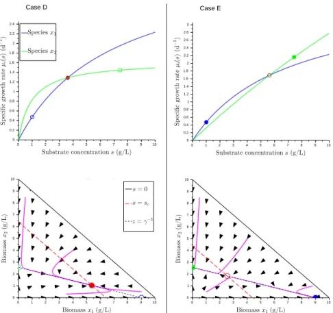
The asymptotic behavior of System (4) is illustrated on Figures 1 and 2 for the different cases. The control law is robust whenever all the stable equilibrium lead to a productivity greater or equal toP1 (see Table 1).
Restriction to more realistic cases. In order to restrict our analysis to a more realistic case, we consider a subset of S more relevant from an ecological point of view. We consider that each parameter represents a trait that is involved in the fitness of the species. A species with the best values for each trait will outcompete all the other species in any environmental conditions, and such super mutant should not exist. Actually, one may assume trade-offs between the different traits. For m traits, we consider that the m archetypes (or specialist, i.e. a species with the best value for one trait and the worst values for the others) define a Pareto front where all the species lie [Shoval et al. 2012]. In our example, we consider three archetypes xµ¯, xK, xα, with:
θµ¯= (¯µ+, K+, α−) θK = (¯µ−, K−, α−)
θα= (¯µ−, K+, α+)
Note that the best value for K is K−. These archetypes define the subset ¯S:
1 note that we ignore subsets of null measure corresponding to
non-generic cases, since they will never appear in practice (for example the cases s∗= sc, or s∗2= sc).
0 1 2 3 4 5 6 7 8 9 10 0 2 1 0.2 0.4 0.6 0.8 1.2 1.4 1.6 1.8 2.2 2.4 Case A 0 1 2 3 4 5 6 7 8 9 10 0 10 2 4 6 8 1 3 5 7 9 0 1 2 3 4 5 6 7 8 9 10 0 2 1 3 0.2 0.4 0.6 0.8 1.2 1.4 1.6 1.8 2.2 2.4 2.6 2.8 Case B 0 1 2 3 4 5 6 7 8 9 10 0 10 2 4 6 8 1 3 5 7 9 0 1 2 3 4 5 6 7 8 9 10 0 2 1 3 0.5 1.5 2.5 3.5 Case C 0 1 2 3 4 5 6 7 8 9 10 0 10 2 4 6 8 1 3 5 7 9
Fig. 1. Asymptotic behavior of System (4), Case A-C (see Proposition 5 and Table 1). Top: Specific growth rates as a function of substrate concentration. Bottom: Phase portraits with some trajectories (in purple). Filled circle: stable equilibrium, blank circles: unstable equilibrium. Blue: species x1, green: species x2, red: coexistence.
Table 1. Equilibrium and robustness for System (4) (see Proposition 5)
Case Conditions E0 Ew E1 E2 Ec Robustness
A ¬C1 LS uns - no - F
B C1.C4.(¬C5) uns uns GS uns no T
C C1.(¬C4).C5 uns uns uns GS no T iffP2= µ2(s∗2)(sin− s∗2)≥ P1
D C1.(¬C4).(¬C5)a uns uns uns uns GS T iffP
c= µ1(sc)(sin− sc)≥ P1
E C1.C4.C5b uns uns LS LS uns T iffP
2= µ2(s∗2)(sin− s∗2)≥ P1
LS: locally stable, GS:globally stable, uns: unstable, -:whatever, T/F: True/False. a: or equivalently C1.C2.C3.C6.
b: or equivalently C1.C2.C3.(¬C6).
¯
S :={θ = aθ¯µ+bθK+cθα, ∀(a, b, c) ∈ [0, 1]3| a+b+c = 1}
(14) Thus, for any triplet (ai, bi, ci)∈ [0, 1]3 | ai+ bi+ ci = 1,
the parameter vector of the species xi(ai, bi, ci) is given
by: θi = aiµ¯ ++ (1− a i)¯µ− biK−+ (1− bi)K+ ciα++ (1− ci)α− (15)
The morphospace, i.e. the space of trait values, is rep-resented on a ternary plot in Figure 3. Each vertex of the triangle represents an archetype. We consider Con-trol law (3) designed for a species x1(0.4, 0.3, 0.3) located
near the center of the morphospace. After discretizing the morphospace, we test for each additional species which conditions (C1, C4, C5) hold in order to determine the asymptotic behavior of the system (see Proposition 5 and Table 1). This allows us to define SR(represented in color
on Figure 3), a subset of ¯S, such that Control law (3) is
(SR, 1,P) robust.
First, one can see that the presence of an additional species can increase the productivity. On the other hand, the control law is not robust for a large subsets of ¯S,
cor-responding mainly to an additional species with a smaller yield coefficient than species x1(α2< α1). Two situations
may occur: the productivity at a stable equilibrium point (E2 or Ec) is smaller than the productivity P1, or there
is a reactor shutdown (s and y converge towards zero). A small decrease in productivity can actually be tolerated (although it is not considered in the present definition of multispecies robustness). On the other hand, the reactor shutdown is much more problematic and represents a real drawback of Control law (3). Anyway, parameter γ can be tuned in order to avoid as far as possible such situation, i.e. to increase the robustness to biodiversity of the control law.
The study of robustness for n species is obviously more delicate and is now under investigation.
0 1 2 3 4 5 6 7 8 9 10 0 2 1 0.2 0.4 0.6 0.8 1.2 1.4 1.6 1.8 2.2 2.4 Case D 0 1 2 3 4 5 6 7 8 9 10 0 10 2 4 6 8 1 3 5 7 9 0 1 2 3 4 5 6 7 8 9 10 0 2 1 3 0.2 0.4 0.6 0.8 1.2 1.4 1.6 1.8 2.2 2.4 2.6 2.8 Case E 0 1 2 3 4 5 6 7 8 9 10 0 10 2 4 6 8 1 3 5 7 9
Fig. 2. Asymptotic behavior of System (4), Case D-E (see Proposition 5 and Table 1). Same legend as Figure 1.
Fig. 3. Robustness of Control law (3) on a ternary plot of the morphospace ¯S. Each vertex represents an
archetype: x¯µ(1, 0, 0), xK(0, 1, 0), xα(0, 0, 1). The
di-amond represents species x1(0.4, 0.3, 0.3). The set of
species SR, such that Control law (3) is (SR, 1,P)
ro-bust, is represented in color. The color map represents the relative increase of productivity (with respect to
P1).
4. DISCUSSION
The robustness with respect to parametric uncertainty is classically studied for bioprocess control laws. Here, we
have defined the multispecies robustness. These two ap-proaches are clearly not equivalent. Actually, the n species can be seen as one species with time-varying kinetic and stoechiometric parameters. Such time-varying aspect is generally not considered in parametric uncertainty. More-over, the multispecies robustness also involves species com-petition/selection/coexistence. These phenomena, which affect bioprocess productivity, are not considered in the robustness with respect to parametric uncertainty.
4.1 Link with species competition
The classical theory of species competition [Smith and Waltman 1995] does not apply when the chemostat is operated with a closed loop control, and some surprises can arise. For example, if we consider a slow growing species
x2 (with µ2(s) < µ1(s), ∀s ∈ (0, sin)), we expect that this
species will rapidly be outcompeted (as it happens in open loop), so it should not affect the asymptotic behavior of the system. Actually, with Control law (3), the substrate depletion equilibrium E0 can become locally stable in
presence of x2 (if α2γsin < 1), so this species can cause
reactor shutdown (see Figure 1, Case A).
4.2 Coexistence of two species
The stable coexistence of two species is possible whenever their specific growth rates intersect. In open loop, this is not possible in practice since the dilution should be chosen exactly equal to the rate at which growth curves intersect. On the other hand, De Leenheer and Smith [2003] have proposed a feedback control for the stable coexistence of two species. Assuming increasing growth
rates and measurement of both biomass concentrations
x1 and x2, the feedback u = c1x1 + c2x2 + ϵ (where c1, c2, and ϵ are constant which should be chosen such
that some conditions hold) globally stabilizes the system towards a coexistence point. Gouz´e and Robledo [2005] have extended this approach for non-monotone growth rates with only the measurement of the sum of biomass concentrations x1+x2. In both studies, the original system
is gathered in a planar competitive system. This allows to exclude the existence of periodic solution using Poincar´ e-Bendixson Theorem. Here, we have shown that the feed-back law (3) can also lead to stable coexistence. In this case, we obtain a planar system which is not competitive (and neither cooperative). A change of coordinate (System (13)) is used to show the absence of periodic solution. To guarantee stable coexistence for two species with this control law, one must choose the set-point s∗accordingly. Assuming without loss of generality µ′1(sc) > µ′2(sc), the
coexistence point Ec is globally asymptotically stable iff
α1> α2 and 0 < s∗2 < sc < s∗ < sin. This last condition
is fulfilled whenever on choose s∗∈ (s∗, s∗), where
s∗= max{sc, sin(1− α2/α1)} ,
s∗= min{sin, sin(1− α2/α1) + sc} .
If α1 < α2, Control law (3) does not allow stable
coexis-tence.
4.3 Challenges
Maintaining a high bioreactor productivity despite inva-sive species (or new individuals resulting from natural mutations) turns out to be a challenging problem to en-sure process robustness. New questions arise now, such as detecting and preventing the apparition of ”bad species”. Observers could be set-up to early identify new compet-ing species with reduced productivity capability. Control strategies, such as extremum-seeking [Guay et al. 2004], could be adapted in order to consider multispecies and maintain conditions favorable for the settlement of mote productive species. As demonstrated in this paper, such control strategies could use this opportunity to continu-ously improve the reactor performance.
5. CONCLUSION
We have introduced the concept of multispecies robust-ness for bioprocess control laws. We have illustrated our approach with a control law proposed in Mailleret et al. [2004]. Depending on the characteristics of the additional species, some counter-intuitive results may appear such as coexistence, or even reactor shutdown when a slow-growing species is introduced. This framework should be used to design multispecies robust control laws and there-fore better tame biodiversity within a biotechnological process.
REFERENCES
Bastin, G. and Dochain, D. (1990). On-line estimation
and adaptive control of bioreactors. Elsevier, New York.
Bayen, T. and Mairet, F. (2014). Optimization of the sep-aration of two species in a chemostat. Automatica. doi: http://dx.doi.org/10.1016/j.automatica.2014.02.024. Available online.
De Leenheer, P. and Smith, H. (2003). Feedback control for chemostat models. Journal of Mathematical Biology, 46(1), 48–70.
Dochain, D. (2008). Automatic control of bioprocesses.
John Wiley & Sons, Inc.
Gajardo, P., Ramirez C., H., and Rapaport, A. (2008). Minimal time sequential batch reactors with bounded and impulse controls for one or more species. SIAM
Journal on Control and Optimization, 47(6), 2827–2856.
Gouz´e, J.L. and Robledo, G. (2005). Feedback control for nonmonotone competition models in the chemostat.
Nonlinear Analysis: Real World Applications, 6(4), 671–
690.
Guay, M., Dochain, D., and Perrier, M. (2004). Adaptive extremum seeking control of continuous stirred tank bioreactors with unknown growth kinetics. Automatica, 40(5), 881–888.
Karafyllis, I., Kravaris, C., Syrou, L., and Lyberatos, G. (2008). A vector lyapunov function characterization of input-to-state stability with application to robust global stabilization of the chemostat. European Journal of Control, 14(1), 47–61.
Mailleret, L., Bernard, O., and Steyer, J.P. (2004). Robust nonlinear adaptive control for bioreactors with unknown kinetics. Automatica, 40:8, 365–383.
Mairet, F., Mu˜noz-Tamayo, R., and Bernard, O. (2013). Driving species competition in a light-limited chemo-stat. In 9th IFAC Symposium on Nonlinear Control
Systems (NOLCOS).
Mazenc, F., Malisoff, M., and Harmand, J. (2008). Further results on stabilization of periodic trajectories for a chemostat with two species. IEEE Transactions on Automatic Control, 53, 66–74.
Perrier, M., de Azevedo, S.F., Ferreira, E., and Dochain, D. (2000). Tuning of observer-based estimators: theory and application to the on-line estimation of kinetic parameters. Control Engineering Practice, 8(4), 377– 388.
Ramirez, I., Volcke, E.I., Rajinikanth, R., and Steyer, J.P. (2009). Modeling microbial diversity in anaerobic digestion through an extended adm1 model. Water research, 43(11), 2787–2800.
Sbarciog, M. and Vande Wouwer, A. (2012). Some consid-erations about control of multi-species anaerobic diges-tion systems. In Proceedings of the 7th Vienna
Interna-tional Conference on Mathematical Modelling (MATH-MOD). Vienna, Austria.
Shoval, O., Sheftel, H., Shinar, G., Hart, Y., Ramote, O., Mayo, A., Dekel, E., Kavanagh, K., and Alon, U. (2012). Evolutionary trade-offs, pareto optimality, and the geometry of phenotype space. Science, 336(6085), 1157–1160.
Smith, H.L. and Waltman, P. (1995). The theory of the
chemostat: dynamics of microbial competition. Cam-bridge University Press.