Dynamic Scan Chains
A Novel Architecture to
Lower the Cost of VLSI Test
by
Nodari S. Sitchinava
Submitted to the Department of Electrical Engineering and Computer
Science
in partial fulfillment of the requirements for the degree of
Master of Engineering in Electrical Engineering and Computer Science
at the
MASSACHUSETTS INSTITUTE OF TECHNOLOGY
August 2003 L:/-Q¥¥'?z,;.,
'
:;;
() Nodari S. Sitchinava, MMIII. All rights reserved.
The author hereby grants to MIT permission to reproduce and
distribute publicly paper and electronic copies of this thesis document
in whole or in part.
A 1 / . MASSACHUSETTS OF TECHNOLJUL
2
0
LIBRAR
Author .. '.,, .....Department of Electrical Engineering and Computer Science
August 8, 2003
C ertified by ...
Rohit Kapur
Principal Engineer, Test Research and Development, Synopsys Inc.
/
Thesis Supervisor
Certified by ...
...
...
...
Daniel A. Spielman
Associate Professor
Thesis Supervisor
Accepted b ...
Arthur C. Smith
Chairman, Department Committee on Graduate Students
INST'ITUTF
_OGY
200
Dynamic Scan Chains - A Novel Architecture to Lower the
Cost of VLSI Test
by
Nodari S. Sitchinava
Submitted to the Department of Electrical Engineering and Computer Science on August 8, 2003, in partial fulfillment of the
requirements for the degree of
Master of Engineering in Electrical Engineering and Computer Science
Abstract
Fast developments in semiconductor industry have led to smaller and cheaper inte-grated circuit (IC) components. As the designs become larger and more complex, larger amount of test data is required to test them. This results in longer test appli-cation times, therefore, increasing cost of testing each chip. This thesis describes an architecture, named Dynamic Scan, that allows to reduce this cost by reducing the test data volume and, consequently, test application time.
The Dynamic Scan architecture partitions the scan chains of the IC design into several segments by a set of multiplexers. The multiplexers allow bypassing or includ-ing a particular segment durinclud-ing the test application on the automatic test equipment. The optimality criteria for partitioning scan chains into segments, as well as a parti-tioning algorithm based on this criteria are also introduced.
According to our experimental results Dynamic Scan provides almost a factor of five reduction in test data volume and test application time. More theoretical results reach as much as ten times the reductions compared to the classical scan methodologies.
Thesis Supervisor: Rohit Kapur
Title: Principal Engineer, Test Research and Development, Synopsys Inc. Thesis Supervisor: Daniel A. Spielman
Acknowledgments
The research for this thesis was conducted during my VI-A internships at Synop-sys, Inc. I take this opportunity to thank everyone who helped me by providing valuable advice, guidance and support during the entire research process.
First of all, I thank Professor Daniel Spielman for working with me and supervis-ing this thesis. His ideas were the basis for the optimization and algorithmic work presented here.
The initial idea behind Dynamic Scan architecture was proposed and patented by Rohit Kapur and Tom Williams from Synopsys. Rohit, who was my Synopsys thesis supervisor, was the driving force behind this project and his intelligence, en-couragement and enthusiasm made it easy and pleasant to work with him. Tom was one of the main promoters of this research. I thank him for the encouragement and constructive dialogs, which always brought new insights to the project. I would like to thank Jim Sproch, Director of Test Automation Products R&D Department, for all his support, as well as the opportunity to work at Synopsys. I also thank my manager Tony Taylor together with other managers Surya Duggirala, Girish Patankar and Wolfgang Meyer for their support and willingness to help whenever I needed their expertise in the area. Emil Gizdarski and Frederic Neuveux were on the Dynamic Scan project team and provided invaluable suggestions about the new architecture as well as help with modifying Synopsys tools to suit the architecture. I thank Sudipta Gupta, Nahmsuk Oh and many others at Synopsys for their readiness to give assis-tance whenever I needed it. Last but not least I thank Minesh Amin, to whom I owe most of my limited knowledge of ATPG, and Samitha Samaranayake, my friend and fellow VI-A intern, for their constructive suggestions and discussions on the topic, as well as indispensable contributions which made this project a success.
I thank Gergana Bounova for extensive comments on the manuscript and help editing this thesis.
Finally, I would like to thank my parents for all their support and the sacrifices they have made for me throughout the years.
Contents
1 Introduction
1.1 Testing Integrated Circuits .
1.2 Motivation for Low-Cost VLSI Test Methodologies ... 1.3 Prior Work.
1.4 Our Contributions ... 1.5 Structure of the Thesis ...
2 Introduction to Structural IC Testing
2.1 Fault Models ...
2.2 ATPG for Combinational Circuits ... 2.3 Testing Circuits with Sequential Elements ...
3 Dynamic Scan Architecture
3.1 Motivation for Dynamic Scan ...
3.2 Single Scan Chain Dynamic Scan Design ... 3.2.1 Using Segments.
3.3 Dynamic Scan with Multiple Scan Chains ...
4 Segment; Partitioning
4.1 Notation.
4.2 Dynamic Scan Objective Function ... 4.3 The Partitioning Algorithm ...
4.3.1 Complexity Analysis of the Algorithm ...
13 13 15 15 19 20 21 22 23 25 29 29 31 33 34 37 37 38 39 40
4.3.2 Improving the Runtime ... 42
4.4 Discussion ... 43
5 The Results 47
5.1 Experimental Setup ... 47
5.2 Test Application Time as a Function of the Number of Partitions . 48
6 Conclusions and Future Research 51
6.1 Conclusions ... 51
6.2 Future Research ... 52
A Design Specifications 55
B Additional ATPG Information 57
C Scan Flip-Flop Usage 59
List of Figures
1-1 Trend of the cost of manufacturing and testing ASIC designs ... 16
2-1 A sample design and a corresponding test vector ... 24
2-2 Scan flip-flop design ... 26
3-1 A sample IC with a single scan chain ... 30
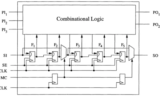
3-2 An extreme case of Dynamic Scan architecture with a multiplexer in front of each scan flip-flop ... 32
3-3 Using segments for Dynamic Scan ... . 34
3-4 Dynamic Scan for multiple scan chain designs ... 35
4-1 A sample set of partitioned test vectors and the corresponding values 38 4-2 Pseudocode for the BASIC-PARTITION algorithm ... 41
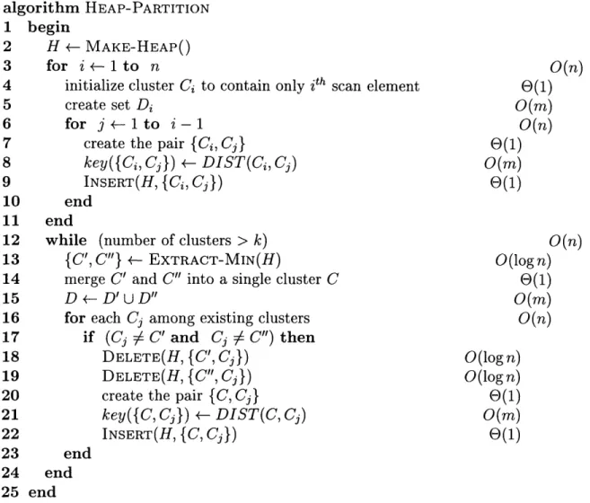
4-3 Pseudocode for the HEAP-PARTITION algorithm ... 44
5-1 Trend of test application time reduction as a function of the number of segments . . . 49
List of Tables
3.1 A sample set of test vectors before random fill ... 30 3.2 Use of the scan elements during dynamic scan for the sample set of
test vectors ... 32
4.1 The result of running BASIC-PARTITION algorithm on a sample set of
test vectors ... 41
5.1 Reduction in test application time using Dynamic Scan over regular scan 50 A.1 ISCAS '89 benchmark design specifications ... 55 A.2 Industrial circuits design specifications ... 55 B.1 Additional ATPG information ... 57
Chapter 1
Introduction
Rapid developments in semiconductor industry have led to smaller and cheaper inte-grated circuit (IC) components. As a result, a single design can accommodate more units. The increase in the number of the IC components in the designs increases the design complexity and, consequently, the cost of VLSI testing. This thesis describes an architecture that helps reduce this cost.
1.1
Testing Integrated Circuits
This thesis focuses on the structural test of integrated circuits. Structural test assumes that the design is implemented according to its specifications and checks if any defects have been introduced during the fabrication process of the chip [2].
This section introduces the basic ideas behind the structural test. More rigorous discussion of IC testing is provided in Chapter 2.
A fabricated IC is placed on Automatic Test Equipment (ATE, or tester) which supplies a set of binary vectors, called test vectors or test patterns, to the input pins of the chip. The test vectors have been predetermined using automatic test pattern generation (ATPG) techniques based on the design specifications of the chip. The vectors specify a set of input values for the design as well as corresponding outputs of
1Verification, a process conducted on the design prior to fabrication, checks if the implementation behaves according to the specifications.
a defect-free design. The ATE propagates the inputs specified by the vector through the fabricated chip and observes the values on the output pins of the chip. The observed output values are compared against the ones specified by the test vectors and if at least one of the observed values differs from the specified ones, the chip is declared defective. The probability that the chips that pass all the test vectors are indeed not defective (i.e.there are no false positives) depends on the exhaustiveness of the test and is called test coverage.
As designs become more complex it becomes more difficult to achieve high test coverage. Test engineers add additional hardware to the design to alleviate the com-plexity of test pattern generation and to increase the test coverage. Such hardware addition for purely testing purposes is call Design for Testability (DFT) and has been widely accepted to improve test coverage [2].
Sequential elements, such as flip-flops, create additional logic states for the circuit. This increases ATPG complexity making it harder to achieve high test coverage. Scan
design, one of the most commonly used DFT methodologies for testing sequential
designs, reduces the ATPG complexity by providing implicit control and observability of the flip-flop states [2]. This is achieved by adding a test mode to the design such that when the circuit is in that mode, all flip-flops are interconnected into chains and act as shift registers. In the test mode, the flip-flops2 can be set to an arbitrary state by shifting those logic states through the shift register. Similarly, the states can be observed by shifting the contents of the shift registers out. Thus, the inputs and outputs of the flip-flops act almost like primary inputs and primary outputs of the design and the combinational logic between the flip-flops can be tested with the simpler methods used for purely combinational circuits.
2The modified flip-flops are also called scan flip-flops, scan elements or scan cells. Similarly, the
1.2
Motivation for Low-Cost VLSI Test
Method-ologies
The cost of testing an IC depends on many factors, among which the price of the testers is of major concern. Today, the price of a single ATE unit can reach as much as $3.5 million [29]. The efficient use of the testing equipment is, therefore, essential in keeping the cost of test low.
As the designs become larger and more complex, larger volumes of test data3 are required to test them. This results in longer test application times - time each chip needs to spend on the tester - therefore, increasing the testing cost of each chip.
Furthermore, cost problems arise when the test data volume exceeds the total ATE memory where the test vectors are loaded. Upgrading testers every time a new larger design is produced can significantly escalate the cost of the test.
Thus, efficient use of testers as well as tester reusability are essential for cost-effective VLSI test.
As seen from Figure 1-1, the per transistor cost of manufacturing integrated cir-cuits has been falling steadily in the past 20 years, while the cost of testing has remained relatively the same. This means that the cost of testing an IC has been rising relative to the total cost of the complete designs. The International Technol-ogy Roadmap for Semiconductors predicted that the cost of testing ICs may surpass the cost of manufacturing them by 2014 unless new low-cost methodologies are not developed [28].
1.3
Prior Work
The increasing cost of testing integrated circuit relative to the total design and man-ufacturing cost has spawned much research into creating low-cost test strategies. As the designs become more complex, the test application time is dominated by the time it takes to shift the values in and out of the scan chains. This is due to the fact
3
0.01 0.001 0.0001 o le-05 v: le-06 le-07 1 noQ 1980 1985 1990 1995 2000 2005 2010 2015 Year
Figure 1-1: Trend of the cost of manufacturing and testing ASIC designs on per transistor basis [28].
that the test data can be applied and observed at the primary input/output pins in one clock cycle. On the other hand, to apply and observe values at the
pseudo-input/output pins, as the scan flip-flops are usually called, it might take the number
of clock cycles up to the length of the longest scan chain because the values have to be shifted sequentially through a single scan-in and a single scan-out pins. Thus, most efforts to reduce the cost of test are directed toward reducing the test data volume and test application time by shortening and rearranging scan-chains or by complete modification of the DFT approach. Some of these low cost test solutions are presented below.
In partial scan method, only some of the flip-flops are converted into scan flip-flops. A variety of hybrid test generation schemes, using both scan based and sequential ATPG, have been proposed to reduce test application time [17, 22, 25]. Since these schemes are not full scan, multiple clock cycles are required to propagate a value from the (pseudo-)inputs to the (pseudo-)outputs. The number of clock cycles required depends on the longest sequential path in the test. The test vector generation for large sequential circuits is complicated and time consuming. Therefore, these hybrid
Cost of manufacturing a transistor
Cost of testing a transistor 0
-test schemes do not scale well and cannot be used with large sequential designs. There is no evidence of the hybrid test methods being tested on any circuits with more than three thousand gates [17, 22, 25].
A different proposed strategy is to create multiple scan chains [22, 20] and load them in parallel using one input per scan chain. Thus the length of the longest scan chain is reduced which decreases the test application time. However, loading a large number of scan chains in parallel requires many input and output pins on the chip, which can be impractical because the number of I/O pins is physically limited by the size of the chip, as well as by the number of pins on the tester. Therefore, the number of available pins limits the parallelism that can be achieved. Furthermore, in both of the above schemes, gains are limited to test application time while test data volume is not addressed.
In Partial Parallel Scan [16], the architecture allows for groups of flips-flops to be changed from scan flip-flops to non-scan flip-flops during the test process. The test engineer can switch between different levels of partial scan and save the time and data spent on loading unnecessary scan cells. However, this switching architecture requires complex control logic with high hardware overhead. Partial Parallel Scan is able to reduce test application time by one to two orders of magnitude [16]. Despite the satisfactory results, this is still not a full scan technique: the test generation process becomes much harder for the ATPG engine and results in lower test coverage. In addition, even though partial scan is used to minimize the hardware overhead, the extra 6%-19% area overhead of this DFT architecture [16] is large, and therefore impractical to use in many designs. Partial Parallel Scan also addresses only the reduction of test application time while leaving the test data volume unchanged.
Built-in Self-Test (BIST) techniques use Linear Feedback Shift Registers (LFSR)
to generate the test patterns [2]. These LFSRs are built around the circuit so that an ATE is not needed to apply these test vectors. The test data volume is significantly reduced since most of the data no longer needs to be fed into the chip. The test vectors created by a LFSR are pseudo-random sequences of binary values based on an input seed given to the LFSR. These vectors are not created by targeting faults in the
circuit like an ATPG engine does. Therefore, the on-chip test depends on the random detection of faults and is much less efficient than the test vectors created by an ATPG engine. Due to this inefficiency, the number of test vectors increases by as much as ten times and increases the test application time [1]. The most significant gains in test application time have been shown using Logic BIST (LBIST) [32, 4, 10, 15] and
deterministic BIST (DBIST) [24, 8, 5], both of which are hybrid schemes between
ATPG and BIST. However, these schemes come at a significant hardware overhead of 13% to 20% [28] and require certain modifications to the non-DFT elements of the circuit. These modifications can be intrusive to the functionality of the circuit and might not even be possible in certain designs. Even though such drawbacks exist, BIST based test methods are still very popular, since the use of expensive ATE time is avoided in these methods.
Illinois Scan architecture [9] suggests another solution to the low cost test problem.
In Illinois Scan, a large number of scan chains are grouped into a few scan groups and loaded in parallel using one input pin per scan group. Illinois Scan consists of two operating modes. The first one, known as the broadcast mode, connects each group of scan chains to one input pin. Thus, a single test vector can be broadcast to all the scan chains that are connected in parallel. However, by connecting many chains to one input, new dependencies are added to the system: any two scan cells in the same position of different scan chains in the same group will always have the same value. Therefore, certain tests that require different values in the same position of the scan chains cannot be applied to the circuit. To solve this problem a second mode called
serial mode is maintained. In this mode, all the scan cells are connected together as
one long scan chain. This architecture performs well, as long as a large percentage of the vectors can be run in broadcast mode, since serial mode patterns are equivalent to regular scan testing. However, as the number of scan chains loaded in parallel, known as the parallelism, is increased, the number of dependencies in broadcast mode increases. This causes reduction in broadcast mode fault detection, which in turn increases the number of serial mode vectors. Therefore, this architecture is limited by the inability to detect most faults in broadcast mode when a large number of scan
chains are loaded in parallel.
Reconfigurable Shared Scan-in architecture (RSSA) [26], a recently proposed
vari-ation of Illinois Scan, manages to avoid the serial mode by defining several scan chain compatibility groups and using several scan-in pins. The compatibility groups define scan chains that are unlikely to conflict in the broadcast mode if they are connected to the same input pin. If a conflict does happen while detecting a particular fault, the group membership of the scan chains is dynamically modified and the fault is detected by reconnecting the conflicting scan chains to a different scan-in pin. RSSA provides excellent test data volume and test application time reductions. However, to determine the compatibility groups, the architecture utilizes iterative ATPG runs and takes very long time for large designs. In addition, significant modification are required for the ATPG engines.
1.4
Our Contributions
The architecture described in this thesis reduces test application time, as well as the test data volume with minimal addition of DFT and minimal modification to the ATPG. It was named Dynamic Scan Chains because it allows to dynamically reconfigure the scan chains during the testing mode.
Dynamic Scan was motivated by a previously proposed architecture which used subsections of a single scan chain architecture to apply tests to different design mod-ules [18, 19]. However, for that strategy to be effective, these modmod-ules must be well bounded and have independent test patterns, characteristics not found in current increasingly complex designs.
Dynamic Scan expands previously defined concepts for single scan chains to pro-vide a new architecture for use in conjunction with ATPG. The test patterns are applied to arbitrary logic, but the shortest possible scan chains are used for each pettern. To do so, the benefits of using multiple scan chains [20] are blended with the reconfiguration method for single scan chains. These methods work together to reduce test data volume and application time.
The technology is intended for use with already existing ATPG engines and the patterns produced by them. Thus, the solution avoids breaking the basic concept employed by today's scan chain construction methods: multiple scan chains that are active at any given time have a single path between the scan-ins and scan-outs of each scan chain. This distinguishes Dynamic Scan architecture from more radical solutions that fan out scan chains from a single scan-input [9].
The benefits of the Dynamic Scan depend on the way scan chains are divided into segments. This thesis introduces the optimality condition to maximize the benefits of the Dynamic Scan, as well as a partitioning algorithm that divides the scan chains into segments.
During the course of our investigations we have prototyped the architecture, con-ducted experiments and collected data for ISCAS '89 benchmark designs [12] as well as larger designs currently used in industry.
A patent for Dynamic Scan architecture has been filed with the US Patent and Trademark Office and is pending for approval [14].
1.5
Structure of the Thesis
In Chapter 2 the concepts involved in VLSI testing are presented more rigorously. In Chapter 3 Dynamic Scan architecture is described. Chapter 4 is devoted to the partitioning algorithm which maximizes the benefits of the Dynamic Scan. Chapter 5 presents the results of the simulations. Finally, Chapter 6 summarizes the thesis conclusions and suggests ideas for future research.
Chapter 2
Introduction to Structural IC
Testing
To test a fabricated IC, the chip is placed on an Automatic Test Equipment (ATE or tester) which supplies a set of binary vectors, called test vectors or test patterns to the input pins of the chip. The test vectors have been predetermined based on the design specifications of the chip. These vectors specify a set of input values for the design as well as corresponding outputs of a defect-free design.
After the vectors are applied the clock is pulsed and the values are propagated from the inputs of the chip to its outputs. The ATE compares the actual output values of the chip to the ones specified by the test vectors and if at least one of them differs, the chip is declared defective. However, if a chip passes all the test vectors the probability that it is indeed not defective (i.e. is not a false positive) depends on the exhaustiveness of the test and is called test coverage.
One way to produce a set of patterns that will result in high confidence test is by defining them as a set of all possible inputs to the chip. However, the number of all possible patterns grows exponentially with the number of input pins on the chip1. Given that there are thousands of pins on a typical chip [28], this method is not practical. In fact, a much smaller set of patterns is usually produced to achieve
1For designs with sequential elements, like flip-flops, the number of all possible patterns grows
confidence levels as high as 95%-100%. The process of finding the effective set of test patterns is called automatic test pattern generation (ATPG) and is one of the key tasks in IC test automation [23].
As designs become more complex it becomes more difficult to achieve high test coverage using reasonable resources. Test engineers add additional hardware (DFT) to the design to alleviate the complexity of test pattern generation and to increase the test coverage.
This chapter covers the basics of ATPG and DFT required for understanding Dynamic Scan architecture. For more comprehensive coverage the reader is refered to the book by Bushnell and Agrawal [2].
2.1
Fault Models
For testing purposes, the possible defects that can occur during the manufacturing process of the chip are abstracted by several fault models [1, 2]. The most commonly used fault model is single stuck-at fault model, which in practice captures over 95% of all possible manufacturing defects [3]. In this model the circuit is modeled by the collection of interconnected logic gates (called a netlist). Each interconnection
might have two type of stuck-at faults - stuck-at-0 (s-a-O) or stuck-at-1 (s-a-1). The stuck-at-0 fault models a conducting path, a short, from the connection to logic "ground", i.e. the connection will always have a logic value 0 regardless of the actual value being driven through it. Similarly, if the connection has a stuck-at-1 fault, then there is a conducting path from it to the power supply and the connection will always have a logic value 1. The faults are modeled by creating a fault list - a list of all potential stuck-at faults [1]. Since there are two type of stuck-at faults for each interconnection, a circuit with n interconnections will have a fault list of size 2n. Test
coverage, the quality metric for the exhaustiveness of the test, is the percentage of
faults from the fault list that will be detected by the test vectors. The automatic test pattern generation engine uses the fault lists to create test vectors that will detect these faults.
2.2
ArPG for Combinational Circuits
In this section we restrict ourselves only to circuits that do not have any sequential elements (flip-flops or latches). Section 2.3 discusses how introduction of sequential
elements to the designs affect the test methodologies.
The output of the ATPG engine is a list of test vectors. A test vector (sometimes also called a test pattern) is a binary vector where each entry corresponds to a par-ticular input or output pin of the chip. The test vectors specify a set of input values for the design as well as corresponding outputs of a defect-free design. Thus if the input entries of the test vector are applied to the ICs input pins, the output pins of the defect-free chips will have the same values as specified by the test vectors' output entries. The tester compares the actual output values of each IC to the ones defined by the test vectors. If at least one vector output value differs from the observed ones, the chip is defective.
To generate the test vectors the ATPG engine initializes a vector to undefined values. They are usually called don't cares or X's 2. As the pattern is formed, the undefined values are filled with binary values 0 or 1.
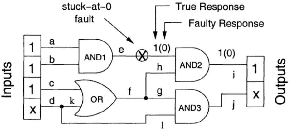
After the patterns have been initialized, the ATPG engine picks a fault from the fault list and fills in the vector with the values that can sensitize the fault. For example, consider the netlist in Figure 2-1. To sensitize the stuck-at-0 fault at the e interconnection, we need to set the inputs a = 1 and b = 1. Then the output of the AND1 gate in a non-defective chip would output 1 while in the faulty chip it would output 0. Therefore, the first two input entries of the test vector would be set to l's. Having sensitized a fault, the ATPG engine needs to propagate it to the output pins where it can be observed. In the same example, to propagate the faulty response to the output pins, the connection h needs to be set to 1. This can be achieved by setting one of the inputs c or d to 1, which forces the OR gate to output 1 3. As for the output entries of the vector, entry i is set to the true response of a defect-free
2
The name "X" is commonly used because value 'x' is assigned to the currently undefined vector entries in most ATPG implementations.
30nly one of the inputs to the OR gate needs to be specified, while the other input can be left uninitialized.
stuck-at-0 True Response C/, -a C a C. :3 I
Figure 2-1: A sample design and a corresponding test vector. The pattern will detect the stuck-at-0 fault at the output of the ANDI gate. 'x' within the pattern denotes
don't care values.
circuit, while the output j is left uninitialized since it depends on the value of input d. Thus, the test vector with the input entries 11x and the output entries lx will detect the stuck-at-0 fault on interconnection e.
To minimize the number of patterns required, the ATPG engine picks another fault from the fault list and tries to set the appropriate bits of the same test vector. This might not be always possible, because distinct values might need to be set in the same entry of the test vector. For example, in Figure 2-1 it is impossible to test both stuck-at-0 and stuck-at-1 faults on the e interconnect. Finding the minimal set of test vectors is found to be NP-Complete [11], therefore, the efficient engines use heuristics in choosing which faults to pack into which vectors.
After ATPG stops filling in a particular vector, the input vector bits that haven't been defined yet, are filled with random values. Then the fault simulation engine propagates all the inputs of the test vector through the circuit to the circuit outputs and all the undefined output bits of the test vector are set to the propagated values. There are two main reasons for filling the remaining x's with random values. First, the ATE equipment recognizes only binary values and does not understand the concept of don't care values. This reduces the price of already expensive tester equipment. The second reason for filling x's with random values is due to the sub-optimality of the ATPG heuristics there might be more faults that could have been detected by the same vector. Filling the x's with random bits, allows for random detection of
such faults. The number of such randomly detected faults is high for the first few test vectors. However, it reduces significantly after first couple of hundred vectors and there are many of don't care values filled with random bits that are not used for detecting any faults [27]. As it will be described in Chapter 3, the Dynamic Scan architecture reduces test data volume by providing the flexibility not to load the tester with such unused bits of the vectors at all.
2.3
Testing Circuits with Sequential Elements
Sequential elements, such as flip-flops, create additional complexity to structural test because they are able to temporarily store logic states of the circuit. Thus, the logic values of any part of the design depend not only on the current state, but also on the previous states stored and propagated through the flip-flops over time. Due to the increased complexity of the test pattern generation in the sequential designs the test coverage cannot be achieved as high as in purely combinational designs. This forced test engineers to look for new DFT methodologies to reduce the complexity of test pattern generation.
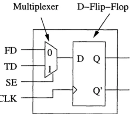
One of the most commonly used DFT techniques incorporates scan design [2]. It reduces the complexity of ATPG for sequential designs by providing direct access to the flip-flops. This is achieved by placing a multiplexer in front of each flip-flop, either as a separate element [1] or embedded into the design of the latch [6, 31]. An example of a modified flip-flop (also called scan flip-flop (SFF) or scan cell) is shown in Figure 2-2. All scan flip-flops in the design are interconnected into chains forming shift registers, also called scan chains.
Each SFF; has two modes- functional mode and scan mode. In the functional
mode the SFF acts as a normal flip-flop. In the scan mode, which is activated through the scan enable pin of SFF, the chain of flip-flops acts like shift registers. Thus, in the scan mode, each SFF can be set to an arbitrary state by shifting those logic states through the shift register. Similarly, the states can be observed by shifting the contents of the shift registers out. This way the inputs and outputs of the
flip-Multiplexer D-Flip-Flop
FD TD SE CLK
Figure 2-2: Scan flip-flop design. If Scan Enable (SE) signal is present, the flip-flop is in the test mode and the test data (TD) can be loaded. When SE signal is absent, scan cell operates like a regular flip-flop and functional data (FD) can be loaded on the flip-flop.
flops act almost like primary inputs and primary outputs of the design. Thus, the combinational logic between the flip-flops can be tested using the methods for purely combinational circuits.
The test application process on the ATE looks as follows:
1. Set the scan flip-flops in the test mode and shift the test vector onto them. 2. Apply the vector values to the primary inputs of the design.
3. Pulse the clock to capture the values propagated through the design.
4. Shift the values out from the flip-flops and measure the values on the output pins.
5. Compare the captured values to the ones specified by the test vector. If any of them differs, discard the chip as defective; else, repeat the process with the next vector.
As a simple example in Chapter 3 shows, shifting the values in and out of the scan flip-flops dominates the test application time. In contrast, the values on the primary input pins can be applied in one clock cycle and observed on the primary output pins in the same clock cycle when the values are available. For the scan flip-flops (also known as pseudo-inputs/outputs) the time it takes to load and observe all the
values is equal to the length of the longest scan chain. Theoretically, it can take up to two times the length of the longest scan chain to load values, propagate them to the pseudo-outputs, and unload (observe) them. However, in practice, loading and unloading is completed simultaneously - while the test data is loaded for the next test vector, the output data from the previous test vector is unloaded.
Chapter 3
Dynamic Scan Architecture
Over 90% of test data volume in the patterns are the randomly filled x's [27]. It has been observed that not all of the randomly filled values are useful in detecting the faults. However, modern testers do not support the notion of X's and, therefore, a lot of unused information that takes up useful resources during testing must still be defined in the test patterns. Dynamic Scan provides the ability to avoid specifying the unnecessary bits of the test vectors with minimal hardware and ATPG overhead and without any modification to the current ATE equipment.
3.1
Motivation for Dynamic Scan
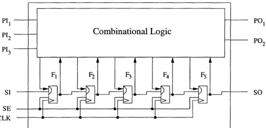
Consider a sample circuit presented in Figure 3-1. The design consists of the com-binational circuitry with three primary input pins (PI1, PI2, PI3 ) and two primary
output pins (PO1, P02), as well as five scan flip-flops (Fl, ... , F5) interconnected
into a single scan chain. The scan-in (SI) and the scan-out (SO) pins are used to load and unload the test vectors on the scan flip-flops; the scan enable pin (SE) configures the flip-flops for scan operations; the clock (CLK) synchronizes the whole circuit.
Table 3.1 presents a sample set of test vectors before the don't care entries are filled with random values. The tester applies the stimuli to the corresponding pins of the IC and observes the response on pins PO1, P0 2 and each of the scan flip-flop through SO pin as has been discussed in Chapter 2.
PO PI3 SI SE CLK PO2 SO
Figure 3-1: A sample IC with a single scan chain. The scan chain consists of five scan elements.
Let us calculate the time it takes to apply all the test vectors to the IC, the test
application time (TAT). As discussed above, test vectors are applied in the following
sequence:
1. Scan in vector Vi;
2. Stimulate inputs, measure outputs; 3. Pulse a capture clock;
4. Scan out vector Vi, simultaneously scan in the next vector Vi+l.
A tester first scans the data into the flip-flops, applies a stimulus to the inputs, and measures the circuit outputs. It then applies a pulse on the clock signals. The
Table 3.1: A sample set of test vectors before random fill.
Test Vectors Stimulus Response
(PI[1...3] F[1..5]) (PI[...2] F[1..5]) Vl11x xx1x x xxlxx V2 xOx xxOll 10 xxxxl V3 0 1 x xx100 xx Oxxlx V4 lxO x110 1 1 lx0xx PI,
pulse triggers an update of the scan chain flip-flops and thus captures the circuit's response to the test vector. The tester then scans out the response. At this point, the next test vector is simultaneously scanned in.
For the fixed configuration in Figure 3-1, the test vectors would operate the scan chain of length five. This scan operation dominates the test application time, taking five clock periods in the example scenario. Every test applying a stimulus to or measuring a response from the scan flip-flops would perform this scan operation and consume these five clock periods.
Each test vector in the example uses the scan elements; total test time per vector is 5 cycles for scan-in of vector Vi and scan out of vector Vi_1 plus 1 cycle for updating the flip-flops and 5 cycles for the scan out operation of the last test vector which could not be overlapped with other tests. Running the entire test of four vectors consumes (5 + 1) x 4 + 5 = 29 cycles. From this, the scan time is 25 clock cycles. The scan operation's duration is independent of the number of scan values the test needs. The rigid configuration presented in Figure 3-1 requires that the tester loads every scan flip-flop, that is why typical ATPG algorithms would randomly fill the don't cares and provide fully specified test vectors, i.e. the vectors that contain no x's .
3.2
Single Scan Chain Dynamic Scan Design
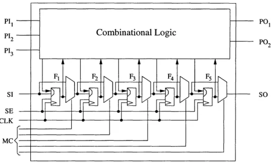
To use the test resources in the most efficient manner, the scan chains should ideally provide access to the flip-flops that the tests need. Figure 3-2 shows the scan chain structure that would allow this access. By setting the appropriate multiplexer control signals (MC), the configuration in Figure 3-2 can include or exclude any flip-flop from the scan chain, tailoring the scan chain to suit the test vector.
Signals that control the multiplexers let each flip-flop either be bypassed or in-cluded in the scan chain. The multiplexer control signals can be controlled from the circuit input pins (as presented in Figure 3-2), through a shift register configuration
(as shown later in Figure 3-3) or any combination of the two.
PI1 PI2 PI3 SI SE CLK MC PO PO2 SO
Figure 3-2: An extreme case of Dynamic Scan architecture with a multiplexer in front of each scan flip-flop.
test application time. In particular, using a shift register to control the multiplexers implies that time linear to the width of the shift register must be spent on the ATE to load the control bits before the test vectors are loaded. This increases the time to test each chip. Therefore, the design engineer must decide on the trade off suitable for a particular design depending on the number of pins available and test application time reduction she wants to achieve.
Table 3.2 lists the example test results for the architecture presented in Figure 3-2. A dash "-" signifies a value that was omitted from the test pattern by using a scan chain configuration that bypassed the associated flip-flop. Thus, considering the
Table 3.2: Use of the scan elements during dynamic scan for the sample set of test vectors.
Test Vectors Stimulus Response
(PI[1...3] F[1..5]) (PI[1...2] F[1..5])
VI l11x -- 10- xO -- lxx
V2 x0x -- 011 10 -- xxl
V3 0 1 X -- 100 xx Oxxlx
1-0--scan-ins of a test and the scan-outs of the previous test that occur at the same time, test vector V1 uses scan cells F3 and F4; tests V2 and V3 use scan cells F3, F4, and
F5; test V4 uses all scan cells F1, F2, F3, F4, and F5. The total scan time for all test
vectors is 2 + 3 + 3 + 5 + 2 = 15 cycles (because we take advantage of the overlapping scan-ins and[ scan-outs), which is much less than the total scan time of 25 cycles for the original scan chain.
This is a very expensive configuration in terms of supplying the multiplexer control signals. It would require many inputs to control the multiplexers; using a control register, on the other hand, would require loading the register for every test vector. Accounting for all these considerations the design might be impractical in an actual circuit layout. The next section describes a more realistic approach which limits the number of control signals by reducing the number of required multiplexers and by making multiple patterns use a single configuration.
3.2.1
Using Segments
For dynamic scan to be useful, segments should be created to limit the number of supported configurations. Segments are contiguous scan chain components that a scan test must bypass or use as a set. The benefits that dynamic scan could provide depend on the way the segments are identified.
Figure 3-3 shows an example of a dynamic scan configuration that uses segments. This configuration accounts for the fact that all the patterns in the example set use the last three scan cells.
Preventing test patterns from excluding individual scan cells offers a simpler so-lution compared to the one proposed in the previous section. However, it does not offer as large a reduction in test data volume and application time. In the above example, the scan segments force pattern V1 to use the F5 scan cell. In this case,
ATPG can randomly fill the don't care for F5 in this test pattern. The dynamic scan
chain implementations shown in Figure 3-3 provide an overall scan test application time (and proportional test data volume) of 3 + 3 + 3 + 5 + 5 = 19 cycles.
PI1 PI 2 PI3 SI -SE CLK MC CLK F1 F2 F3 F4 PO1 PO2 - SO2 .-
Figure 3-3: Using segments for Dynamic Scan.
bypass every scan element. That is, segment length equals 1. This configuration is most flexible and provides maximum benefits at the expense of design-for-test and layout problems. At the other extreme, a test does not bypass any scan cell, and the original scan chain is the only configuration available to the test patterns. This least flexible configuration does not effectively reduce test data volume or test application time, but it has minimal additional impact on the typical scan chain layout problems. Our goal falls in between these two extremes: we seek to achieve significant benefits with a small number of segments.
3.3
Dynamic Scan with Multiple Scan Chains
Dynamic Scan can easily be extended to designs with multiple scan chains. However, applying this to every chain independently would create significant overhead problems in test data volume. For this reason, the most promising concept in making dynamic scan a reality is to use the same control signal for the same segment over all scan chains.
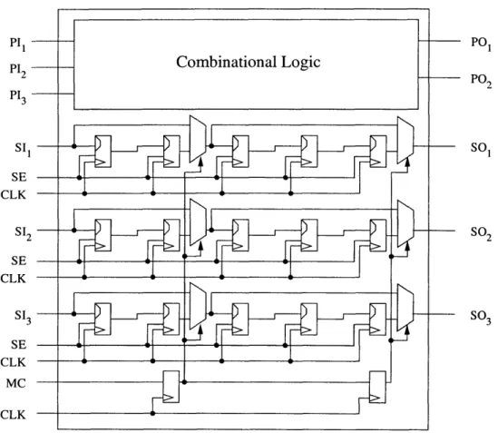
Figure 3-4 explains the concept graphically. In this example, all three scan chains are partitioned into the same number of segments (two). Each scan chain has the
34 Combinational Logic
.
_
FF"-
FF -'--
j -
FF->]---- i
-I
-I
I
I
-F!
---- F
>
-PI1 PI2 PI3 SI1 SE CLK SI2 SE CLK SI3 SE CLK MC CLK PO PO2 SO1 SO2 SO3
Figure 3-4: Dynamic Scan for multiple scan chain designs.
same number of scan flip-flops in a particular segment - two for the left segment and three for the right one. The same multiplexer control signals feed all three scan chains.
In addition to reducing the data volume required for multiplexer controls, this ap-proach allows for added flexibility when placing the scan flip-flops in the design. To allow the placement tools more flexibility, the algorithm that partitions scan chains into segments does not concern itself with the membership of scan elements to par-ticular scan chains, but only with groups of segments. Thus, for the above example the partitioning algorithm's output would state that the left six flip-flops belong to one partition, while the other nine flip-flops belong to the other partition. Thus, the placement tools have the freedom to rearrange the scan flip-flops across all the chains within a partition. This flexibility feature of Dynamic Scan becomes very important feature when placement and routing constraints are very tight.
Chapter 4
Segment Partitioning
The benefits of the Dynamic Scan depend on the way the scan chains are broken down into segments. In this chapter the optimality conditions for maximal Dynamic Scan benefits are defined. In addition, segment identification algorithm and its analysis are presented in Section 4.3
4.1
Notation
This section presents the notation that is used throughout this chapter.
SE - the set of all scan elements in the design
n - the number of scan elements in the design, i.e. SEI= n
Vi - the ith test vector
m - the number of test vectors for the design, i.e. m = max i
vi - the set of scan elements with non-X values in the ith vector
k the total number of segments we are trying to create
Cj - the set of scan elements placed in the jth cluster/segment
Dj - the set of test vectors that require the jth cluster/segment, that is, Dj = {vilvi n Cj 0}
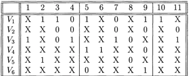
An example of a sample set of randomly partitioned test vectors and corresponding values for the variables are presented in Figure 4-1.
= {1,2,3,4,5,6,7,8,9,10,11} n = 11 V1 = [X 11O1XOXllX], m = 6 V2= [ X X 0 0 X X 0 X 0 X 0], etc. vl = {2,3,4,1,7,9, 10}, 2 = {3,4,7,9,11}, etc k = 3 C1 = {1,2,3,4), C2 = {5,6,7,8,9}, C3 = {10,11} D1 = {v1,V2,V 3, v5}, D2 = {V 1,V2, V3,V4, V5, V6}, D3 = {V1,V, 2 V3}
Figure 4-1: A sample set of partitioned test vectors and the corresponding values.
4.2
Dynamic Scan Objective Function
To determine the optimal partitioning for Dynamic Scan we must notice the following fact:
Observation: In a particular test vector, if at least a single scan flip-flop
within the segment is required for testing, then all the scan elements of the segment have to be loaded.
Taking the above observation into account we can define the optimization problem for Dynamic Scan as follows:
Problem: Determine the distribution of the set of scan cells SC into k
clusters Cj while minimizing the following function T(k):
Min T(k) = m i=1 j:vinCjA0
Cjl
(4.1) subject to, 381 2 3 4 5 6 7 8
9110 11
11
V
1,
1 1 0 1 XOX
1 X
V
2XXOOXXOXOX
0
V
3iXO
lxxilox
1
V3 1 X 0 1 X X 1 0 X X 1v
4X X X X
1X
X 0 X X
V
5X 1 X X X X X
0X X
X
V
6x xXXOXXXl
XX
SEcj
nj2
= 0,
Uc3 =sC,
for all 1 < jl, j2< k
< j< k,
The objective function T(k) that we have to minimize simply calculates the number of scan elements that will need to be defined for dynamic scan for given segments. More intuitively, let Dj = {vilvin Cj
$
0}, i.e. the set of test vectors that requirethe jth cluster/segment. Then we can define the optimization problem as
k Min T'(k) = (ICjl x Djl) j=1 (4.2) subject to, Cjl n Cj2 = 0, UC j= SC, Dj {vilvi n Cj 7 0}, for all 1 jl, j2 < k 1 < j < k, 1 < j < k,
It is easy to verify that the two definitions of T(k) are equivalent. For example, for the vectors and the three partitions (i.e. k = 3) presented in Figure 4-1 both definitions of the object;ive function yield:
T(3) =: (4 + 5 + 2)+(4 + 5 + 2)+(4 + 5 + 2)+(5)+(4 + 5)+(5) =52
T'(3) = 4x4+5x6+2x3=52
4.3
The Partitioning Algorithm
In this section we propose a greedy agglomerative clustering approach to minimize
T(k) as defined in Equation (4.1).
Given n points the idea behind agglomerative hierarchical clustering algorithms is to start with n different clusters each containing one point and at each step merge
two most similar clusters. The algorithm stops after the desired number of clusters is reached [13]. A point for us is a scan element. The algorithm combines scan elements in different clusters based upon some similarity criterion between clusters. We propose the following scheme.
Let each cluster Cj have a set Dj associated with it as defined in previous sections. Originally, each of the clusters Cj will consist of a single flip-flop. As several clusters are merged into larger ones, the sets Dj are modified appropriately (it can be achieved by a simple union operation: D = Dj U Dj2).
We define the similarity metric between two clusters Cj1 and Cj2 as:
DIST(Cj1, Cj2) = IDj, n Dj2 x ICj2I + lD1
nDj
21 x I Cjil (4.3)By this definition, the similarity metric DIST specifies how many don't care values have to be loaded on the scan flip-flops if the two clusters are merged. The less of these values need to be loaded, the greater test data volume reduction is. Thus, a pair of clusters with the smallest DIST value is a good candidate to be merged to construct a larger cluster.
The basic clustering algorithms uses a greedy heuristic which at each step merges two clusters with the smallest DIST value. Figure 4-2 presents the pseudocode for the proposed algorithm.
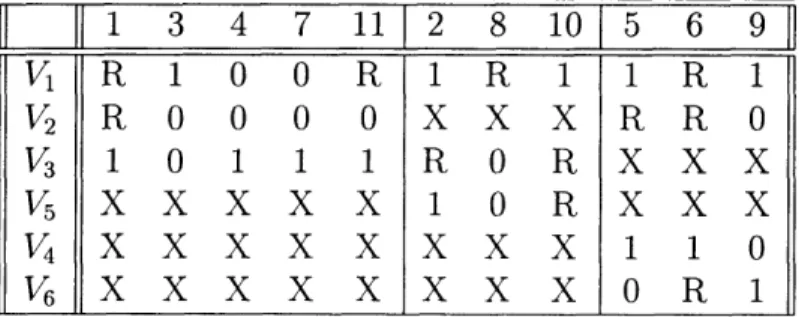
Table 4.1 shows the result of running the partitioning algorithm on the sample set of vectors introduced in Figure 4-1. The vectors have been rearrange to emphasize the reductions in data volume. All the X's in the table specify the scan cells that can be bypassed using Dynamic Scan and represent the direct savings in test data volume and test application time. Other X's have been filled with random values and are represented in the table by "R"s.
4.3.1
Complexity Analysis of the Algorithm
The space complexity of BASIC-PARTITION is O(nm) - the space required to store all the patterns.
algorithm BASIC-PARTITION
1 begin
2 for j = 1 to n
3 initialize cluster Cj to contain only jth scan element
4 create set Dj
5 end
6 while (number of clusters > k)
7 find two clusters C' and C" with minimal DIST(C', C")
8 merge C' and C" into a single cluster C
9 set D = D' U D" 10 end 11 end o(n) 0(1) o(m) o(n) O(n2m) 0(1) O(m)
Figure 4-2: Pseudocode for the BASIC-PARTITION algorithm.
The time complexity requires more attention. Although the creation of the sets
Dj on line 4 takes O(m) steps because each vector needs to be traversed to check
whether it uses a particular scan element, it can be implemented very efficiently with the bit vectors and bitwise operations.
The number of iterations of the while loop in lines 6-10 is O(n - k). However, since typically k <K n, asymptotically there are O(n) iterations.
The most, time consuming operation is finding two clusters with the smallest DIST value. The simplest implementation will calculate the DIST value for every pair of clusters and linearly search for the one with the minimal value. Such implementation will take O(n2m) time while keeping the space requirement linear with number of
Table 4.1: Result of running BASIC-PARTITION
Figure 4-1. "R" represent a randomly filled value.
algorithm on the test vectors of
i 1 3 4 7 11 2 8 10 5 6 9 v1 R 1 00 R I R 1 R i V2 R 000 O O XXXRRO V3 1 0 1 1 1 R O R X XX V5 X X X X X 10 R X X X V4 X X X X X X X 10 V6 X X X X X X X R
scan elements. There are some improvements in this operations at the expense of space, which we will discuss in the next section.
Merging two clusters can be done by changing the pointers of membership in 0(1) time. However, updating the set D is linear with the size of the set (in case when the sets are implemented using bit vectors, the update can be efficiently implemented with the bitwise OR operator).
So the overall runtime of the basic algorithm is O(nm + n n2m) = O(n3
m).
The following section describes how to reduce this runtime at the expense of using additional memory.
4.3.2
Improving the Runtime
There are several improvements that can be implemented to the runtime of
BASIC-PARTITION algorithm. Unfortunately, they all come at the expense of using a multi-plicative factor of O(n) of memory.
The most obvious improvement to the runtime of the algorithm is to avoid calcu-lating the DIST value every time the algorithm searches for a pair with the smallest one. It can be achieved by creating a DIST field for each pair of scan elements and initializing it at the beginning of the algorithm. Later, whenever a pair of clusters is merged together the field can be updated for the relevant pair. If the DIST field values are stored in some ordered way, the search time can also be decreased.
An example of such a data structure that could order the DIST field values is a Fibonacci heap. An element of the heap is a pair of scan elements/clusters with
DIST value being the ordering criterion. Since the pair with the smallest DIST
value is always on the top of the heap the runtime of searching for the pair with the smallest DIST value is 0(1). However, additional work needs to be done to keep the heap consistent.
In our algorithm, whenever two clusters are merged together, the newly created cluster is treated as a single unity and the original two clusters cease to exist. There-fore, all the elements of the heap with reference to the original two clusters have to be removed from the heap and new ones (related to the new cluster) be created
and added to the heap. In order to achieve that, whenever a pair of clusters is merged, O(ra) elements of the heap need to be removed from the heap. In addi-tion, new DIST values need to be calculated for O(n) elements. Each removal of an element for Fibonacci heaps takes O(logn) time; each insertion takes 0(1) time. Therefore, each cluster-merging operation of the algorithm will take O(n(m + log n)) (the factor of m is the time it takes to calculate the new DIST values). Given that
O(n - k) = (n) clusters will need to be merged, the main loop of the algorithm will
take O(n2(m + log n)) time.
The initialization loop will take slightly longer compared to BASIC-PARTITION.
O(n2) heap elements must be created with DIST value calculated for each one and
then inserted into the heap. The INSERT routine for Fibonacci heap takes O(1) time while calculating DIST value takes O(m) time. The total time for initialization is, therefore, 0(n2m).
Thus, the total runtime of the algorithm using Fibonacci heap is O(n2(m +
log n) + n2m) = O(n2(m + log n)). The pseudocode for this algorithm is presented in
Figure 4-3.
4.4
Discussion
There are plenty of other constraints in VLSI design besides optimizing for dynamic scan. Some of these constraints include signal congestion, routing overhead, criti-cal timing path violations. The list can go on [28, 29]. Chapter 3 described how Dynamic Scan architecture leaves plenty of flexibility for the placement tools to re-arrange the scan flip-flops within a segment in a scan chain and even across several chains. However, sometimes some of the placement constraints might have to be violated to maximize the benefits of the dynamic scan and the partitioning algo-rithm returns an unacceptable result from the routing standpoint. The partitioning algorithm described above was designed with flexibility to easily accommodate the additional constraints by simply modifying the DIST metric.
algorithm HEAP-PARTITION
1 begin
2 H - MAKE-HEAP()
3 for i -lto n O(n)
4 initialize cluster Ci to contain only ith scan element O(1)
5 create set Di O(m)
6 for j+-lto i-1 O(n)
7 create the pair { C, Cj} (1)
8 key({Ci, Cj) +- DIST(Ci, Cj) O(m)
9 INSERT(H, {Ci, Cj}) E(1)
10 end
11 end
12 while (number of clusters > k) O(n)
13 {C', C"} +- EXTRACT-MIN(H) O(log n)
14 merge C' and C" into a single cluster C 0(1)
15 D -D' UD" O(m)
16 for each Cj among existing clusters O(n)
17 if (Cj f C' and Cj Z C") then
18 DELETE(H, {C', Cj}) O(log n)
19 DELETE(H, {C", Cj}) 0 (log n)
20 create the pair {C, Cj} o(1)
21 key({C, Cj}) +- DIST(C, Cj) O(m)
22 INSERT(H, {C, Cj)) 0(1)
23 end
24 end 25 end
scan flip-flops are good candidates to be in the same segment. However, they are located far away from each other and placing them in the same segment will be extremely difficult or maybe even impossible1 from the routing point of view. Then no matter how many benefits Dynamic Scan could reap from such a configuration, if the design is inoperable with the two flip-flops in the same segment, the two scan elements cannot be placed together.
With slight modification to the DIST metric, our algorithm can incorporate the additional constraint and return an acceptable result from the first attempt. Let the new metric bl)e
DIST'(Ci, Cj) DISTorig(Ci, Cj) + f(Ci, Cj),
where DISTori9(Ci,Cj) is the original DIST metric defined in Equation 4.3 and
f(Ci, Cj) is some function representing the severity of violating the additional
con-straint if two clusters Ci and Cj are merged together. In the above example, function
f could be the distance between the two clusters. Thus, with the properly adjusted
parameters, the algorithm should find an appropriate solution which takes additional constraints into account.
Chapter 5
The Results
This chapter presents the quality of the partitioning algorithm described in the pre-vious chapter. The results are based on the experimental runs of a HEAP-PARTITION
algorithm implementation. The testcases for our experiments were seven of the largerl ISCAS '89 benchmark designs [12], as well as several designs currently used in indus-try. The specifications of each design are given in Appendix A.
5.1
Experimental Setup
The Dynamic Scan architecture benefits from the presence of X's in the test vectors by means of by-passing them. Therefore, no data volume or test application time can be reduced on the fully specified test vectors. Thus on one hand, having fully specified test vectors reduces the benefits of the Dynamic Scan. On the other hand, not filling X's in the test vectors with random values means giving up the benefit of randomly detecting more faults with fewer vectors. The increase in test vectors translates into additional test data volume, which is contrary to the goal of Dynamic Scan to reduce the test data volume.
Our experiments have shown that if no random fill is used at all, the large increase in the test vector count overshadows the benefits of Dynamic Scan. Our experiments
1Dynamic Scan cannot be used effectively on very small designs because ATPG manages to
achieve 100% test coverage with very few test vectors. Already small quantity of the test data volume does not leave much room for further reduction using Dynamic Scan.
![Figure 1-1: Trend of the cost of manufacturing and testing ASIC designs on per transistor basis [28].](https://thumb-eu.123doks.com/thumbv2/123doknet/14754552.581867/16.933.204.732.119.437/figure-trend-manufacturing-testing-asic-designs-transistor-basis.webp)