HAL Id: hal-00301607
https://hal.archives-ouvertes.fr/hal-00301607
Submitted on 28 May 2004
HAL is a multi-disciplinary open access
archive for the deposit and dissemination of
sci-entific research documents, whether they are
pub-lished or not. The documents may come from
teaching and research institutions in France or
abroad, or from public or private research centers.
L’archive ouverte pluridisciplinaire HAL, est
destinée au dépôt et à la diffusion de documents
scientifiques de niveau recherche, publiés ou non,
émanant des établissements d’enseignement et de
recherche français ou étrangers, des laboratoires
publics ou privés.
L. Melelli, A. Taramelli
To cite this version:
L. Melelli, A. Taramelli. An example of debris-flows hazard modeling using GIS. Natural Hazards and
Earth System Science, Copernicus Publications on behalf of the European Geosciences Union, 2004,
4 (3), pp.347-358. �hal-00301607�
© European Geosciences Union 2004
and Earth
System Sciences
An example of debris-flows hazard modeling using GIS
L. Melelli1and A. Taramelli21Dipartimento di Scienze della Terra, Universit`a degli Studi di Perugia, via Faina, 4, 06123-Perugia, Italy 2Lamont Doherty Earth Observatory of Columbia University, New York, Route 9W, Palisades, NY 10964, USA
Received: 27 March 2003 – Revised: 15 March 2004 – Accepted: 13 April 2004 – Published: 28 May 2004
Abstract. We present a GIS-based model for predicting debris-flows occurrence. The availability of two different digital datasets and the use of a Digital Elevation Model (at a given scale) have greatly enhanced our ability to quantify and to analyse the topography in relation to debris-flows. In particular, analysing the relationship between debris-flows and the various causative factors provides new understand-ing of the mechanisms. We studied the contact zone between the calcareous basement and the fluvial-lacustrine infill ad-jacent northern area of the Terni basin (Umbria, Italy), and identified eleven basins and corresponding alluvial fans. We suggest that accumulations of colluvium in topographic hol-lows, whatever the sources might be, should be considered potential debris-flow source areas. In order to develop a sus-ceptibility map for the entire area, an index was calculated from the number of initiation locations in each causative fac-tor unit divided by the areal extent of that unit within the study area. This index identifies those units that produce the most debris-flows in each Representative Elementary Area (REA). Finally, the results are presented with the advantages and the disadvantages of the approach, and the need for fur-ther research.
1 Introduction
Debris-flows are important geomorphic events in a wide va-riety of global landscapes (Hollingsworth and Kovaks, 1981; Dietrich et al., 1986; Guzzetti and Cardinali, 1992b). There is a sizeable body of literature pertaining to the physical properties of debris-flows (such as Iverson, 1986), where they tend to deposit and the meteorological conditions nec-essary to initiate them (Armanini and Michiue, 1997). In many environments, initiation of debris-flows is in fine-scale valleys in steep, rhythmically dissected terrain. In these ar-eas, concave planform contours define topographic swales,
Correspondence to: A. Taramelli
referred to as “hollows” in the literature (Hack and Goodlet, 1960). Although repeated debris-flows supply much sedi-ment to stream channels and expose bedrock in mountain belts, a significant percentage of debris remains and is stored as a thin colluvial cover, particularly in hollows. These col-luvial pockets act as slope failure “hot spots” by converging infiltration of storm runoff, leading to local groundwater con-centrations above perched water tables and therefore enhanc-ing failure potential. Detritus-filled hollows constitute map-pable debris-flow source areas, which can be identified rou-tinely as potential hazard zones in many intramontane basins and valleys situated in central Italy. Previous studies have mapped many active debris-flows in Umbria (Guzzetti and Cardinali, 1992a). In Umbria, in 2003 Taramelli et al., lo-cated some basins (Menotre area) and related alluvial fans with morphometric and geologic characteristics that would suggest a high disposition to debris-flows but without evi-dence of active debris-flow episodes. In these areas the fans seem to evolve by water flow processes more than debris-flow ones. We suggest that debris-debris-flows in these areas are likely. Thus, there is a need to improve of existing prediction methods and to develop new approaches to identify the trig-gers and the areas of initiation, propagation and deposition of debris flows, including the source areas and the associated upslope water contributing areas. In addition, debris-flow predisposing factors could be identified from a description of the debris-flow prone catchments if attention was given to ge-omorphological and geological landforms, unstable slopes, and superficial deposits.
Use of a GIS model with a statistical and spatial analysis approach ensures an interactive relationship between debris-flows and their causal factors. In this paper, we started from an inventory of hillslope hollows from air photographs and fieldwork in order to map debris-flow events down-slope from initiation sites. Then an analysis of the morphogenetic factors influencing slope instability processes was used to de-fine a Representative Elementary Area (REA). To examine causal relations between the factors and debris-flows events, we calculated an index of debris-flow susceptibility for each
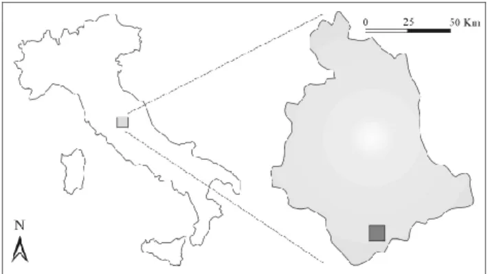
Fig. 1. Location map.
factor in each REA. This was done by dividing the number of debris-flow initiation locations within a particular unit by the areal extent of that unit in the study area. Bivariate statistical methods represent a satisfactory combination between direct mapping methods, based on the subjectivity of the researcher, and data processing using the objective and analytical capac-ities of the GIS.
2 Description of the study area
2.1 Geologic and geomorphologic settings
The study area is located in central Italy (Umbria) along the northern edge of the Terni basin (Fig. 1), a pre-Apennine intramontane basin of the Umbro-Sabino area. In the cen-tral Apennines, the bedrock is a calcareous and marl lime-stone sequence 2200 m thick. The bedrock outcropping in the study area is characterized by a thinly bedded limestone sequence with more marl fraction in the upper part of the se-quence (Calamita and Deiana, 1986). The sese-quence from the bottom to the top is: Calcare Massiccio Fm. (Lower Lias) medium thickness of 800 m and a hemi-pelagic lito-type (Medium Lias – Lower/Medium Miocene). The hemi-pelagic sequence is: Corniola Fm. (300 m thick); Rosso Ammonitico Fm. (50 m), Calcari Diasprigni Fm. (100 m), Maiolica Fm. (300 m), Marne a Fucoidi Fm. (80 m), Scaglia Bianca e Rosata Formation (350 m), Scaglia Cinerea For-mation (150 m), Bisciaro Fm. (70 m), Schlier Fm. (200 m). The Marnoso-Arenacea Fm. (Tortoniano – Messiniano) closes the sequence. The sequence is structured in thrusts and east-verging anticlines and synclines nucleated during a compressive tectonic phase from Oligocene–Miocene to Pliocene (Bally et al., 1986). A subsequent extensional tec-tonic phase controlled all the central Apennines area from the Late Pliocene to present with a maximum value in Lower– Middle Pleistocene (Calamita and Deiana, 1986). Together with this extensional condition isostatic uplift occurred in Lower Pliocene (Ambrosetti et al., 1982). Two sets of normal faults with an Apennines (NW–SE direction) and anti-Apennine (NE–SW direction) trend occurred along the Apennine ridges, producing to intramontane grabens and
semi-grabens such as the Terni basin (Sestini, 1970; Boc-caletti and Guazzone, 1974; Elter et al., 1975). The Terni basin is a semi-graben, with a rectangular shape, 15 km long (E–W direction) and 8 km wide (N–S direction). The old-est sediments that outcrop there are datable from Lower Pleistocene–Late Pleistocene (Basilici, 1993). The northern edge of the basin is bounded by the southward edge of tani ridge along an important regional discontinuity: the tana Fault. The Umbrian sequence outcrops along the tani Mounts is abruptly interrupted southward along the Mar-tana Fault with an eroded and continuous edge scarp. This is a massive (between 700 m and 900 m), steep and wooded slope, in calcareous bedrock, with incisions made by streams, which cut the fault scarp into triangular facets (Fig. 2). The fault north of Cesi (Fig. 2) trends N160 with normal dis-placement toward the south, turning just east of Cesi to-wards N120. From Cesi to Rocca San Zenone, the scarp decreases in width. Faulting led to the uplift, erosion and re- sedimentation of the sedimentary infill in the formerly active basin (Cattuto et al., 2002). A large apron outcrops along the contact between the limestone ridge and the Terni basin over fluvial–lacustrine (Plio-Pleistocene) and alluvium deposits. Within the basin there are continental deposits dat-able from the Plio-Pleistocene. The sequence is made up of four lithostratigraphic formal units (Basilici, 1993): lower grey clay unit (upper Pliocene); clayey sandy silt unit (lower Pleistocene); upper sandy gravel unit (lower- middle Pleis-tocene); Old Travertine unit (unconformable previous). Ly-ing on these sediments are talus, fans and travertine, recent in age. Along the alluvial fan area, further south, two ad-ditional faults parallel to the Martani Mountains fault are recognisable with ESE–WNW trend (Cattuto et al., 2002). Toward the north the slope’s appearance changes beyond the village of Cesi. The mountain is bounded by a narrow bench cut by streams that wash the scarp before entering the San Francesco gully, which runs parallel to the steep slope, dom-inated on its right bank by the hill of San Gemini (280– 350 m).
2.2 Climatic setting
Climate in Umbria is Mediterranean, with wet winters and dry summers. Average annual rainfall ranges from 1000 to 1200 mm/year. The highest rainfall values occur in Novem-ber, and minima are in July and in March (Table 1). The main triggering factor for debris-flows occurrence is pro-longed rainfall. Table 2 shows heavy expected rainfall values predicted for the Terni area (Regione dell’Umbria Servizio Idrografico, 1990). An historical record of the relation be-tween rainfall and debris-flows is not available for the study area. However the highest expected rainfall values in the area are enough to trigger debris-flows. This is based on a com-parison with investigations in other Italian area (Bacchini and Zannoni, 2003). Furthermore, the climatic trend in the area, and in central Italy, is toward an increase in the number of heavy rainfall days (Dragoni, 1998). A decreasing trend for moderate rainfall and an increasing trend for temperature are
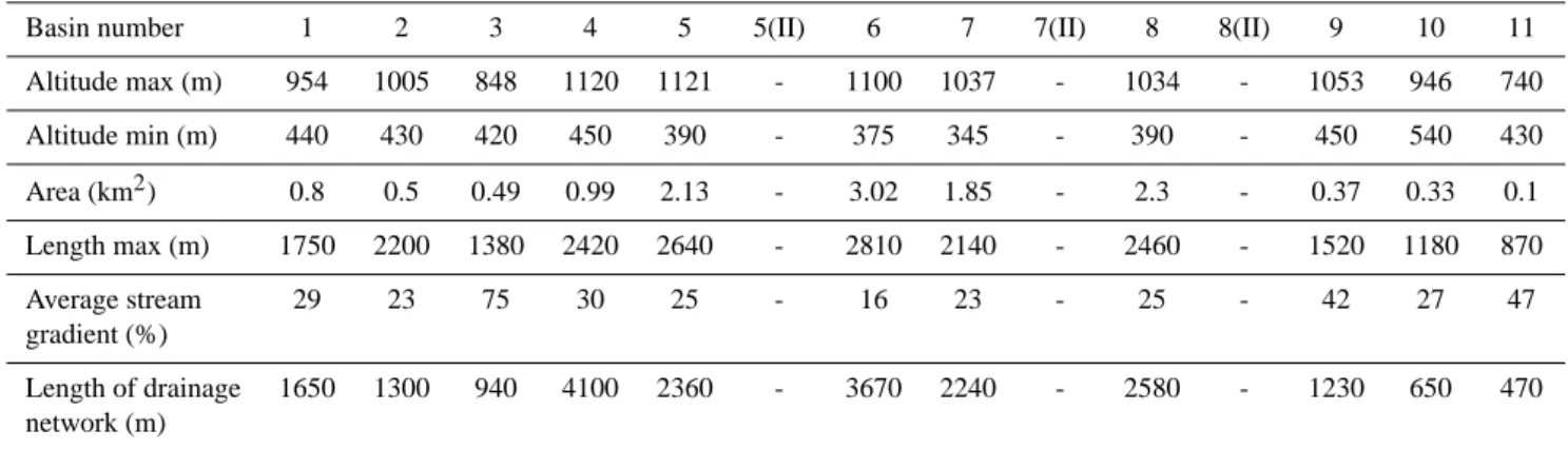
Fig. 2. Geological map: 1) Alluvial deposits; 2) Fluvio – lacustrine deposits; 3) Talus deposits; 4) Colluvial deposits; 5) Fan (first generation);
6) Fan (second generation); 7) Scaglia rossa Formation; 8) Fucoidi Formation; 9) Maiolica Formation; 10) Diasprigni – Rosso ammonitico – Corniola Formations; 11) Calcare massiccio Formation; 12) Martana Faults; 13) Normal Fault; 14) Martani Mountains Bedrock. The letters are referred to basins name. In order: 15) San Francesco, 16) Cantaretto, 17) Santa Maria di Fuori, 18) Sant’Andrea, 19) Schiglie, 20) Val di Licino, 21) Val di Noce, 22) Calcinare, 23) Torricella-Cisterna, 24) Torricella-Villa Francia, 25) Torricella-Villa de Angelis.
Table 1. Rainfall statistics from the 4 gauging stations within 14 km of the study area.
Locality Lat. Long. Altitude Years* Rainfall Days of rain Basin m s.l.m. (mm/year)
Stroncone 42◦30’ 00” 12◦12’ 16” 451 51 1015 77 Nera Terni 42◦33’ 40” 12◦38’ 53” 170 22 1006 - Nera Sangemini 42◦36’ 50” 12◦05’ 32” 170 52 1115 80 Nera Marmore 42◦37’ 50” 12◦15’ 37” 377 20 1161 20 Velino * Numbers of years considered for the evaluation of the mean annual precipitation.
expected, which are in agreement with an increase in the number of heavy rainfall days (Trenberth, 1999). Whyte (1995) shows that an increase in heavy rainfall events is re-lated to a reactivation of shallow landslides (as debris-flows) with a larger mobilization of talus along the slopes.
3 Data sources and database
3.1 Morphometric characteristics of the basins
Eleven catchments and the corresponding alluvial fans were identified and digitized within a Geographical Information System (GIS) using 1:10 000 scale topographic maps and in-terpreted 1:13 000 black and white aerial photographs taken
in 1998. Morphometric characteristics were then obtained from small scale topographic maps and by using a algorithm that imposed single pixel outflow from a regional-wide DEM with a ground resolution of 25 m (Guzzetti and Reichenbach, 1994). Due to the resolution of the DEM, the catchment area (15.3 km2) was estimated by dividing the area of each pixel by the average of the computed catchment slopes. An at-tempt was made to describe river catchments based on mean of elevation, stream gradient and catchments areas (Table 3).
The eleven catchments are:
1) San Francesco, 2) Cantaretto, 3) Santa Maria di Fuori, 4) San Andrea, 5) Schiglie, 6) Val di Licino, 7) Val di Noce, 8) Calcinare, 9) Monte Torricella – Cisterna, 10) Monte Torricella – Villa Francia, and 11) Monte Torricella – Villa de Angelis.
Table 2. Expected maximum rainfall values (mm) for Terni rain
gauge station (Lat. 42◦ 33’ 40”; Long. 12◦ 38’ 53”; Alt. 130 m a.s.l.).
Expected rainfall (mm) 1 3 6 12 24 (hours) Values for 5 years 41 62 80 95 113 Values for 10 years 49 73 90 107 128 Values for 25 years 59 87 103 121 147 Values for 50 years 66 97 112 133 161 Values for 100 years 74 107 122 144 175 Values for 500 years 91 131 144 168 208
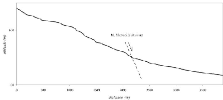
The catchments have different morphologies due to differ-ent clay percdiffer-entage. All the catchmdiffer-ents are on calcareous bedrock with different clay-marly/limestone ratio. The mul-tilayer is a sequence of formations with a high percentage in limestone in the lower part and a significant percentage of clay in the upper one. Basins in the centre of the study area (e.g., n. 6 Val di Licino and n. 7, val di Noce), have a high percentage of clay. All the catchments have a limited devel-opment longitudinal profile due to presence of the Martana fault, restricting the average area of the eastern basins to a few tens of square kilometres. Total relief ranges between 390 m and 790 m, with a lower mean elevation. Because of the presence of the Martana fault, the streams reach only the second order and are in a non-equilibrium condition. The stream longitudinal profiles are not graded profiles; there is a clear convexity in the upper part and frequent drops along all the basament portion of the profile (Fig. 3). The mean catch-ment area is 1.1 km2the maximum is 3.02 km2(Val di Licino basin) and the minimum is around 0.10 km2(M. Torricella – V. la de Angelis basin). Larger catchment areas are found between the Schiglie basin and the Calcinare basin, which have the highest mean elevation and mean slope. The mean stream gradient is about 33%; lower values are found for the fans located in the central part of the scarp fault.
3.2 Fan morphometry
The identification and mapping of fans was carried out in the field, by using topographic maps and interpreting two sets of black and white aerial photographs (scale 1:13 000 scale, flown in 1978 and 1988). The boundaries of the fans were also crosschecked using a digital derivate hillshade from the 25 m DEM. The fan boundaries were drawn interactively on the shaded relief map based on the spatial distributions of slope, local relief and curvature. The steepest terrain was found at the apexes of the fans or along the scarp gener-ated by the faults activity (Fig. 2; Cattuto et al., 2002). As a consequence of the presence of the two faults a major west-ward opening has generated two main bodies in the fans of
Fig. 3. Longitudinal profile of Val di Noce river shows frequent
drops along the profile on the basement portion. The fault draws the transition between the bedrock basament (upstream) and the fan deposits (downstream).
the Schiglie basin, Val di Licino basin and Calcinare basin. In these areas it is possible to divide fans into three thik-ness units (borehole data acquired by Martinelli and San-tucci, 1995): from the M. Martani fault to 200 m a.s.l. the maximum thikness is around 50 m. The second zone has a thickness between 30 m and 50 m from 200 m a.s.l. to 170 m. The third zone is characterised by a thikness below 30 m. All the alluvial fans show fanhead trenching. For each of the investigated fans we computed a set of morphometric char-acteristics from the 25 m DEM (Table 3). The fans have an average area around 0.8 km2, an average slope gradient of 12.5%, an average length of 1.3 km and of width 0.9 km. 3.3 Hollow identification
The presence of hollows and hydrologic conditions are the critical combination that causes debris-flow events (Reneau and Dietrich, 1987; Deganutti and Marchi, 2000). The long recurrence intervals and the apparent importance of high in-tensity rainfall events indicate that a lack of historic debris-flows from specific hollows is by no means an indicator of future stability. Furthermore, quantitative debris-flow as-sessment is complicated by the observation that debris-flows typically involve these hollows and that several debris-flows can be released from a single hollow over many years. It is important to predict which hollows are most vulnerable to failure, how much of the colluvium will fail, and where the resulting debris-flow will come to rest. To do this we must know where volumes of debris are located on hill-slopes within hollows and define mappable debris-flow haz-ard source areas.
Identification of the hollows from aerial photographs may be difficult where colluvial deposits in subtle topographic de-pressions are hidden by forest. Classifying colluvium- filled hollows depends upon identifying the extent of colluvial fill. Geomorphic mapping provides a practical approach, as the margins of colluvial deposits in hollows are generally coin-cident with a change from convex to concave slope profile. Thus areas of convex planform contours often approximately correspond with the dimensions of a colluvial deposit: hol-lows are likely to exist where contours are concave-out from
Table 3. Morphometric characteristics of basins and fans identified by number shown in Fig. 2. The numbers marked by (II) represent basins
with fans prograding in two main lobes.
Basin number 1 2 3 4 5 5(II) 6 7 7(II) 8 8(II) 9 10 11
Altitude max (m) 954 1005 848 1120 1121 - 1100 1037 - 1034 - 1053 946 740 Altitude min (m) 440 430 420 450 390 - 375 345 - 390 - 450 540 430 Area (km2) 0.8 0.5 0.49 0.99 2.13 - 3.02 1.85 - 2.3 - 0.37 0.33 0.1 Length max (m) 1750 2200 1380 2420 2640 - 2810 2140 - 2460 - 1520 1180 870 Average stream 29 23 75 30 25 - 16 23 - 25 - 42 27 47 gradient (%) Length of drainage 1650 1300 940 4100 2360 - 3670 2240 - 2580 - 1230 650 470 network (m)
Fan number 1 2 3 4 5 5(II) 6 7 7(II) 8 8(II) 9 10 11
Altitude max (m) 440 30 420 450 390 275 375 345 248 390 235 450 540 43 Altitude min (m) 298 273 225 224 190 140 160 225 198 174 190 200 235 250 Width max (m) 520 1130 520 1100 1550 860 1870 770 350 1370 400 850 950 470 Length max (m) 900 1140 1000 1380 1640 1680 2070 1050 870 1830 710 1750 1530 860 Average slope 14 14 14 16 12 8 10 11 7 8 7 14 21 19 gradient (%) Area (km2) 0.3 0.72 0.32 1.42 1.37 1.1 2.5 0.26 0.13 1.98 0.15 0.77 0.4 0.26
the slope, contrasting with side slope and ridges where con-tours are straight and convex respectively.
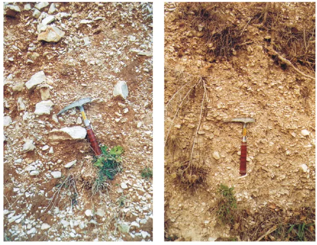
Source areas of debris-flows (hollows) can be classified in four main environments in central Apennines: landslide de-posits, highly fractured rocks in sheared zones of regional normal faults, talus slopes and glacial deposits (Guzzetti and Cardinali, 1992b). In the Terni area we have identified only two types in the eleven basins. The volume and type of de-bris depend on lithology, weathering activity, slope surface, vegetation covers, land use and river erosion capacity. The first type (1st hollow, type-r), immediately releasable, is lo-cated at the base of the slope. It is poorly consolidated and is generated either from mass movements or talus deposits. The second type (2nd hollow, type-n), eluvial-colluvial de-posits, is accumulated by the weathering, and are most abun-dant where the channel initiates. The border of these basins present low slope relief. Thus the top of the drainage system is characterized by low debris flow acclivity with greater ac-cumulation. In addition, rates of accumulation of colluvium could vary greatly between sites, and deposit size should thus be reached at different times in different hollows. Deposits with non- matrix supported colluvium are generally scattered through time, with the timing of failure controlled in part by the depositional rate of colluvium and the strength provided by vegetation and by high intensity rain. In this case, the
estimated depth of in-channel deposits and the extent of the potential debris supply areas (1st hollow, type-r), have a vari-able mean thickness. On the contrary to these typically steep sites, a large amount of colluvium (old in-channel deposits partly stabilized – 2nd hollow, type-n), is stored in rela-tively stable deposits with a mean thickness of 1.5–2 m. This kind of hollow includes sites with low slope gradients and sites where hydrologic conditions allow subsurface drainage (Fig. 4).
To mobilize these colluvial deposits it is necessary to have particular and non frequent conditions such as unusually high-intensity rainfalls that result in elevated pore pressures. Quantitative analysis of the landform in the study area iden-tifies many catchments where it is possible to apply a pre-dictive equation for assessing the magnitude in terms of vol-ume of a debris flow. The equation has been tested in dif-ferent catchments in the Alps (Tropeano and Turconi 1999). The equation estimates the magnitudo or total displaced vol-ume estimated in each basin for paroxystic rainfall events,
V, based on the effective catchement area, 1E, in km2, the average catchment slope, tgs, the areal extent of materials likely to move, r, the mean estimeed depth of the debris, h, the percentage of debris available in a large time range, n, and a frequency factor, f .
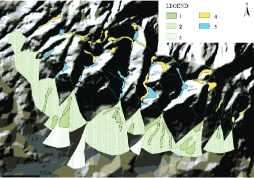
Fig. 4. Geomorphological map: 1) Debris-flow deposits; 2) Fan (first generation); 3) Fan (second generation); 4) Hollow Deposits n type;
5) Hollow Deposits r type.
Table 4. Catchments statistics where V = total displaced volume estimated, 1E= effective catchment area (km2), tgs= average catchment slope, the r= areal extent of materials likely to move / 1E, h= estimated mean depth, n= % of debris available in a larger time range,
f =frequency factor. Rivers 1E tgs r h n f V (km3) 1) San Francesco 0.8 29 0.17 3 - 1 0.032 2) Cantaretto 0.5 23 0.08 3 0.06 1 0.008 3) S. M. di Fuori 0.49 75 0.1 3 - 1 0.03 4) Sant’Andrea 0.99 30 0.09 3 0.06 1 0.02 5) Schiglie 2.13 25 0.13 3 0.03 1 0.06 6) Valle di Licino 3.02 16 0.07 3 0.04 1 0.03 7) Val di Noce 1.85 23 0.13 3 0.16 1 0.05 8) Calcinare 2.3 25 0.05 3 0.03 1 0.02 9) Torricella-Cisterna 0.37 42 0.22 3 - 1 0.003 10) Torricella-V. la Francia 0.33 27 0.09 3 - 1 0.007 11) F. na della Mandola 0.1 47 0.6 3 - 1 0.02
The equation is given as:
V = [1E × tgs × r × h × (n +1) × ef]/1000 . (1) Table 4 shows the estimated total volume of debris avail-able for debris flows in each basin.
Different relationships between catchments and factors causing debris-flows can be pointed out. The mean value of the total displaced volume is estimated to be 0.03 km3.
Going east to west, tectonic influence on basin development is due to the major opening of the fault system. Sites with large drainage areas, that typically include the two different types of hollows, are more influenced by the disequilibrium conditions in the catchment areas. Consequently, the central basins have high values of total removable volume.
In the fans, interpretations of aerial photographs showed many deposition episodes on the fans’ surface that are not
Fig. 5. Debris-flows deposits near the intersection point of Val di Licino fan.
easily observed in the field. Differences in texture and tonal-ity are still evident in extended deposits, in spite of the inten-sive agricultural land use. These tongue deposits are prob-ably different depositional episodes linked to debris-flow events. Debris-flow deposits appear most often on the upper fan (Fig. 5), while alluvial deposits are more frequent below of the intersection point, which is the point where the major channel of deposition intersects the surface.
4 GIS analysis
4.1 Correlation between debris-flows and their causal fac-tors
The first step in our analysis consists in defining precisely the meaning of debris-flow hazard. Debris-flow hazard indi-cates the probability that a given event will take place within a given time period (Varnes, 1984). Although debris-flows are often caused by single triggering events, such as heavy rains or human activity, they depend on several primary fac-tors that make slopes susceptible to failure, such as geometry, lithological- structural and hydrographic characteristics (Lin et al., 2002). Based on the tables compiled and on field ev-idence a total of four factors (geology, slope, distance from rivers and distance from faults) were selected. For the geo-logic factor the original multilayer sequence was grouped in
five classes according to the lithology (percentage of lime-stone and clays) and the bedding thickness. The Corniola, Calcare Diasprigni and Rosso ammonitico formations were grouped in a single class because of their lithology. Once the identification and mapping of the factors was done, the maps were digitized. This operation involved the conver-sion from vector format into raster format for analysis in a GIS environment. The difficulty with this conversion lies in the choice of the type of Representative Elementary Area (REA). Because it influences the structure and the character-istic of the database and the reliability and the precision of the analysis (Westen van et al., 2000). If very small pixel sizes are chosen, the statistical relation will be large, but the matrices for managing mathematical operations will be too voluminous. On the other hand, the use of larger pixels in-duces errors in assessing the actual presence or absence of hollows when it involves only a small part of the reference units, and consequently it induces errors in the assessment of the relationships between intrinsic factors and debris-flows. Moreover REAs are treated as homogenous spatial domains in relation to the intrinsic factors and the degree of hazard. After a few trials, we determined that cells of 25×25 m pro-vided sufficient detail, while requiring fairly short processing times. We used 24 411 pixels for a study area of 15.3 km2. The second step in our analysis consisted in estimating the contribution of each causative parameter is the analysis, in a
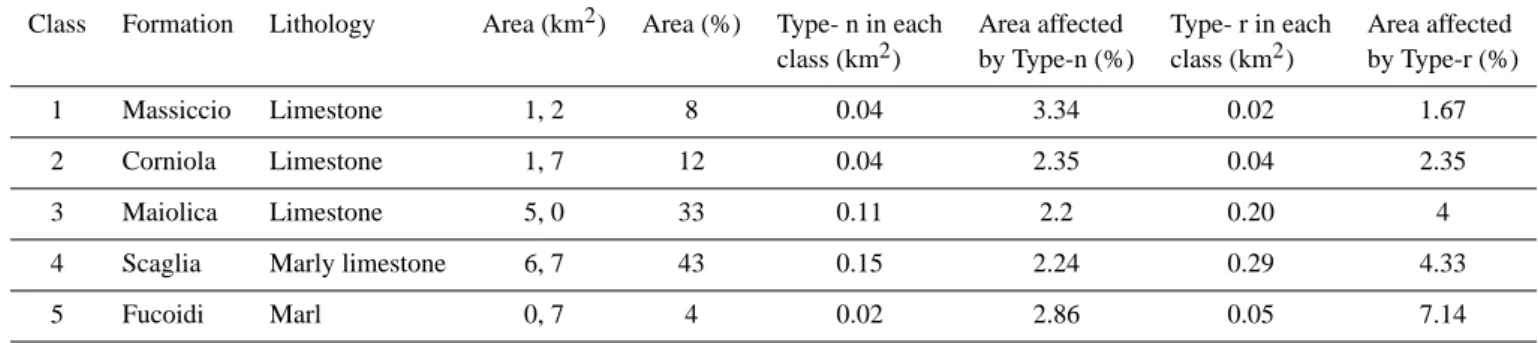
Table 5. The spatial distribution of hollows densities for the two factors maps (geology and slope).
Class Formation Lithology Area (km2) Area (%) Type- n in each Area affected Type- r in each Area affected class (km2) by Type-n (%) class (km2) by Type-r (%)
1 Massiccio Limestone 1, 2 8 0.04 3.34 0.02 1.67
2 Corniola Limestone 1, 7 12 0.04 2.35 0.04 2.35
3 Maiolica Limestone 5, 0 33 0.11 2.2 0.20 4
4 Scaglia Marly limestone 6, 7 43 0.15 2.24 0.29 4.33
5 Fucoidi Marl 0, 7 4 0.02 2.86 0.05 7.14
Class Slope (%) Area (km2) Area (%) Type- n in each Area affected Type- r in each Area affected class (km2) by Type-n (%) class (km2) by Type-r (%)
1 0◦–13◦ 2.1 13.8 0.06 2.86 0.22 10.48
2 13◦–26◦ 6.9 45.1 0.14 2.03 0.37 5.37
3 26◦–40◦ 5.9 38.6 0.15 2.54 0.01 0.17
4 40◦–53◦ 0.3 1.9 0.01 3.33 -
-5 53◦–66◦ 0.1 0.6 - - -
-Class Area (km2) Type-n (km2) Area affected by Type-r (km2) Area affected by Type-n (%) Type-r (%)
River 2.8 0.4 5.36 0.6 13.57
Discontinuity 2.9 0.4 3.25 0.6 13.1
GIS environment, of the digitized data, to estimate the con-tribution of each causative parameter toward instability. This contribution can be expressed by means of a quantitative pa-rameter such as the linear regression coefficient R2(Barredo et al., 2000; Taramelli et al., 2003). The geological map and the slope map used in the analysis were normalized with re-spect to the hollows map. This was done to ascertain the presence/absence of hollows in all classes of each individual factor, and to obtain the value of the R2 correlation coeffi-cient (Naranjo et al., 1994; van Westen, 2000). The method-ology involved three steps. In the first step we extracted from the geologic map five GRIDs, each corresponding to a ge-ological class in the map. The slope map was also classi-fied into 5 classes, and a separate GRID was obtained from each class. In the second step, the individual GRIDs were compared with the map of hollows (in GRID format), and the presence or absence of hollows in each pixel was ascer-tained. The result of the calculation was converted into an-other GRID that contains only pixels in which hollows were present. Lastly, in the third step we converted the number of pixels into square kilometers, and we obtained the area af-fected by hollows in each class. The results of our analysis are shown in Table 5. In the Scaglia and Maiolica Formations slopes ranging between 13◦–26◦(class 2, 45.0% of the area)
and between 26◦–40◦(class 3, 38,6% of the area) are most
abundant. Most of type-r and type-n deposits in the hollows are present in these two classes. In particular, we observe that:
1) Hollow deposits type-n are found in all formations with a minimum value of 2.2% in Maiolica Formation and a maximum value of 3.34% in the Massiccio Formation; 2) Deposits of type-n are abundant where the terrain is
steeper (class 4, 40◦–53◦). The deposits are present at the top of the main channel. These parts of the catch-ment areas have low slope relief and low values of elu-vial and colluelu-vial angles of repose. So all the basin threshold area is characterized by high relief except the hollows accumulation zones. Due to the choice of the pixel as the REA the reclassification of slope in DEM analysis induces error because it considers only areas bigger than REA. This caused the lack of these pixels. 3) Deposits of type-r are well represented in Fucoidi
For-mation (7.14%). In contrast the Massiccio ForFor-mation is not significant for this type of hollows because of the tendency toward slope instability in these forma-tions (greatest in Fucoidi with a high percentage of marl
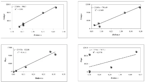
Fig. 6. The empirical relationship linking the lithology factor and the slope gradient factor to the presence of hollows has been found to be a
linear correlation R2.
Fig. 7. Parameter weights were assigned for each factor class, based on the comparison of total density with the individual densities of
hollows (r and n types) in each class.
fraction and lowest in Massiccio, a massive limestone formation).
4) Deposits of type-r are uncorrelated to debris-flows be-cause of the large range of their angle of repose. This is due to different local percentages of clay in the deposits due to the different source materials.
The values for the parameter class/hollow area pairs, normal-ized for the total areas (i.e., total area occupied by the factor and total area of the hollow), were used in the calculation
of R2 in order to link empirically geology and slope to the presence of hollows (Fig. 6).
Based on the presence or absence of hollows in the individ-ual classes, the third step in the analysis consisted in calculat-ing a weight assigned through a statistical validity function. For the purpose, we used the approach described by Naranjo et al. (1994).
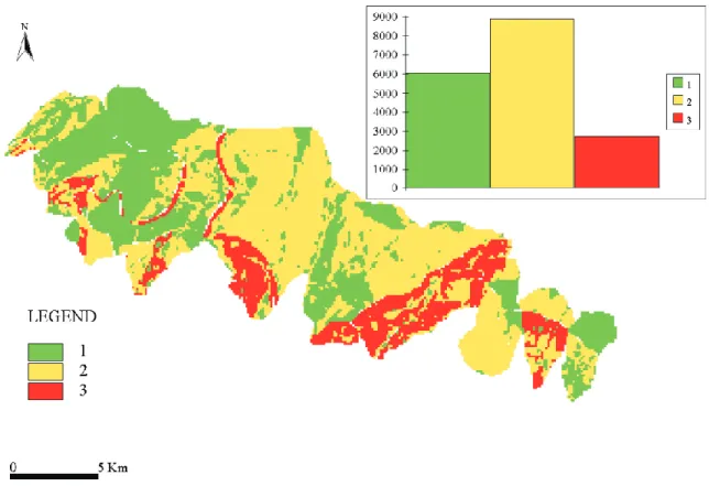
Fig. 8. Map of the study area showing susceptibility to debris-flows: Class I: areas with a low propensity toward debris-flow; Class II: areas
a medium propensity toward debris-flow; Class III: areas with a high propensity toward debris-flow.
Where Wfi is the weight assigned to the i-nth class of the
factor f considered; Af iis the area the type-r hollow in the
i-nth class of the factor f and Aciis the area of the i-nth class;
Af is the total hollow area.
We use Eq. 2 to evaluate the susceptibility to debris-flows for both classes, in comparison with the number of hollows in the entire study area. Geology and slope were reclassified using values ranging between 1 and 5. The value 5 was given to the classes that were considered potentially most unstable. For type-r deposits, the Fucoidi Formation exhibits the high-est weight in debris-flow evaluation. For type-n deposits, the Fucoidi and Massiccio Formations are relevant. Two slope classes are important, namely 0◦–13◦and 40◦–53◦, for both type-n and type-n deposits (Fig. 7). For the parameters de-scribing the distance from the streams and the distance from the faults, we estimated the weight using a heuristic proce-dure, which consisted in overlaying the maps representing these two parameters on the landslide hollow maps in a GIS environment. By map intersection we evaluated the relation-ship between the presence of the factor and that of the hol-lows. Inspection of the results revealed a relation between the presence of these factors and that of the hollows. To dis-criminate the areas most susceptible, a buffer of 50 m was considered around both the faults and the drainage. Weights were assigned decreasing linearly within the mapped area of influence (Table 5).
The last step consisted in the classification of the study area into domains, based on different susceptibility. We prea-pared the debris-flows susceptibility map by multiplying the weights of the classes by the weights of the parameter maps, and by summing the weights for each pixel. The resulting map was further reclassified into 3 susceptibility classes, for improved readability (Fig. 8). The three classes portray:
1) generally stable areas;
2) areas with a low propensity toward debris-flows; 3) areas with a high propensity toward debris-flows.
The first class (13% of the study area) comprises area where limestone, sandyconglomerates, and eluvial deposits crop out. To the second class (37% of the study area) belong the areas characterized by medium terrain gradient (10◦–
20◦), mainly present at the end of the slopes. The third class
(35% of the study area) comprises areas with steep slopes (>20◦), usually deeply carved by streams or affected by in-creased erosion due mainly to tectonic activity also under-lined by the two orders of the fans (Cattuto et al., 2002). Belonging to the third class are also the talus areas, or the areas were debris deposits are present along the slope and the hollow. These debris deposits, having been previously involved in debris-flow phenomena, exhibit poor mechanical characteristics in our opinion.
5 Conclusions
Our results, which are based on hollows inventory from aerial photography, field mapping, and the GIS modeling are the follows:
1) The study area has favorable characteristics for debris-flows occurrence because of the geological setting of limestone bedrock and numerous hollows along the slopes. Hollows development depends either upon the presence of unconsolidated deposits or upon the presence of the old in-channel deposits partly stabi-lized, debris that becomes mobilized and incorporated into the fluid mass during major floods. Deposits in a topographic hollow are considered potential debris-flows source areas. These colluvial pockets act as slope failure “hot spots” by focusing infiltration of storm runoff, leading to local groundwater concentra-tion above perched water tables and therefore enhanced failure potential.
2) We have identified the terrain attributes related to the occurrence of debris-flows and quantified their relative contribution to the susceptibility of debris-flow events. Morphometric characteristics of basins and fans under-lie the relationships among sediment transport, hills-lope hydrologic properties and shills-lope stability that gov-ern the association of debris-flows with hollows. De-bris moves down-slope as a result of mass wasting pro-cesses. Where overland flow is either non-erosive or infrequent, colluvium accumulates along the line of de-scent. Topographic convergence also focuses subsur-face runoff into hollows. Debris accumulations in and along alluvial fans are the depositional areas for debris-flows originating in upslope hollows and channels. 3) The GIS-based method presented is a promising tool
to use to investigate debris-flows in different water-sheds. Using bivariate statistical methods, the combi-nation of different causative parameters (in regard to debris-flows) may constitute the basis for an objective assignment of weight. For each basin the susceptibility index could be calculated as the number of hollow loca-tions in a primary factors unit divided by the areal extent of that unit. Analysis of the debris-flow causative fac-tors allowed determining the sources of the variations in debris-flows response in the drainage basins.
4) The results of the research also show that there are lim-itations to the use of bivariate statistical methods. The methodology needs a careful confrontation with the real world with respect to the practical use of the concept of the REA, leading to the conclusion that an itera-tive process would optimize the methodology. More-over the spatial relationship between causative factors and debris-flow evaluation is improved if other variables are considered such as climatic trends or wildfire occur-rence in the wooded catchment areas.
Acknowledgements. The authors are grateful to the two unknown
referee for their useful review and for suggestions and interest through it all. We would also like to acknowledge the support of C. Stark for much needed advice and to R. A. Weissel especially for her help in the English language.
Edited by: F. Guzzetti Reviewed by: two referees
References
Ambrosetti, P., Carraio, F., Deiana, G. and Dramis, F.: Il sollevamento dell’Italia centrale tra il Pleistocene inferiore e il Pleistocene medio, Contrib. Concl. Realizz. Carta Neotet-tonica d’Italia (parte II), Progetto Finanziato Geodinamica Sottoprogetto-Neotettonica CNR, 513, 219–223, 1982.
Armanini, A. and Michiue, M.: Recent Development on Debris-Flows, Springer, New York, 1997.
Bacchini, M. and Zannoni, A.: Relations between rainfall and trig-gering of debris flow: case study of Cancia (Dolomites, north-eastern Italy), Natural Hazard and Earth System Sciences, 71–79, 2003.
Bally, A. W., Burbi, L., Cooper, C., and Ghelardoni, P.: Balanced sections and seismic reflections profiles across the Central Apen-nines, Memorie Societa’ Geologica. Italiana, 35, 257–310, 1986. Barredo, J. I., Benavides, A., Herv´as, J., and van Westen, C. J.: Comparing heuristic landslide hazard assessment techniques us-ing GIS in the Tirajana basin, Gran Canaria Island, Spain, Inter-national Journal of Applied Earth Observation and Geoinforma-tion, 2, 9–23, 2000.
Basilici, G.: Il Bacino continentale Tiberino (Plio-Pleistocene, Um-bria): analisi sedimentologica e stratigrafica, Tesi di Dottorato, V◦ciclo, Universit`a degli Studi di Bologna, 1993.
Boccaletti, M. and Guazzone, G.: Remnant arcs and marginal basins in the Cenozoic development of the Mediterranean, Na-ture, 252, 18–21, 1974.
Calamita, F. and Deiana, G.: Geodinamica dell’Appennino umbro-marchigiano, Memorie Societa’ Geologica. Italiana, 35, 311– 316, 1986.
Cattuto, C., Gregori, L., Melelli, L., Taramelli, A., and Troiani, C.: Paleogeographic evolution of the Terni basin (Umbria, Italy), Bollettino Societa’ Geologica Italiana, Vol. Spec. 1, 865–872, 2002.
Deganutti, A. M. and Marchi, L.: Rainfall and debris-flow occur-rence in the Moscardo basin (Italian Alps), Prediction and As-sessment, Wieczorek, G. and Naeser, N., A.A. Balkema, Rotter-dam, 67–72, 2000.
Dietrich, W. E., Wilson, C. J., and Reneau, S. L.: Hollows, col-luvium and landslides in soil-mantled landscapes, in: Hillslope processes, edited by Abrahams, A. D., Allen and Unwin, Boston, MA, 361–388, 1986.
Dragoni, W.: Some Considerations on Climatic Changes, Water Re-sources and Water Needs in the Italian Region South of 43◦N, in: Water, Environment and Society in Times of Climatic Change, edited by Issar, A. S. and Brown, N., 241–271, Kluwer Ac. Pub., Printed in Netherlands, 1998.
Elter, P., Giglia, G., Tongiorgi, M., and Trevisan, L.: Tensional and compressional areas in the recent (Tortonian to present) evolu-tion of the Northern Apennines, Bollettino di Geofisica Teorica e Applicata, 17, 3–18, 1975.
Guzzetti, F. and Cardinali, M.: Debris-flow phenomena in Central Apennines of Italy, Terra Nova, 3, 619–127, 1992a
Guzzetti, F. and Cardinali, M.: Debris-flow phenomena in the Umbria–Marche Apennines of central Italy, Int. Symp. Inter-praevent, Bern, Tagungspublikation, Band 2, 181–192, 1992b. Guzzetti, F. and Reichenbach, P.: Towards a definition of
topo-graphic division for Italy, Geomorphology, 11, 57–74, 1994. Hack, J. T. and Goodlett, J. C.: Geomorphology and forest
ecol-ogy of a mountain region in the central Appalachians, U.S. Geol. Survey Prof. Paper 347, USGS, Denver, CO, 1960.
Hollingsworth, R. and Kovaks, G. S.: Soil slump and debris flows: prediction and protection, Bull. of the Ass. of Engine. Geol., XVIII, 1, 17–28, 1981.
Iverson, R. M.: Ground-water seepage vectors and the potential for hillslope failure and debris flow mobilization, Water Resour. Res., 22, 1543–1548, 1986.
Lin, P. S., Lin, J. Y., Hung, J. C., and Yang, M. D.: Assessing debris-flow hazard in a watershed in Taiwan, Engineering Geology, 66, 295–313, 2002.
Martinelli, A. and Santucci, A.: Idrogeologia delle sequenze conti-nentali, in: Studi sulla vulnerabilit`a degli acquiferi, 10, Pitagora Ed. Bologna, 29–56, 1995.
Naranjo, J. L., van Westen, C. J., and Soeters, R.: Evaluating the use of training areas in bivariate statistical landslide hazard anal-ysis – a case study in Colombia: ITC Journal, 1994-3, 292–300, Enschede, 1994.
Regione dell’Umbria Servizio Idrografico: Analisi ed elaborazione delle precipitazioni di massima intensit`a e di breve durata inter-essanti i bacini umbri, Quaderni della Regione dell’Umbria, vol-ume speciale, 1990.
Reneau, S. L. and Dietrich, W. E.: The importance of hollows in de-bris flow studies; examples from Marin Country, California, in: Debris Flows/Avalanches: Process recognition and Mitigations, edited by Costa, J. E., and Wieczorek, G. F., Geol. Soc. of Amer. Rev. of Engin. Geol., vol. 7, 165–180, 1987.
Sestini, G.: Postgeosynclinal deposition, in: Development of the Northern Apennines Geosyncline, edited bu Sestini, G., Sedi-mentary Geology, 4, 481–520, 1970.
Taramelli, A., Melelli, L., Cattuto, C., and Gregori, L.: Debris flow hazard mitigation using GIS: an example in the F. Menotre Basin (central Italy), Int. Conference on: “Fast Slope Movements – Prediction and Prevention for Risk Mitigation” Sorrento, May, 11–13, 485–489, 2003.
Trenberth, K. E.: Conceptual framework for changes of extremes of the hydrological cycle with climate change, Climatic Change 42, Kluwer Academic Publishers, Printed in The Netherlands, 327–339, 1999.
Tropeano, D. and Turconi, L.: Valutazione del potenziale detritico in piccoli bacini delle Alpi occidentali e centrali, Pub. N.2058 – Gruppo Nazionale Difesa Catastrofi/Consiglio Nazionale Ricerche, 1999.
Varnes, D. J. and IAEG Commission on Landslides and other Mass-Movements: Landslide hazard zonation: a review of principles and practise, Natural Hazard, 3, UNESCO, 1984.
van Westen, C. J.: The modelling of landslide hazards using GIS, Surveys in Geophysics, 21, 241–255, 2000.
van Westen, C. J., Soeters, R. and Sijmons, K.: Digital geomor-phological landslide hazard mapping of the Alpago area, Italy, International Journal of Applied Earth Observation and Geoin-formation, 2, 51–59, 2000.
Whyte, I.: Climatic Change and Human Society, Arnold, London, 1995.