HAL Id: insu-03086947
https://hal-insu.archives-ouvertes.fr/insu-03086947v2
Submitted on 3 May 2021
HAL is a multi-disciplinary open access
archive for the deposit and dissemination of
sci-entific research documents, whether they are
pub-lished or not. The documents may come from
teaching and research institutions in France or
abroad, or from public or private research centers.
L’archive ouverte pluridisciplinaire HAL, est
destinée au dépôt et à la diffusion de documents
scientifiques de niveau recherche, publiés ou non,
émanant des établissements d’enseignement et de
recherche français ou étrangers, des laboratoires
publics ou privés.
Distributed under a Creative Commons Attribution - NonCommercial| 4.0 International
Rui Wang, Xuehui Guo, Da Pan, James T. Kelly, Jesse O. Bash, Kang Sun,
Fabien Paulot, Lieven Clarisse, Martin Van Damme, Simon Whitburn, et al.
To cite this version:
Rui Wang, Xuehui Guo, Da Pan, James T. Kelly, Jesse O. Bash, et al.. Monthly patterns of
ammo-nia over the contiguous United States at 2 km resolution. Geophysical Research Letters, American
Geophysical Union, 2021, 48 (5), pp.e2020GL090579. �10.1029/2020GL090579�. �insu-03086947v2�
1. Introduction
Atmospheric ammonia (NH3) affects air quality, climate, and biodiversity through aerosol formation and
composition and nitrogen deposition into the biosphere (Hauglustaine et al., 2014; Hill et al., 2019; Li et al., 2016; Malm et al., 2004; Phoenix et al., 2006; Reis et al., 2009). Atmospheric NH3 emissions are
princi-pally from agricultural activities, including the volatilization of agricultural waste and fertilizer application in managed croplands (Bouwman et al., 1997; Paulot et al., 2014). Agricultural NH3 emissions significantly
degrade air quality with impacts on human health through ammoniated aerosol formation (Hill et al., 2019; Paulot & Jacob, 2014). With respect to climate, ammonium nitrate (NH4NO3) aerosols have a direct radiative
forcing of −0.5 W m−2 over the central United States (Hauglustaine et al., 2014) and are increasingly
impor-tant at the global scale (Paulot et al., 2018).
Despite the recognized importance of NH3, observations of the spatiotemporal variabilities of NH3 are
limit-ed, largely due to the extreme difficulties of measuring gas-phase NH3 (Fehsenfeld et al., 2002; von
Bobrutz-ki et al., 2010). The Ammonia Monitoring Network (AMoN) (NADP, 2020; Puchalski et al., 2015) consists of the only routine measurements of biweekly NH3 across the United States (19 sites in 2010; 107 sites
in January 2020). Large differences of NH3 magnitudes and seasonalities exist at short distances between
Abstract
Monthly, high-resolution (∼2 km) ammonia (NH3) column maps from the InfraredAtmospheric Sounding Interferometer (IASI) were developed across the contiguous United States and adjacent areas. Ammonia hotspots (95th percentile of the column distribution) were highly localized with a characteristic length scale of 12 km and median area of 152 km2. Five seasonality clusters were
identified with k-means++ clustering. The Midwest and eastern United States had a broad, spring maximum of NH3 (67% of hotspots in this cluster). The western United States, in contrast, showed a
narrower midsummer peak (32% of hotspots). IASI spatiotemporal clustering was consistent with those from the Ammonia Monitoring Network. CMAQ and GFDL-AM3 modeled NH3 columns have some
success replicating the seasonal patterns but did not capture the regional differences. The high spatial-resolution monthly NH3 maps serve as a constraint for model simulations and as a guide for the placement
of future, ground-based network sites.
Plain Language Summary
Ammonia (NH3) contributes to the formation of particulatematter, which is known to degrade air quality and human health. The major source of NH3 is from
agricultural activities, yet observational constraints on NH3 are limited, particularly at both monthly
resolution and high spatial resolution. We have developed high spatial resolution (2 km) satellite maps of NH3 on a monthly scale in the United States. Areas with the highest NH3 are generally very localized
with typical length scales of ∼12 km. The seasonal patterns varied dramatically based upon the underlying agricultural activities. These high-resolution satellite maps can be used as observational constraints on the seasonalities and spatial patterns for modeling of atmospheric NH3.
© 2020. The Authors.
This is an open access article under the terms of the Creative Commons Attribution-NonCommercial-NoDerivs License, which permits use and distribution in any medium, provided the original work is properly cited, the use is non-commercial and no modifications or adaptations are made.
Rui Wang1 , Xuehui Guo1, Da Pan1 , James T. Kelly2 , Jesse O. Bash3 , Kang Sun4 ,
Fabien Paulot5 , Lieven Clarisse6 , Martin Van Damme6 , Simon Whitburn6 ,
Pierre-François Coheur6 , Cathy Clerbaux6,7 , and Mark A. Zondlo1
1Department of Civil and Environmental Engineering, Princeton University, Princeton, NJ, USA, 2Office of Air Quality
Planning and Standards, U.S. Environmental Protection Agency, RTP, NC, USA, 3Office of Research and Development,
U.S. Environmental Protection Agency, RTP, NC, USA, 4Department of Civil, Structural and Environmental
Engineering, University at Buffalo, Buffalo, NY, USA, 5Geophysical Fluid Dynamics Laboratory, National Oceanic
and Atmospheric Administration, Princeton, NJ, USA, 6Université Libre de Bruxelles (ULB), Spectroscopy, Quantum
Chemistry and Atmospheric Remote Sensing (SQUARES), Brussels, Belgium, 7LATMOS/IPSL, Sorbonne Université,
UVSQ, CNRS, Paris, France
Key Points:
• High spatial resolution (2 km) maps of NH3 show that hotspots are highly
localized with characteristic length scales of ∼12 km
• Large monthly variations of NH3
columns are observed with different seasonality patterns by region and type of agricultural activities • Satellite NH3 maps provide
insights for future ground-based observational networks and constraints for model NH3
spatiotemporal patterns Supporting Information: • Supporting Information S1 Correspondence to: M. A. Zondlo, [email protected] Citation:
Wang, R., Guo, X., Pan, D., Kelly, J. T., Bash, J. O., Sun, K., et al. (2021). Monthly patterns of ammonia over the contiguous United States at 2-km resolution. Geophysical Research
Letters, 48, e2020GL090579. https://doi. org/10.1029/2020GL090579
Received 30 AUG 2020 Accepted 6 DEC 2020
stations (Nair et al., 2019). Satellite NH3 measurements are now available on a global scale from
instru-ments such as the Infrared Atmospheric Sounding Interferometer (IASI), Cross-track Infrared Sounder (CrIS), Tropospheric Emission Spectrometer (TES), and Atmospheric Infrared Sounder (AIRS) (Clarisse et al., 2009; Shephard & Cady-Pereira, 2015; Shephard et al., 2011; Warner et al., 2016). However, high-res-olution (∼1 km) NH3 maps have been only provided on an annual basis (Van Damme et al., 2018), or relied
on extra meteorological information to perform wind rotation on a point source at a local scale (Clarisse et al., 2019; Dammers et al., 2019). For seasonality studies, the finest spatial resolution was only on the order of 0.1° × 0.1° (Shephard et al., 2020; Van Damme et al., 2015; Warner et al., 2016), hindering the possibility of identifying small-scale NH3 hotspots and subseasonal variations.
Large discrepancies exist between the chemical transport model predictions of NH3 and observations on
national and regional scales (Battye et al., 2019; Heald et al., 2012; Kelly et al., 2014, 2016, 2018; Nair et al., 2019; Zhu et al., 2013). Bottom-up NH3 emission inventories require detailed knowledge of spatially
and temporally resolved farming practices that are rarely available (Paulot et al., 2014; Zhu et al., 2013). From a top-down perspective, Gilliland (2003), Gilliland et al. (2006), Pinder et al. (2006), and Paulot et al. (2014) used NHx wet deposition data, and Henze et al. (2009) used sulfate and nitrate aerosol
com-positions to constrain NH3 emissions magnitude and seasonality, but all studies were limited by the sparse
in-situ measurements. Chen et al. (2020) and Zhu et al. (2013) inverted satellite NH3 observations into NH3
emissions, but these were conducted at coarse scales (36–200 km) and only for three selected months. Cao et al. (2020) performed a 12-month inversion but was still limited by the coarse spatial resolution (∼30 km) of the chemistry model. The lack of accurate emission inventories results in uncertainties in NH4NO3
simu-lation and hence PM2.5 simulation (Holt et al., 2015; Kelly et al., 2018; Walker et al., 2012).
To this end, we have developed monthly, high-resolution (0.02° × 0.02°) maps of satellite NH3 columns over
the contiguous United States (CONUS), southern Canada and northern Mexico—together one of the most productive agricultural regions in the world—to better understand NH3 spatiotemporal variabilities and the
characteristics of hotspot regions themselves such as their locations, areas, magnitudes.
2. Methods and Data
The IASI v2.2R retrieval product data (2008–2017) were obtained from the MetOp/A (2008-current) and MetOp/B (2013-current) satellites (limited to cloud fraction ≤10%). Only the morning orbits (equatorial passing time ∼ 09:30 local) were analyzed because of higher thermal contrast (sensitivity) vs. the evening overpasses (Clarisse et al., 2010). The v2.2R retrieval is based on an artificial neural network for IASI (ANNI) (Whitburn et al., 2016) with the European Centre for Medium-Range Weather Forecasts Re-Analysis (ERA)-Interim reanalysis as its meteorological input (Van Damme et al., 2017). IASI NH3 observations have
been validated on a daily and pixel basis and showed good agreement with in-situ data (Guo et al., 2021). A physical-based oversampling approach was used to average the satellite NH3 observations (level 2) to
0.02° × 0.02° (∼2 km) grid (level 3) across the CONUS through a generalized 2-D super Gaussian function (Sun et al., 2018). This algorithm weighs IASI measurements by their uncertainties (Sun et al., 2018), which includes varying sensitivities to thermal contrast. By using 10-years IASI data, we were able to achieve sufficient overlapped IASI pixels (Text S1 and Figure S1). We focused on the NH3 intraannual seasonality
and magnitude. Any interannual variability is averaged out, aside from long-term trends of <10% (Warner et al., 2017; Yao & Zhang, 2016), which are generally much smaller than the seasonal variabilities.
For comparisons with models, the Community Multiscale Air Quality (CMAQ) model (version 5.2; www. epa.gov/cmaq) was used with NH3 emissions from 2014 National Emission Inventory (NEI 2014) for a 2014
simulation on a domain covering CONUS with 12-km horizontal grid resolution (Kelly et al., 2019; US EPA, 2018). The CMAQ simulation included bidirectional air-surface exchange for NH3 (Bash et al., 2013)
based on the resistance parameterization (Massad et al., 2010). We also simulated 0.5° × 0.5° 2009–2013 NH3
columns by the Geophysical Fluid Dynamics Laboratory (GFDL)-AM3 chemistry-climate model (Donner et al., 2011; Naik et al., 2013; Paulot et al., 2016) using anthropogenic NH3 emissions from the Community
Emissions Data System (CEDS) developed for the Coupled Model Intercomparison Project Phase 6 (CMIP6) (Hoesly et al., 2018). The emissions were monthly distributed according to the ECLIPSE v5 model based on European practices (Friedrich, 2004). Paulot et al. (2017) have a detailed description of the AM3 model
configuration. CMAQ and AM3 NH3 column abundances were obtained at the nearest IASI overpass time.
All data over water bodies were excluded. Annual CMAQ and AM3 NH3 columns are shown in Figure S2
along with their ratios relative to IASI. While key hotspots are broadly consistent with IASI, there remain differences in the areas and absolute and relative magnitudes between the hotspots.
3. Results and Discussion
3.1. High-Resolution Ammonia Annual Map
The IASI NH3 columns were oversampled for each month for all years to get the level 3 oversampled monthly
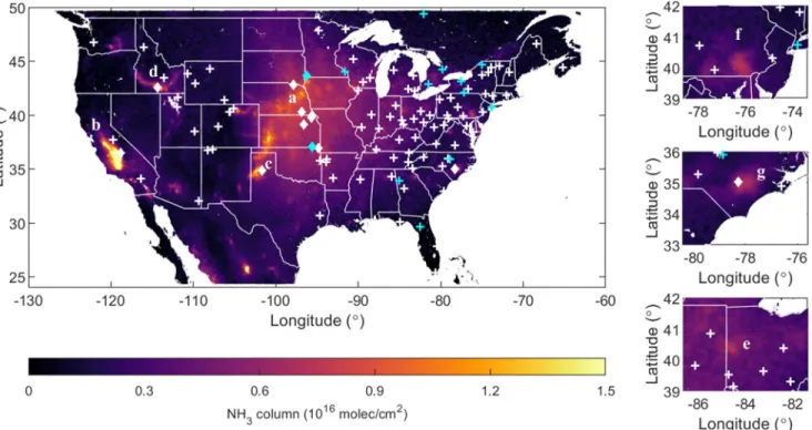
map. Annual maps were made by averaging the monthly maps in equal weights. Figure 1 shows 0.02° × 0.02° 2008–2017 oversampled NH3 column abundances derived from IASI observations along with the location of
AMoN sites in the CONUS. NH3 column abundances larger than the 95% (6.6 × 10¹⁵ mol cm−2) of the
10-year averaged level 3 map are defined as “hotspot” regions. This definition of hotspots differs from locating individual emission sources, though these are tightly correlated geographically due to the short lifetime of NH3. The 95% threshold concentration is not sensitive to the spatial resolution of the oversampling product
as coarser resolutions (0.05° × 0.05°, 0.1° × 0.1°) have similar 95% values (within ±5%).
By using the Hoshen–Kopelman algorithm to cluster adjacent grid points (Hoshen & Kopelman, 1976) above the 95% threshold, a total of 113 areal hotpots were identified (median area = 152 km2). Detailed
hot-spots locations and contours are shown in Figure S3. The square root of the median area yielded a charac-teristic hotspot length scale of 12 km (25th: 8 km, 75th: 24 km). The length scale was fairly insensitive to the oversampling product spatial resolution (0.05° × 0.05° = 13 km; 0.1° × 0.1° = 17 km), increasing slightly as expected due to the coarser grid resolution. The characteristic length scale was insensitive to the percentile as well (90th percentile = 5.3 × 10¹⁵ mol cm−2 yielded 11 km). In general, the characteristic length scale of
IASI NH3 hotspots is on the order of 10 km, indicating that coarser resolution (either in model or
observa-tions) may miss or average these hotspots into levels more typical of the background.
Figure 1. 2008–2017 averaged annual NH3 columns. Each active AMoN site (January 2020) is shown by a diamond “◊” (within 12 km of a hotspot) or a cross “+” symbol. Active AMoN sites are shown in white while inactive sites are shown in cyan. Labeled hotspots are: (a) Great Plains; (b) San Joaquin Valley; (c) Texas panhandle; (d) Snake River Valley; (e) west-central Ohio; (f) southeastern Pennsylvania, and (g) eastern North Carolina. For reference, the top 5% of annual NH3 columns (“hotspots”) correspond to 0.66 × 10¹⁶ mol cm−2.
The largest contiguous hotspot is in the central Great Plains (386,460 km2), and the San Joaquin Valley
hot-spot has the highest annual average column abundance (∼2.5 × 10¹⁶ mol cm−2). In terms of column-areal
weighting, the most important hotspots are the Great Plains, San Joaquin Valley, Texas panhandle, and the Snake River Valley. Although the eastern United States has lower column abundances and fewer hotspot re-gions than the western United States, PM2.5 formation in the eastern United States is more sensitive to NH3
than the western United States (Holt et al., 2015). Important hotspots in the eastern United States include west-central Ohio, southeastern Pennsylvania, and eastern North Carolina. The locations of these high NH3
columns are consistent with those previously reported in-situ observations, satellite analyses, AMoN net-work, and intensive agricultural activities (Clarisse et al., 2009; Nowak et al., 2012; Schiferl et al., 2016, 2014; Shephard et al., 2011; Van Damme et al., 2018).
Among the 121 AMoN sites (Figure 1), only 12 AMoN sites are located within 12 km of a hotspot region. AMoN site placement is prioritized to study nitrogen deposition in sensitive ecosystems, and additional sites near hotspots would be valuable for constraining emissions. The high-resolution satellite maps can guide site placement choices in the future, depending upon the ultimate science goal of a site (e.g., emis-sions vs. downstream deposition).
3.2. Ammonia Seasonality Across the CONUS
While annual maps of NH3 constrain the locations of emission sources, the intraannual patterns of NH3 are
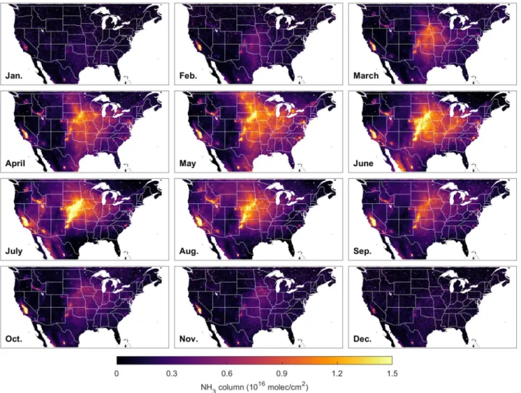
critical in evaluating aerosol formation and nitrogen deposition. Monthly maps at a moderate (30–100 km) spatial resolution average out many hotspots (Van Damme et al., 2014; Warner et al., 2016) and also provide limited information about how different areas evolve during the year. Figure 2 shows the 2008–2017 month-ly oversampled NH3 column concentrations over the CONUS. The general seasonality across the CONUS
shows high NH3 columns in spring/summer, and low NH3 concentrations in winter, consistent with past
studies (Henze et al., 2009; Paulot et al., 2014; Pinder et al., 2006). However, seasonal complexity exists due to regional differences in agricultural practices and climate. NH3 column maxima are observed in July or
August in the western United States, while maxima occur in May/June in the eastern United States (Fig-ure S4 in Supporting Information), in broad agreement with past work at coarser resolution (Van Damme et al., 2015).
The differences in monthly NH3 patterns are partially attributed to the dominant agricultural land use types
for each region. The western United States is dominated by pasture lands (USDA, 2017), and livestock waste volatilizes to produce NH3 with increasing temperatures (Gyldenkærne et al., 2005). The eastern United
States is featured by both pasture lands and croplands (USDA, 2017), and fertilizer and manure emissions lead to complex patterns across spring, summer, and fall. Note that the absolute differences between the monthly maxima and minima are large—on the order of 1016 mol cm−2—for most of the hotspot regions
(Figure S5).
To better understand the NH3 seasonal patterns beyond the monthly maxima, the IASI NH3 seasonality
was examined using k-means++ clustering (Arthur & Vassilvitskii, 2007; Forgy, 1965) of the monthly IASI NH3 columns. As an unsupervised learning algorithm, k-means++ groups observations so that the average
squared distance between data in the same cluster is minimized (Arthur & Vassilvitskii, 2007; Forgy, 1965). The advantage of applying k-means clustering is the lack of any a priori assumption of regional seasonality. The data define the geographical regions that have similar seasonality, and k-means++ is independently performed on different datasets. Monthly NH3 data were standardized to have a mean of 0 and a variance of
1. Therefore, the clustering is not affected by differences in the mean or variance but is instead based on the correlation among all standardized monthly concentrations (Zhang et al., 2016). Because the optimal num-ber of clusters is influenced by the underlying data and its patterns (Text S2), different optimal numbers of clusters were identified for each dataset (e.g., IASI, AMoN, model products).
Figure 3 shows the five geographic clusters (3a) identified for IASI NH3 and their seasonal dependencies
(3b). The area from Central Plains to the Great Lakes resides in a cluster with a broad, May peak, and a secondary shoulder in September (cluster 1). To the southeast of that area across the South and along the Gulf Coast (cluster 2), there is a peak in May, a local minimum in July, and a secondary smaller peak in Sep-tember/October. The interior western United States and adjacent high plains are subdivided into a narrower
and more pronounced peak in July for the southwest (cluster 3) or August for the northwest (cluster 4). New England, boreal Ontario, and Québec, and the maritime provinces (cluster 5) have relatively small variations all year round.
Springtime maxima are consistent with the timing of fertilizer application, particularly the later start of the growing season as one moves northward (USDA, 2010). Fall maxima or shoulders are also consistent with fall-based fertilizer application (Goebes et al., 2003; USDA, 2010). In contrast, the narrower, summer peaks of the western United States and high plains are more consistent with the volatilization of livestock waste that strongly correlates with maximum air temperatures (Gyldenkærne et al., 2005). Feedlots and croplands are often adjacent to one another, making definitive agricultural use classifications difficult. Most hotspot regions (67%) fall into the group with a broad peak from spring to early fall (cluster 1), indicating contributions from both livestock waste and fertilizer application. The remainder (32%) fall into one of the two clusters (3 and 4) with the sharp, summer peaks associated more closely with feedlot emissions. Besides agricultural emissions, biomass burning may also contribute to some of the seasonality (Bouwman et al., 1997), especially in summer in the western United States and agricultural burning in the fall in the southeastern United States (Bray et al., 2018; Giglio et al., 2006; Luo et al., 2015).
Figure 3 also shows CMAQ (c, d) and AM3 (e, f) modeled NH3 seasonality clusters using k-means++. The
clusters of CMAQ range from a strong summer peak (cluster i) to bimodal peaks in spring and fall (clus-ter ii). The differences between the CMAQ clusters fall within a narrower range than the differences among
the observed IASI clusters. All AM3 clusters show bimodal peaks in spring and fall with varying relative magnitudes. The geographic locations of the model NH3 clusters are far more random and less consistent
geographically with their neighbors than the IASI clusters (cf. Figure S6 shows CMAQ and AM3 seasonal-ities averaged to the IASI spatial clusters). Overall, the temporal evolution of the key clusters in AM3 and CMAQ shows agreement with IASI seasonality clusters, but the spatial patterns of the CMAQ and AM3 clusters strongly differ from those of IASI.
K-means++ clustering was also applied to the much smaller AMoN dataset. Three seasonality clusters were identified for 104 AMoN sites with sufficient (≥1-year record) seasonality measurements as shown in Figures 3g and 3h. Cluster γ, covering most of the eastern and Midwest U.S. sites, has a broad, single peak in June. Cluster α is featured by a peak in July and covers most regions in the western United States, in good agreement with the seasonal pattern classification with IASI. Cluster β shows a relatively insignificant sea-sonal variability except for a peak in November that is associated with seven sites and may be related to in-fluences from unidentified local sources. IASI and AMoN patterns are not perfectly matched, but both show the similar spatial clusters of seasonalities between the western and Midwestern/eastern United States and also are broadly consistent on the temporal patterns of NH3 seasonalities for each geographic area.
The patterns of IASI and modeled NH3 seasonality are affected by many factors such as emissions,
parti-tioning, and deposition. With respect to aerosol partiparti-tioning, gas-phase NH3 compromises much of the total
NHx in the warm season for both models (Figure S7 and S8). For deposition, only a small fraction (5–15%) Figure 3. IASI, CMAQ, AM3, and AMoN NH3 seasonality clusters map (a), (c), (e), and (g) and standardized NH3 concentrations for each cluster (b), (d), (f), and (h).
dry deposits within 15 km (Dennis et al., 2010; Miller et al., 2015). Indeed, Nair et al. (2019) showed that the modeled NH3 concentrations have a strong spatial dependence on NH3 emissions. However, away from
hot-spots and during the cold season, deposition and partitioning likely become more important contributors to the seasonal patterns than the underlying emission inventory. Because CMAQ and AM3 modeling results are based on state or county level emission inventory statistics, satellite observations constraints can be used to ameliorate the effects of these geopolitical boundaries on model output.
3.3. Seasonality of Hotspots: Comparison of Model and Observations
Case studies of IASI and AMoN NH3 seasonality over hotspots were examined and compared to CMAQ
and AM3 columns. Three 0.5° × 0.5° hotspot subregions were selected for comparison: (1) central Tulare County, California, the location of the highest IASI NH3 column (3.2 × 10¹⁶ mol cm−2) composed of 58%
cropland, 36% pastureland (USDA, 2017); (2) Cache County, Utah, the location of the highest annual AMoN NH3 surface concentrations (∼15 μg/m3) in the network (58% cropland, 37% pastureland, USDA, 2017);
and (3) Jo Daviess County, Illinois, a more cropland dominated hotspot (70% cropland, 14% pastureland) (USDA, 2017). Figures 4a, 4c, and 4e show the IASI oversampled NH3 column concentrations in Tulare,
Cache, and Jo Daviess counties, respectively. Figures 4b, 4d, and 4f show the corresponding seasonality comparison between IASI, CMAQ, AM3 NH3 columns, and AMoN NH3 surface concentration. While the
years included for AMoN, IASI, and model results differed amongst themselves at each site, the interannual variabilities are expected to be averaged out (Figure S9).
The three hotspots display distinctly different IASI NH3 seasonalities, showing that hotspot regions cannot
be treated identically. For Tulare County, IASI, AMoN, and CMAQ all show a broad summer peak in Tu-lare County, while AM3 shows a bimodal peak. For Cache County, all four patterns differ between AMoN, IASI, CMAQ, and AM3. AMoN measures a relatively flat pattern across the year, IASI shows a broad sum-mer peak, CMAQ has a stronger sumsum-mer peak, and AM3 has bimodal peaks. While IASI identifies Cache County as a hotspot, the AMoN site has the highest annual average in the CONUS. However, this AMoN site is only ∼100 m away from feedlots, a distance in which concentrations are strongly enhanced relative to background levels (Golston et al., 2020; Miller et al., 2015). There are also intrinsic differences between a surface concentration and column amount that complicate comparisons between IASI and AMoN (e.g., boundary layer height). Meanwhile, Jo Daviess County exhibits a broad spring peak in IASI, but a bimodal structure in AMoN and AM3. IASI NH3 columns over hotspot regions allow one to test the relevant model
parameters that impact seasonality (e.g., partitioning, emissions, deposition, transport).
4. Implications
Ammonia columns near source regions are very localized (∼12 km scale) and with strong spatial gradients. Because NH3 hotspots have a strong influence on the air quality and nitrogen deposition in nearby regions
(Benedict et al., 2013), there is an urgent need to understand processes such as the underlying spatial pat-tern of emission inventories, deposition, transport, and partitioning at these same scales. Satellite data may help improve future site placement depending upon the desired objective (e.g., investigating hotspots emis-sions or characterizing downwind deposition). Ultimately, the differences in spatial and temporal scales be-tween satellite observations (an instantaneous volume) and AMoN (two-week point measurement) require careful attention to many factors for robust comparisons (Kharol et al., 2018).
At monthly scales, the high-resolution NH3 maps provide improved, observational-based means to help
constrain NH3 seasonality for improved regional scale modeling of PM2.5 and deposition. The differences
be-tween satellite and modeled NH3 seasonal patterns, especially for the global emission inventories developed
for CMIP6, further demonstrate the importance of evaluating modeled NH3 with satellite measurements.
Simply using the annual averages with a priori seasonalities applied is not accurate. To this end, recent work by Chen et al. (2020) is promising where IASI NH3 is inverted at 36-km resolution for April, July,
and October with much different emissions spatially and temporally. Accurate modeling of boundary layer height, vertical profiles of temperature, humidity, and NH3 within the boundary layer, aerosol partitioning,
and chemical lifetime are all needed to fully transform these column maps into accurate spatiotemporal emission inventories. Finally, additional validations (Guo et al., 2021) of satellite-derived NH3 columns
Figure 4. Comparison of NH3 seasonality in hotspots regions. Panels (a), (c), and (e) are the annual averaged IASI oversampled NH3 column concentrations. The bold black dashed box indicates the selected hotspot regions. The black cross shows the nearby AMoN site. Black dashed lines represent AM3 grid boxes, and white dots represent the center of CMAQ grids. (b), (d), and (f) are the NH3 seasonality derived from the IASI oversampling NH3 column, CMAQ, and AM3 modeled NH3 columns (left axis), and AMoN NH3 concentration (right axis). Map data from Google Earth.
are also needed to reduce biases at these scales (especially for conditions of temperature inversions during winter and in valleys).
Data Availability Statement
The monthly resolved 0.02° × 0.02° IASI oversampling data, IASI data animations, and kmz file of annual data are available on the persistent URL: https://dataspace.princeton.edu/handle/88435/dsp018s45qc83f, DOI: https://doi.org/10.34770/J1Q6-2Y79.
References
Arthur, D., & Vassilvitskii, S. (2007). K-means++: The advantages of careful seeding. Paper presented atproceedings of the eighteenth
annual ACM-SIAM symposium on discrete algorithms (SODA '07). New Orleans, LA: Society for Industrial and Applied Mathematics.
Bash, J. O., Cooter, E. J., Dennis, R. L., Walker, J. T., & Pleim, J. E. (2013). Evaluation of a regional air-quality model with bidirectional NH3
exchange coupled to an agroecosystem model. Biogeosciences, 10(3), 1635–1645. https://doi.org/10.5194/bg-10-1635-2013
Battye, W. H., Bray, C. D., Aneja, V. P., Tong, D., Lee, P., & Tang, Y. (2019). Evaluating ammonia (NH3) predictions in the NOAA NAQFC for
Eastern North Carolina using ground level and satellite measurements. Journal of Geophysical Research: Atmospheres, 124, 8242–8259.
https://doi.org/10.1029/2018JD029990
Benedict, K. B., Day, D., Schwandner, F. M., Kreidenweis, S. M., Schichtel, B., Malm, W. C., & Collett, J. L. (2013). Observations of atmos-pheric reactive nitrogen species in Rocky Mountain National Park and across northern Colorado. Atmosatmos-pheric Environment, 64, 66–76.
https://doi.org/10.1016/j.atmosenv.2012.08.066
Bouwman, A. F., Lee, D. S., Asman, W. A. H., Dentener, F. J., Van Der Hoek, K. W., & Olivier, J. G. J. (1997). A global high-resolution emis-sion inventory for ammonia. Global Biogeochemical Cycles, 11(4), 561–587. https://doi.org/10.1029/97GB02266
Bray, C. D., Battye, W., Aneja, V. P., Tong, D. Q., Lee, P., & Tang, Y. (2018). Ammonia emissions from biomass burning in the continental United States. Atmospheric Environment, 187, 50–61. https://doi.org/10.1016/j.atmosenv.2018.05.052
Cao, H., Henze, D. K., Shephard, M. W., Dammers, E., Cady-Pereira, K., Alvarado, M., et al. (2020). Inverse modeling of NH3 sources using
CrIS remote sensing measurements. Environmental Research Letters, 15(10), 104082. https://doi.org/10.1088/1748-9326/abb5cc
Chen, Y., Shen, H., Kaiser, J., Hu, Y., Capps, S. L., Zhao, S., et al. (2021). High-resolution hybrid inversion of IASI ammonia columns to constrain U.S. Ammonia emissions using the CMAQ Adjoint model. Atmospheric Chemistry and Physics, 21, 2067–2082. https://doi. org/10.5194/acp-21-2067-2021
Clarisse, L., Clerbaux, C., Dentener, F., Hurtmans, D., & Coheur, P.-F. (2009). Global ammonia distribution derived from infrared satellite observations. Nature Geoscience, 2(7), 479–483. https://doi.org/10.1038/ngeo551
Clarisse, L., Shephard, M. W., Dentener, F., Hurtmans, D., Cady-Pereira, K., Karagulian, F., et al. (2010). Satellite monitoring of ammonia: A case study of the San Joaquin Valley. Journal of Geophysical Research, 115, D13302. https://doi.org/10.1029/2009JD013291
Clarisse, L., Van Damme, M., Clerbaux, C., & Coheur, P. F. (2019). Tracking down global NH3 point sources with wind-adjusted
superres-olution. Atmospheric Measurement Techniques, 12(10), 5457–5473. https://doi.org/10.5194/amt-12-5457-2019
Dammers, E., McLinden, C. A., Griffin, D., Shephard, M. W., Van Der Graaf, S., & Lutsch, E., (2019). NH3 emissions from large point
sources derived from CrIS and IASI satellite observations. Atmospheric Chemistry and Physics, 19(19), 12261–12293. http://dx.doi. org/10.5194/acp-19-12261-2019
Dennis, R. L., Mathur, R., Pleim, J. E., & Walker, J. T. (2010). Fate of ammonia emissions at the local to regional scale as simulated by the Community Multiscale Air Quality model. Atmospheric Pollution Research, 1(4), 207–214. https://doi.org/10.5094/APR.2010.027
Donner, L. J., Wyman, B. L., Hemler, R. S., Horowitz, L. W., Ming, Y., Zhao, M., et al. (2011). The dynamical core, physical parameteri-zations, and basic simulation characteristics of the atmospheric component AM3 of the GFDL global coupled model CM3. Journal of
Climate, 24(13), 3484–3519. https://doi.org/10.1175/2011JCLI3955.1
Fehsenfeld, F. C., Huey, L. G., Leibrock, E., Dissly, R., Williams, E., Ryerson, T. B., et al. (2002). Results from an informal intercomparison of ammonia measurement techniques. Journal of Geophysical Research, 107(D24), 4812. https://doi.org/10.1029/2001JD001327
Forgy, E. (1965). Cluster analysis of multivariate data: Efficiency versus interpretability of classifications. Biometrics, 21, 768–869. Friedrich, R., & Reis, S. (2004). Emissions of air pollutants: Measurements, calculations and uncertainties. Berlin Heidelberg, NY: Springer. Giglio, L., Csiszar, I., & Justice, C. O. (2006). Global distribution and seasonality of active fires as observed with the Terra and Aqua Mod-erate Resolution Imaging Spectroradiometer (MODIS) sensors. Journal of Geophysical Research, 111, G02016. 10.1029/2005JG000142
Gilliland, A. B. (2003). Seasonal NH3 emission estimates for the eastern United States based on ammonium wet concentrations and an
inverse modeling method. Journal of Geophysical Research, 108(D15), 4477. https://doi.org/10.1029/2002JD003063
Gilliland, A. B., Wyat Appel, K., Pinder, R. W., & Dennis, R. L. (2006). Seasonal NH3 emissions for the continental united states: Inverse
model estimation and evaluation. Atmospheric Environment, 40(26), 4986–4998. https://doi.org/10.1016/j.atmosenv.2005.12.066
Goebes, M. D., Strader, R., & Davidson, C. (2003). An ammonia emission inventory for fertilizer application in the United States.
Atmos-pheric Environment, 37(18), 2539–2550. https://doi.org/10.1016/S1352-2310(03)00129-8
Golston, L. M., Pan, D., Sun, K., Tao, L., Zondlo, M. A., Eilerman, S. J., et al. (2020). Variability of ammonia and methane emissions from animal feeding operations in northeastern Colorado. Environmental Science and Technology, 54, 11015–11024. https://doi.org/10.1021/ acs.est.0c00301
Guo, X., Wang, R., Pan, D., Zondlo, M. A., Clarisse, L., Van Damme, M., et al. (2021). Validation of IASI satellite ammonia observa-tions at the pixel scale using in-situ vertical profiles. Journal of Geophysical Research: Atmospheres, 126, e2020JD033475. https://doi. org/10.1029/2020JD033475
Gyldenkærne, S., Skjøth, C. A., Hertel, O., & Ellermann, T. (2005). A dynamical ammonia emission parameterization for use in air pollu-tion models. Journal of Geophysical Research, 110, D07108. https://doi.org/10.1029/2004JD005459
Hauglustaine, D. A., Balkanski, Y., & Schulz, M. (2014). A global model simulation of present and future nitrate aerosols and their direct radiative forcing of climate. Atmospheric Chemistry and Physics, 14(20), 11031–11063. https://doi.org/10.5194/acp-14-11031-2014
Heald, C. L., Collett, J. L., Lee, T., Benedict, K. B., Schwandner, F. M., Li, Y., et al. (2012). Atmospheric ammonia and particulate inorganic nitrogen over the United States. Atmospheric Chemistry and Physics, 12(21), 10295–10312. https://doi.org/10.5194/acp-12-10295-2012
Acknowledgments
The authors acknowledge support from the NASA Health and Air Quality Applied Sciences team (NASA NNX16AQ90G). X. Guo acknowledges the support from NASA Earth and Space Science Fellowship (80NSS-C17K0377). Part of the research at the ULB has been supported by the IASI Flow Prodex arrangement (ESA-BEL-SPO). L. Clarisse and M.V. Damme were supported by the F.R.S.-FNRS. Ammonia Monitoring Network/NADP is acknowledged for providing the NH3
AMON data. The views expressed in this manuscript are those of the authors alone and do not necessarily reflect the views and policies of the U.S. Environ-mental Protection Agency.
Henze, D. K., Seinfeld, J. H., & Shindell, D. T. (2009). Inverse modeling and mapping US air quality influences of inorganic PM 2.5 precursor emissions using the adjoint of GEOS-Chem. Atmospheric Chemistry and Physics, 9(16), 5877–5903. https://doi.org/10.5194/ acp-9-5877-2009
Hill, J., Goodkind, A., Tessum, C., Thakrar, S., Tilman, D., Polasky, S., et al. (2019). Air-quality-related health damages of maize. Nature
Sustainability, 2(5), 397–403. https://doi.org/10.1038/s41893-019-0261-y
Hoesly, R. M., Smith, S. J., Feng, L., Klimont, Z., Janssens-Maenhout, G., Pitkanen, T., et al. (2018). Historical (1750-2014) anthropogenic emissions of reactive gases and aerosols from the Community Emissions Data System (CEDS). Geoscientific Model Development, 11(1), 369–408. https://doi.org/10.5194/gmd-11-369-2018
Holt, J., Selin, N. E., & Solomon, S. (2015). Changes in inorganic fine particulate matter sensitivities to precursors due to large-scale us emissions reductions. Environmental Science and Technology, 49(8), 4834–4841. https://doi.org/10.1021/acs.est.5b00008
Hoshen, J., & Kopelman, R. (1976). Percolation and cluster distribution. I. Cluster multiple labeling technique and critical concentration algorithm. Physical Review B, 14, 3438. https://doi.org/10.1103/PhysRevB.14.3438
Kelly, J. T., Baker, K. R., Nolte, C. G., Napelenok, S. L., Keene, W. C., & Pszenny, A. A. P. (2016). Simulating the phase partitioning of NH3, HNO3, and HCl with size-resolved particles over northern Colorado in winter. Atmospheric Environment, 131, 67–77. https://doi.
org/10.1016/j.atmosenv.2016.01.049
Kelly, J. T., Baker, K. R., Nowak, J. B., Murphy, J. G., Markovic, M. Z., Vandenboer, T. C., et al. (2014). Fine-scale simulation of ammonium and nitrate over the south coast air basin and San Joaquin valley of California during CalNex-2010. Journal of Geophysical Research:
Atmospheres, 119, 3600–3614. https://doi.org/10.1002/2013JD021290
Kelly, J. T., Koplitz, S. N., Baker, K. R., Holder, A. L., Pye, H. O. T., Murphy, B. N., et al. (2019). Assessing PM2.5 model performance for the
conterminous U.S. with comparison to model performance statistics from 2007-2015. Atmospheric Environment, 214, 116872. https:// doi.org/10.1016/j.atmosenv.2019.116872
Kelly, J. T., Parworth, C. L., Zhang, Q., Miller, D. J., Sun, K., Zondlo, M. A., et al. (2018). Modeling NH4NO3 over the San Joaquin
Valley during the 2013 DISCOVER-AQ campaign. Journal of Geophysical Research: Atmospheres, 123, 4727–4745. https://doi. org/10.1029/2018JD028290
Kharol, S. K., Shephard, M. W., McLinden, C. A., Zhang, L., Sioris, C. E., O’Brien, J. M., et al. (2018). Dry deposition of reactive nitrogen from satellite observations of ammonia and nitrogen dioxide over North America. Geophysical Research Letters, 45, 1157–1166. https:// doi.org/10.1002/2017GL075832
Li, Y., Schichtel, B. A., Walker, J. T., Schwede, D. B., Chen, X., Lehmann, C. M. B., et al. (2016). Increasing importance of deposition of re-duced nitrogen in the United States. Proceedings of the National Academy of Sciences of the United States of America, 113(21), 5874–5879. Luo, M., Shephard, M. W., Cady-Pereira, K. E., Henze, D. K., Zhu, L., Bash, J. O., et al. (2015). Satellite observations of tropospheric ammo-nia and carbon monoxide: Global distributions, regional correlations and comparisons to model simulations. Atmospheric Environment,
106, 262–277. https://doi.org/10.1016/j.atmosenv.2015.02.007
Malm, W. C., Schichtel, B. A., Pitchford, M. L., Ashbaugh, L. L., & Eldred, R. A. (2004). Spatial and monthly trends in speciated fine particle concentration in the United States. Journal of Geophysical Research, 109, D03306. https://doi.org/10.1029/2003JD003739
Massad, R. S., Nemitz, E., & Sutton, M. A. (2010). Review and parameterisation of bi-directional ammonia exchange between vegetation and the atmosphere. Atmospheric Chemistry and Physics, 10(21), 10359–10386. https://doi.org/10.5194/acp-10-10359-2010
Miller, D. J., Sun, K., Tao, L., Pan, D., Zondlo, M. A., Nowak, J. B., et al. (2015). Ammonia and methane dairy emission plumes in the San Joaquin valley of California from individual feedlot to regional scales. Journal of Geophysical Research: Atmospheres, 120, 9718–9738.
https://doi.org/10.1002/2015JD023241
Naik, V., Voulgarakis, A., Fiore, A. M., Horowitz, L. W., Lamarque, J. F., Lin, M., et al. (2013). Preindustrial to present-day changes in tropospheric hydroxyl radical and methane lifetime from the Atmospheric Chemistry and Climate Model Intercomparison Project (ACCMIP). Atmospheric Chemistry and Physics, 13(10), 5277–5298. https://doi.org/10.5194/acp-13-5277-2013
Nair, A. A., Yu, F., & Luo, G. (2019). Spatioseasonal variations of atmospheric ammonia concentrations over the United States: Comprehensive model-observation comparison. Journal of Geophysical Research: Atmospheres, 124, 6571–6582. https://doi.org/10.1029/2018JD030057
NADP, National Atmospheric Deposition Program (NRSP-3). (2020). NADP program office. Madison, WI: Wisconsin State Laboratory of Hygiene. Retrieved from http://nadp.slh.wisc.edu/AMoN/
Nowak, J. B., Neuman, J. A., Bahreini, R., Middlebrook, A. M., Holloway, J. S., McKeen, S. A., et al. (2012). Ammonia sources in the Cal-ifornia South Coast Air Basin and their impact on ammonium nitrate formation. Geophysical Research Letters, 39, L07804. https://doi. org/10.1029/2012GL051197
Paulot, F., Ginoux, P., Cooke, W. F., Donner, L. J., Fan, S., Lin, M. Y., et al. (2016). Sensitivity of nitrate aerosols to ammonia emissions and to nitrate chemistry: Implications for present and future nitrate optical depth. Atmospheric Chemistry and Physics, 16(3), 1459–1477.
https://doi.org/10.5194/acp-16-1459-2016
Paulot, F., & Jacob, D. J. (2014). Hidden cost of U.S. agricultural exports: Particulate matter from ammonia emissions. Environmental
Sci-ence and Technology, 48(2), 903–908. https://doi.org/10.1021/es4034793
Paulot, F., Jacob, D. J., Pinder, R. W., Bash, J. O., Travis, K., & Henze, D. K. (2014). Ammonia emissions in the United States, European Union, and China derived by high-resolution inversion of ammonium wet deposition data: Interpretation with a new agricultural emis-sions inventory (MASAGE_NH3). Journal of Geophysical Research: Atmospheres, 119, 4343–4364. https://doi.org/10.1002/2013JD021130
Paulot, F., Paynter, D., Ginoux, P., Naik, V., & Horowitz, L. W. (2018). Changes in the aerosol direct radiative forcing from 2001 to 2015: Observational constraints and regional mechanisms. Atmospheric Chemistry and Physics, 18(17), 13265–13281. https://doi.org/10.5194/ acp-18-13265-2018
Paulot, F., Paynter, D., Ginoux, P., Naik, V., Whitburn, S., Van Damme, M., et al. (2017). Gas-aerosol partitioning of ammonia in biomass burning plumes: Implications for the interpretation of spaceborne observations of ammonia and the radiative forcing of ammonium nitrate. Geophysical Research Letters, 44, 8084–8093. https://doi.org/10.1002/2017GL074215
Phoenix, G. K., Hicks, W. K., Cinderby, S., Kuylenstierna, J. C. I., Stock, W. D., Dentener, F. J., et al. (2006). Atmospheric nitrogen deposition in world biodiversity hotspots: The need for a greater global perspective in assessing N deposition impacts. Global Change Biology, 12(3), 470–476. https://doi.org/10.1111/j.1365-2486.2006.01104.x
Pinder, R. W., Adams, P. J., Pandis, S. N., & Gilliland, A. B. (2006). Temporally resolved ammonia emission inventories: Current estimates, evaluation tools, and measurement needs. Journal of Geophysical Research, 111, D16310. https://doi.org/10.1029/2005JD006603
Puchalski, M. A., Rogers, C. M., Baumgardner, R., Mishoe, K. P., Price, G., Smith, M. J., et al. (2015). A statistical comparison of active and passive ammonia measurements collected at Clean Air Status and Trends Network (CASTNET) sites. Environmental Sciences: Processes
Reis, S., Pinder, R. W., Zhang, M., Lijie, G., & Sutton, M. A. (2009). Reactive nitrogen in atmospheric emission inventories. Atmospheric
Chemistry and Physics, 9, 7657–7677. https://doi.org/10.5194/acp-9-7657-2009
Schiferl, L. D., Heald, C. L., Damme, M. V., Clarisse, L., Clerbaux, C., Coheur, P., et al. (2016). Interannual variability of ammonia concen-trations over the United States: Sources and implications. Atmospheric Chemistry and Physics, 16, 12305–12328. https://doi.org/10.5194/ acp-16-12305-2016
Schiferl, L. D., Heald, C. L., Nowak, J. B., Holloway, J. S., Neuman, J. A., Bahreini, R., et al. (2014). An investigation of ammonia and in-organic particulate matter in California during the CalNex campaign. Journal of Geophysical Research: Atmospheres, 119, 1883–1902.
https://doi.org/10.1002/2013JD020765
Shephard, M. W., & Cady-Pereira, K. E. (2015). Cross-track Infrared Sounder (CrIS) satellite observations of tropospheric ammonia.
Atmos-pheric Measurement Techniques, 8(3), 1323–1336. https://doi.org/10.5194/amt-8-1323-2015
Shephard, M. W., Cady-Pereira, K. E., Luo, M., Henze, D. K., Pinder, R. W., Walker, J. T., et al. (2011). TES ammonia retrieval strategy and global observations of the spatial and seasonal variability of ammonia. Atmospheric Chemistry and Physics, 11(20), 10743–10763. https:// doi.org/10.5194/acp-11-10743-2011
Shephard, M. W., Dammers, E., Cady-Pereira, K. E., Kharol, S. K., Thompson, J., Gainariu-Matz, et al. (2020). Ammonia measurements from space with the Cross-track Infrared Sounder: Characteristics and applications. Atmospheric Chemistry and Physic, 20, 2277–2302.
https://doi.org/10.5194/acp-20-2277-2020
Sun, K., Zhu, L., Cady-Pereira, K., Chan Miller, C., Chance, K., Clarisse, L., et al. (2018). A physics-based approach to oversample multi-sat-ellite, multispecies observations to a common grid. Atmospheric Measurement Techniques, 11(12), 6679–6701. https://doi.org/10.5194/ amt-11-6679-2018
USDA National Agricultural Statistics Service. (2010). Field crops usual planting and harvesting dates. Retrieved from https://www.nass. usda.gov/Publications/Todays_Reports/reports/fcdate10.pdf
USDA National Agricultural Statistics Service. (2017). Census of agriculture. Retrieved from https://www.nass.usda.gov/AgCensus
USEPA. (2018). Bayesian space-time downscaling fusion model (downscaler)-derived estimates of air quality for 2014. Research Triangle Park, NC: U.S. Environmental Protection Agency, Office of Air Quality Planning and Standards. EPA-454/R-18-008. Retrieved from
https://www.epa.gov/hesc/rsig-related-downloadable-data-files
Van Damme, M., Clarisse, L., Heald, C. L., Hurtmans, D., Ngadi, Y., Clerbaux, C., et al. (2014). Global distributions, time series and error characterization of atmospheric ammonia (NH3) from IASI satellite observations. Atmospheric Chemistry and Physics, 14(6), 2905–2922.
https://doi.org/10.5194/acp-14-2905-2014
Van Damme, M., Clarisse, L., Whitburn, S., Hadji-Lazaro, J., Hurtmans, D., Clerbaux, C., & Coheur, P. F. (2018). Industrial and agricultural ammonia point sources exposed. Nature, 564(7734), 99–103. https://doi.org/10.1038/s41586-018-0747-1
Van Damme, M., Erisman, J. W., Clarisse, L., Dammers, E., Whitburn, S., Clerbaux, C., et al. (2015). Worldwide spatiotemporal at-mospheric ammonia (NH3) columns variability revealed by satellite. Geophysical Research Letters, 42, 8660–8668. https://doi.
org/10.1002/2015GL065496
Van Damme, M., Whitburn, S., Clarisse, L., Clerbaux, C., Hurtmans, D., & Coheur, P. F. (2017). Version 2 of the IASI NH3 neural
net-work retrieval algorithm: Near-real-time and reanalysed datasets. Atmospheric Measurement Techniques, 10(12), 4905–4914. https://doi. org/10.5194/amt-10-4905-2017
von Bobrutzki, K., Braban, C. F., Famulari, D., Jones, S. K., Blackall, T., Smith, T. E. L., et al. (2010). Field inter-comparison of eleven atmos-pheric ammonia measurement techniques. Atmosatmos-pheric Measurement Techniques, 3, 91–112. https://doi.org/10.5194/amt-3-91-2010
Walker, J. M., Philip, S., Martin, R. V., & Seinfeld, J. H. (2012). Simulation of nitrate, sulfate, and ammonium aerosols over the United States. Atmospheric Chemistry and Physics, 12(22), 11213–11227. https://doi.org/10.5194/acp-12-11213-2012
Warner, J. X., Dickerson, R. R., Wei, Z., Strow, L. L., Wang, Y., & Liang, Q. (2017). Increased atmospheric ammonia over the world’s major agricultural areas detected from space. Geophysical Research Letters, 44, 2875–2884. https://doi.org/10.1002/2016GL072305
Warner, J. X., Wei, Z., Larrabee Strow, L., Dickerson, R. R., & Nowak, J. B. (2016). The global tropospheric ammonia distribution as seen in the 13-year AIRS measurement record. Atmospheric Chemistry and Physics, 16(8), 5467–5479. https://doi.org/10.5194/acp-16-5467-2016
Whitburn, S., Van Damme, M., Clarisse, L., Bauduin, S., Heald, C. L., Hurtmans, D., et al. (2016). A flexible and robust neural network IASI-NH3. Journal of Geophysical Research: Atmospheres, 121, 6581–6599. https://doi.org/10.1002/2016JD024828
Yao, X., & Zhang, L. (2016). Trends in atmospheric ammonia at urban, rural, and remote sites across North America. Atmospheric
Chem-istry and Physics, 16(17), 11465–11475. https://doi.org/10.5194/acp-16-11465-2016
Zhang, Y., Moges, S., & Block, P. (2016). Optimal cluster analysis for objective regionalization of seasonal precipitation in regions of high spatial-temporal variability: Application to Western Ethiopia. Journal of Climate, 29(10), 3697–3717. https://doi.org/10.1175/ JCLI-D-15-0582.1
Zhu, L., Henze, D. K., Cady-Pereira, K. E., Shephard, M. W., Luo, M., Pinder, R. W., et al. (2013). Constraining U.S. ammonia emissions using TES remote sensing observations and the GEOS-Chem adjoint model. Journal of Geophysical Research: Atmospheres, 118, 3355– 3368. https://doi.org/10.1002/jgrd.50166