Diagnosing the variability in temperature and velocity in the Middle Atlantic Bight

(1)

Diagnosing the variability in temperature and velocity in the

Middle Atlantic Bight

by

Jacob Samuel Tse Forsyth

B.A., Bowdoin College (2015)

Submitted to the Department of Earth, Atmospheric, and Planetery Sciences in partial fulfillment of the requirements for the degree of

Doctor of Philosophy at the

MASSACHUSETTS INSTITUTE OF TECHNOLOGY and the

WOODS HOLE OCEANOGRAPHIC INSTITUTION February 2021

c

The author hereby grants to MIT and WHOI permission to reproduce and to distribute publicly paper and electronic copies of this thesis document in whole or in part in any

medium now known or hereafter created.

Author . . . . Joint Program in Oceanography/Applied Ocean Science & Engineering Massachusetts Institute of Technology & Woods Hole Oceanographic Institution October 29, 2020 Certified by . . . . Magdalena Andres Associate Scientist Woods Hole Oceanographic Institution Thesis Supervisor Certified by . . . . Glen Gawarkiewicz Senior Scientist Woods Hole Oceanographic Institution Thesis Supervisor Accepted by . . . .

Glenn Flierl Chair, Joint Committee for Physical Oceanography Massachusetts Institute of Technology & Woods Hole Oceanographic Institution

(2)

(3)

Diagnosing the variability in temperature and velocity in the Middle Atlantic Bight

by

Jacob Samuel Tse Forsyth

Submitted to the Department of Earth, Atmospheric, and Planetery Sciences on October 29, 2020, in partial fulfillment of the

requirements for the degree of Doctor of Philosophy

Abstract

Observations of hydrographic and dynamical properties on the Middle Atlantic Bight shelf docu-ment strong variability at time scales spanning events that last a few days to century long trends. This thesis studies individual processes which impact shelf temperature and velocity structure, and quantifies the mean velocity conditions at the shelf break. Chapter 2 uses model output to study the dynamics that lead to the breakdown of summertime thermal stratification, and how the processes which reduce stratification vary from year to year. In summer, the atmosphere heats the surface of the ocean, leading to strong thermal stratification with warm water overlying cool water. During fall, strong storm events with downwelling-favorable winds are found to be the primary process by which stratification is reduced. The timing of these events and the associated destratification varies from year to year. In Chapter 3, the velocity structure of the New Jersey shelf break is examine, with a focus on the Shelfbreak Jet. Using 25 years of velocity measurements, mean velocity sections of the Shelfbreak Jet are created in both Eulerian and stream coordinate frameworks. The jet exhibits strong seasonal variability, with maximum velocities observed in spring and minimum velocities in summer. Evidence is found that Warm Core Rings, originating from the Gulf Stream and passing through the Slope Sea adjacent to the New Jersey shelf, tend to shift the Shelfbreak Jet onshore of its mean position or entirely shutdown the Shelfbreak Jet’s flow. At interannual timescales, variabil-ity in the Shelfbreak Jet velocvariabil-ity is correlated with the temperature on the New Jersey Shelf, with temperature lagging by about 2 months. Chapter 4 focuses on the impact of Warm Core Rings on the velocity and temperature structure on the New Jersey shelf. Warm Core Rings that have higher azimuthal velocities and whose cores approach closer to the shelf are found to exert greater influence on the shelf’s along-shelf velocities, with the fastest and closest rings reversing the direction of flow at the shelf break. Warm Core Rings are also observed to exert long-lasting impacts on the shelf temperature, with faster rings cooling the shelf and slower rings warming the shelf. Seasonal changes in thermal stratification strongly affect how rings alter the shelf temperature. Rings in summer tend to cool the shelf, and rings throughout the rest of the year generally warm the shelf.

Thesis Supervisor: Magdalena Andres Title: Associate Scientist

Woods Hole Oceanographic Institution

Thesis Supervisor: Glen Gawarkiewicz Title: Senior Scientist

(4)

(5)

Acknowledgments

The completion of this thesis would not have been possible without massive help from a whole village of people.

First and foremost, I cannot imagine how I would have finished this program without my partner Jennifer Kenyon. She supported and assisted me through the stresses of qualifying exams, late nights finishing up manuscripts, and managing to actually finish writing this thesis on time. Without her, and our dog Ruby, this whole process would have been a lot more difficult.

I never would have realized my love for science research without my parents finding every op-portunity for me to experiment in my budding interest in science in middle school and high school. They have always enabled me to find what made me happiest and most fulfilled in my education and now professional career.

I need to thank my advisors Magdalena Andres and Glen Gawarkiewicz for introducing me to oceanographic research when I was a summer student fellow in such a way that I decided to commit these last 5 years to research. From teaching me the basics of coding, to placing me in charge of a scientific cruise, I have grown and learned so much from these two. They both have pushed me to take every opportunity that I could, and have made sure that I was always doing research that I enjoyed working on every day.

My friends made surviving the dark winters in Woods Hole warm, and the summers full of fun. Days of hanging out, fishing, board games, video games, pot lucks, and sports have made these years so enjoyable. Special thanks to the CARPO softball team (and all the other softball teams that let me play), as well as the WHOI lunch time soccer crew.

Thank you to office mates that have had to endure my presence on a daily basis. The support of my office mates through classes and qualifying exams was necessary. A special acknowledgement to Joleen Heiderich who answered countless stupid questions and allowed me to bounce many ideas off her for more than 6 years of sharing an office together.

Two of the three chapters are reliant on the CMV Oleander data. I am greatly appreciative of Charlie Flagg, Thomas Rossby, Kathy Donohue, Sandy Fontana, Ruth Curry, and everyone else that helps run and maintain the scientific equipment, as well as Bermuda Container Lines for allowing scientific instruments to be built into their ship.

There are many scientists who have provided great support and advice to this work, especially my committee members.

Everyone within the Academic Programs Office were always so helpful, great to work with, and ready to just have a little chat.

Thank you to the National Science Foundation and Academic Programs Office for funding my research. This research was funded under WHOI Academic Programs Endowed Funds, NSF #OCE-1634094, and NSF #OCE-1924041.

(6)

(7)

List of Figures

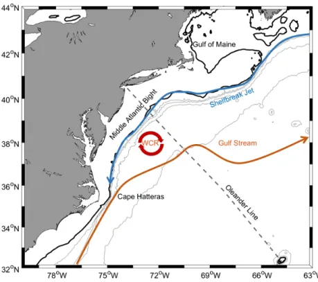
1-1 Map of the Northwest Atlantic with key regions and features labelled. . . 22

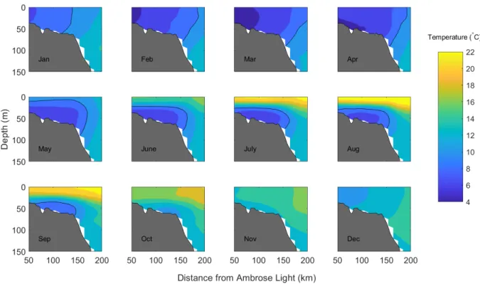
1-2 Monthly climatologies from 1977–2018 of temperatures on the MAB shelf from the

CMV Oleander XBTs. The black contour indicates the 10∘C. Updated figure from Forsyth

et al. (2015). . . 24

1-3 Time series of spatially and 12 month moving averaged temperatures on the MAB

shelf from Oleander XBTs. Linear trends are calculated: 40 year trend (grey dashed

line), 1977–2001 trend (yellow dashed line), and 2001–2017 (purple dashed line). . . . 25

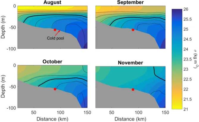
2-1 Transects of potential density (colored shading) for different climatological months

from the MABGOM model output. The transect shown here is along ”Model Transect”

from Figure 2-3. Contours of potential temperature are plotted every 2∘C in black,

the bold line marks the 14∘C contour. The red circle is at the 55-m isobath, within

the cold pool. . . 32

2-2 Map of the MABGOM model domain. The continental shelf is highlighted in blue and

bounded by the smoothed 80-m isobath (black bold line). The 1000, 2000, and

4000-m isobaths in the 4000-model are countoured in grey. The red line 4000-marks the boundary of

the model. The purple box shows the domain of Figure 2-3. . . 36

2-3 A zoomed in section of Figure 2-2 (marked as the purple box). Here we also identify

the model transect along which output is extracted (red line) and the 55-m isobath

on this transect (red circle). The SW06 mapped transect is plotted as a purple line

(12)

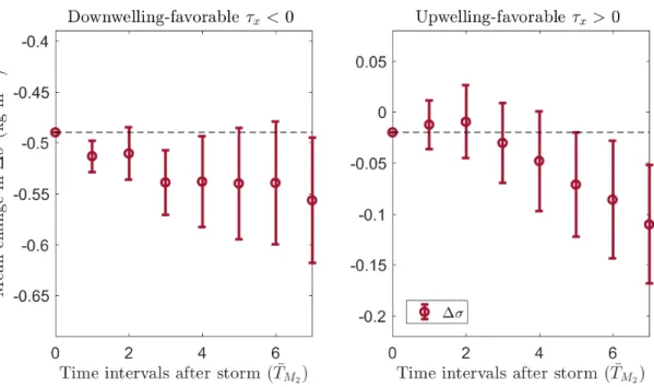
2-4 The mean change of ∆𝜎 as a function of the number of MABGOM model time

in-tervals after a storm is over with standard errors plotted as error bars. The means

are only calculated for storms which did not have another storm within the

restrati-fication period considered (8 time intervals of 12.42 hours after a storm has ended).

Left panel only considers downwelling-favorable storms, and the right column only

considers upwelling-favorable storms. Black dashed line shows the mean change in

stratification by the storms considered. Both y-axes span the same range. Negative

values represent destratification. . . 40

2-5 Interannual variability of the initial fall stratification from the MABGOM model

(thick black line associated with the left y axis) and the interannual variability of the

destratification point (right y axis) for the MABGOM model (red), the PWP HEAT

(blue), and PWP ALL (purple). PWP WIND never reaches the destratification point

by the end of each year and thus is not shown. . . 41

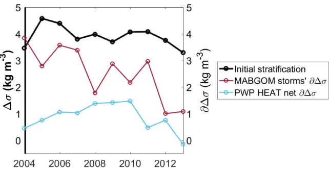
2-6 Interannual variability of the initial fall stratification from the MAGBOM model

(thick black line associated with the left y axis) and the interannual variability of how

storms in the MABGOM model impact stratification (red) and how heat fluxes (PWP

HEAT) impact stratification (teal). For PWP HEAT the net change in ∆𝜎 from initial

fall stratification until the destratification point as defined from the MABGOM model

is plotted. . . 43

2-7 Interannual variability of the impact of storms in the MABGOM model on overall

stratification (red), and the accumulated along-shelf wind stress during the storms

in the MABGOM model (blue). Left panel is the net effect of downwelling-favorable

storms each year, and the right column is the net effect of upwelling-favorable storms

each year. . . 45

2-8 Interannual variability of the initial fall stratification from the MABGOM model

(thick black line associated with the left y axis) and the interannual variability of the

impact of storms in the MABGOM model on overall stratification (red), stratification

due to potential temperature (yellow), and stratification due to salinity (green). Left

panel is the net effect of downwelling-favorable storms each year, and the right column

(13)

2-9 Mean cross-shelf gradients and mean velocities for storms when 𝜏_𝑥 < 0 (left column)

and 𝜏𝑥 > 0 (right column). (a-b) Mean cross-shelf velocity at the 55-m isobath (blue)

during storms. The black line is the mean cross-shelf velocity during the fall. Positive

velocities denote onshore transport and negative velocities denote offshore transport.

(c-d) Cross-shelf gradients in, potential density (red), salinity’s contribution to

po-tential density (green), and popo-tential temperature’s contribution to popo-tential density

(yellow). (e-f) Mean shelf velocity during storms (a-b) multiplied by the

cross-shelf gradients (c-d) with colors corresponding to the gradients above (c-d). Negative

values are increasing density and positive values are decreasing density. . . 48

2-10 Accumulated along-shelf wind stress (the sum of the average along-shelf wind stress

in each time interval during each storm) versus the cross-shelf advective impact on

the change in stratification due to changes in potential temperature (yellow squares)

and salinity (green triangles) during each storm. . . 49

2-11 The net change in stratification (delta sigma) versus the cross-shelf advective impact

on stratification for each storm. The color is the accumulated along-shelf wind stress

(sum of the along-shelf wind stress for the duration of the storm) for the storm. . . . 51

2-12 Mean along-shelf velocity (colored solid lines) and velocity profiles calculating from

mean thermal-wind shear (colored dashed lines) during downwelling-favorable winds

and upwelling-favorable winds. Black lines represent the background mean velocities

during fall. . . 52

2-13 Fraction of time during strong wind events that the Richardson number was less than

0.25 at each depth. The blue line represents the downwelling-favorable winds and the

red line represents the upwelling-favorable winds. . . 53

2-14 Comparing model wind forcing (blue) with the measured winds from the two ASIS

buoys Yankee (red) and Romeo (orange) (positions of buoys in Figure 3). (a)

Along-shelf winds on a 12 hour moving average and (b) Cross-Along-shelf winds on a 12 hour

moving average. Vertical lines show the boundaries that define time periods before

(14)

2-15 Comparison of salinity conditions associated with storms between the MABGOM

model and the observations. The left column shows the MABGOM model output

and the right column shows the SW06 data. (a-b) Top row displays mean salinity

fields for pre-storm conditions. (c-d) Middle row displays mean salinity fields for

post-storm conditions. (e-f) Bottom row shows the change from the pre-storm to the

post-storm (positive values indicate an increase in salinity). . . 55

2-16 As in Figure 2-15, but with potential temperature (𝜃). . . 56

2-17 As in Figure 2-15 but with potential density (𝜎). . . 57

3-1 Map of the MAB including the locations of the Shelfbreak Jet (blue) and Gulf Stream

(red). The Oleander path (grey dashed line) goes from Port Elizabeth, New Jersey,

to Bermuda. Grey contours of bathymetry are shown indicating the 40, 1000, 2000,

and 4000-m isobath, with the 100-m isobath shown in black. . . 61

3-2 Eulerian mean along-shelf velocity (left column) and cross-shelf velocity (right

col-umn) from 1362 sections. The e-folding isotach (black line) is plotted for mean

along-shelf velocity. . . 66

3-3 Eulerian mean along-shelf velocity (top) and stream coordinates mean along-shelf

velocity (bottom) with extrapolated data above the dashed line. The e-folding isotach

(black line) is plotted for each case. . . 67

3-4 Eulerian mean (blue) and stream coordinates mean (red) normalized relative vorticity

from the shallowest bin of velocity data. Mean standard errors of the normalized

relative vorticity are shown in the shaded colors. . . 68

3-5 Eulerian mean along-shelf velocities in each month. T_𝑒 is the transport in Sverdrups

within each months e-folding isotach (solid black line) calculated based on the

max-imum velocity in each month. T𝑒 cannot be calculated during February and

Novem-ber. T𝑢is the transport in Sverdrups within the climatogical e-folding isotach (dashed

(15)

3-6 Normalized probablities of the location of the Shelfbreak Jet in isobath (left), and

distance from Ambrose Lighthouse (right). The mean grounding position of the

Shelf-break Front (80 m isobath) is found at 149 km and plotted in the dashed grey line

(Linder & Gawarkiewicz, 1998). . . 72

3-7 Stream coordinates mean along-stream velocity (left column) and cross-stream

veloc-ity (right column) of the Shelfbreak Jet. The e-folding isotach (black line) is plotted

for the mean along-stream velocity. The Shelfbreak Jet is identified in 546 sections. . 73

3-8 Histogram of the maximum and minimum normalized relative vorticity, across the

Shelfbreak Jet in every transect when the jet is identified. . . 74

3-9 Stream coordinate along-stream velocity means (in m s−1) when the Shelfbreak Jet

is identified onshore of its mean position (top, calculated from 105 transects) and

offshore of its mean position (bottom, calculated from 71 transects). . . 76

3-10 Stream coordinate along-stream velocity shear (𝜕𝑢/𝜕𝑧 s−1) in the colored contours

when the Shelfbreak Jet is identified onshore of its mean position (top) and offshore

of its mean position (bottom). Solid black contours are the stream coordinate

along-stream velocity means for the onshore and offshore shifted Shelfbreak Jet from Figure

3-9 . . . 77

3-11 Composite maps of SSH anomalies (cm, top row) and SST anomalies (∘C, bottom

row) when the Shelfbreak Jet is identified onshore of its mean position (left column)

and offshore of its mean position (right column). Colored contours are not shown if

the mean standard errors overlap with zero. The grey dashed line is the Oleander

path, the grey solid line is the 80–m isobath, and the solid black line is the mean

position of the 25 cm SSH contour which is a proxy for position of the Gulf Stream. 78

col-umn) during time periods when the Shelfbreak Jet is identified (top row), and time

(16)

3-13 Composite maps of SSH anomalies (cm, top row) and SST anomalies (∘C, bottom row) around the times that the Shelfbreak Jet cannot be identified in the ADCP data.

Composites are shown one month before (left column), concurrently with (middle

column), and one month after (right column) the Shelfbreak Jet is not identified in

ADCP sections with over 70% data return. Contours not shown if the mean standard

errors overlap with zero. The grey dashed line is the Oleander path, the grey solid

line is the 80–m isobath, and the solid black line is the mean position of the 25 cm

SSH contour which is a proxy for the position of the Gulf Stream. Note the color bar

ranges are both halved from Figure 3-11. . . 81

3-14 Time series of the velocity over the shelf break (purple) and Shelfbreak Jet velocity

(green), as defined in section 3.4.33. Both time series are 12-month moving averaged.

The dashed lines show the long term trends. Only the linear trend of the Shelfbreak

Jet velocity is significantly different from zero. . . 83

3-15 Time series of the velocity over the shelfbreak (purple) and temperautre on the shelf

(red). Both time series are deseasoned with a 12-month moving average. The two time

series are significantly anti-correlated (p<0.05) with a 1-3 month lag, with velocity

leading temperature. . . 84

3-16 Hovmuller diagram of the upper 50 m along-shelf velocity (left contour plot) and

upper 50 m temperautre (right contour plot). The middle panel shows a time series

of the mean shelfbreak velocities from 140–182 m (purple dashed lines in left panel)

and upper 50 m in purple and the mean shelf temperatures onshore of the 80 m

isobath in red (vertical grey dashed line in left and right contour plots). . . 86

4-1 Eddy tracks of the 14 WCRs (of our 16 total) that can be identified using the Chelton

eddy tracks. Colors indicate the age of the ring when it crosses the CMV Oleander

Line (Chelton et al., 2011). One ring track does not cross the Oleander Line in

the Chelton Tracks and is plotted in red. The axes are shown in the bottom right.

Contours of the 100, 500, and 4000-m isobath are plotted in grey, with the 2400 and

2900-m isobath plotted in black. The shelf region, less than 100 m depth, is shaded

(17)

col-umn) from 151 sections during WCRs. . . 97

col-umn) from 151 sections during WCRs. The color bar is half the range as Figure

4-2. Black contours are the 0.06, 0.08, and 0.10 m s−1 isotachs calculated from the

Eulerian mean along-shelf velocity (Figure 3-2). . . 97

4-4 The velocity at the shelf break plotted in colors, as a function of the ring speed (𝑆𝑤𝑐𝑟,

x-axis) and distance from the shelf break (𝑑𝑠𝑏, y-axis). A linear regression model show

both independent variables have significant relationships to the velocity at the shelf

break (p<0.01). . . 98

4-5 Sea surface height colored contours for a ring passing the Oleander Line from August

7th, 1999 to September 15h 1999. The left panel shows the leading edge of the ring,

and right panel shows the trailing edge of the ring. Red lines show the circulation of

the ring. . . 99

4-6 Composite averages of along-shelf velocity (left column) and cross-shelf velocity (right

column) during the first ring section of each ring (top row), and during the last ring

section of each ring (bottom row). In the cross-shelf velocity during the last ring

section (d), we label the direction of the flow indicating divergence. . . 101

4-7 Change in spatially averaged shelf temperature anomalies before and after a ring

(∆𝑇_𝑠) plotted against the average speed of each ring ( ¯𝑆𝑤𝑐𝑟). The two variables are

significantly correlated at the 95% confidence interval (r=-0.58 & p<0.05). . . 103

4-8 The speed of the rings ( ¯𝑆𝑤𝑐𝑟) and the month the ring crossed the Oleander Line.

Purple dots are when ∆𝑇𝑠is calculated, yellow squares do not have XBT data before

and after the ring passes. . . 105

4-9 ∆𝑇𝑠 plotted against the temperature stratification (𝑇𝑐𝑝) in the XBT section before

the ring passes (left) and the XBT section when the ring is intersecting the Oleander

track (right). There are only 10 XBT sections during the ring when 𝑇𝑐𝑝 can also

be calculated. ∆𝑇𝑠 is correlated with both the 𝑇𝑐𝑝 before the ring passes (r=-0.6 &

p<0.05) and 𝑇𝑐𝑝 when the ring is on the Oleander Line (r=-0.66 & p<0.05). . . 106

(18)

(19)

List of Tables

3.1 Calculations of the Shelfbreak Jet transport . . . 69

(20)

(21)

Chapter 1

Introduction

The Middle Atlantic Bight (MAB) spans the shelf waters in the Northwest Atlantic from south

of Cape Cod to Cape Hatteras (Figure 1-1). The MAB shelf’s bathymetry is gently sloping from

the coast down to the shelf break, at approximately the 100 m isobath, which is roughly 100 km

offshore. At the shelf break, the depth increases rapidly, causing a topographic barrier for exchange

of water masses. These coastal shelf waters are highly important to the surrounding areas through

the fishery and tourism industries. Extreme temperature variability in recent years such as 2012,

have led to large changes in the stock distribution of certain species of fish due to the relationship

between recruitment and temperature (K. Friedland, 2012; Gawarkiewicz et al., 2013; Miller et al.,

2016). Heightened temperatures on the shelf also lead to the MAB being a greater source of energy

for tropical storms (Sallenger et al., 2012; Forsyth et al., 2015; Wang & Wu, 2004). Developing an

understanding of what drives the variability on the shelf enhances the ability of coastal communities

and the fishing industry to adapt to the changing climate.

1.1 Hydrographic and Dynamical Properties of the MAB

The climatological hydrographic and dynamical properties on the MAB shelf have been documented

on annual, and seasonal timescales (e.g. Houghton et al., 1982; Linder & Gawarkiewicz, 1998; Lentz,

2008b)). Here I provide a brief overview of the literature involving the climatological hydrographic

properties of the MAB, as well as their respective variability.

(22)

Figure 1-1: Map of the Northwest Atlantic with key regions and features labelled.

equatorward along the continental shelf, from Greenland down to Cape Hatteras (e.g. Chapman &

Beardsley, 1989; Loder et al., 1998; Fratantoni & Pickart, 2007). This coastal along-shelf current

has been measured to be primarily geostrophic with mean velocities between 0.05–0.1 m s−1, with

faster velocities over deeper water and near the surface (Linder & Gawarkiewicz, 1998; Shearman

& Lentz, 2003; Lentz, 2008a). Mean cross-shelf circulation on the MAB is also relatively coherent

throughout. The mean cross-shelf surface flow is offshore, the mid-depth flow is onshore, and velocity

at the bottom reverses to offshore where the depth is greater than 50 m (Lentz, 2008a; Zhang et al.,

2011). The cross-shelf velocities tend to be weaker than the along-shelf velocities and are a result of

surface and bottom Ekman layers. Seasonally, these currents have small amplitude variations due

to changes in the wind stress, and the cross-shelf density gradient (Lentz, 2008b). The timing of the

seasonal variability is dependent on the location within the MAB due to the rotated orientation of

the shelf, and variable depths.

The mean along-shelf flow is fastest at the shelf break due to the presence of the Shelfbreak

Front. The Shelfbreak Front separates fresher cooler shelf water from the saltier warmer slope waters.

(23)

further offshore (Linder & Gawarkiewicz, 1998). Studies of the Shelfbreak Front have shown that

its position meanders with wavelengths of 10–50 km, amplitudes of 10–25 km, and meander periods

on the order of days (Lozier et al., 2002; Gawarkiewicz et al., 2004). These temporal and spatial

oscillations have been attributed to baroclinic and/or barotropic instabilities. The Shelfbreak Front

also has a mean seasonal migration of around 20 km, moving most onshore in the winter (Linder &

Gawarkiewicz, 1998). Variations of the Shelfbreak Front on longer time scales are unknown.

Associated with the Shelfbreak Front, is the geostrophic Shelfbreak Jet. Velocities of the

Shelf-break Jet are typically along-isobaths with a depth averaged velocity of around 0.15 m s−1 and a

maximum surface velocity up to 0.35 m s−1 (Flagg et al., 2006; Fratantoni & Pickart, 2007). The

Shelfbreak Jet reaches a maximum depth averaged velocity in winter, when the front is most

on-shore, of around 0.2 m s−1, while in summer the mean depth averaged velocity is around 0.1 m s−1

(Flagg et al., 2006). Studies of the interannual variability of the Shelfbreak Jet found a standard

deviation in the depth-averaged veloctities of 0.05 m s−1 which was attributed to be thermohaline

driven (Rossby et al., 2005; Flagg et al., 2006). A more in depth look into the variability of the

Shelfbreak Jet is the subject of Chapter 3.

Temperatures on the MAB shelf have large variability on seasonal, interannual, and decadal

timescales (Shearman & Lentz, 2010; Forsyth et al., 2015). The seasonal cycle of temperatures

evolves through both the dynamics and thermodynamics (Beardsley et al., 1985; Lentz et al.,

2003). In winter, the MAB shelf waters are well mixed with weak thermal gradients except at

the shelf break, where the cross-shelf temperature gradients are enhanced (Figure 1-2, Forsyth et

al. (2015); Linder and Gawarkiewicz (1998)). During spring, air-sea heat fluxes warm the surface

waters, leaving an isolated pool of subsurface waters known as the cold pool (defined as under 10∘C

Houghton et al. (1982)). The cold pool temperatures are set by the coldest shelf waters in winter,

and remain isolated throughout the summer months. The thermal stratification peaks in August.

After August, the stratification begins to break down through both surface cooling and wind-driven

dynamics (Lentz et al., 2003). These processes in fall mix the shelf waters, leading to the uniform

temperatures on the shelf (Beardsley et al., 1985; Lentz et al., 2003). The year to year variability

in the processes responsible for mixing the shelf waters in fall are discussed in Chapter 2.

Longer term records of temperature from lightships, lighthouses, National Ocean and

(24)

Figure 1-2: Monthly climatologies from 1977–2018 of temperatures on the MAB shelf from the CMV

Oleander XBTs. The black contour indicates the 10∘C. Updated figure from Forsyth et al. (2015).

of variability on interannual and decadal timescales (Shearman & Lentz, 2010; Forsyth et al., 2015).

Over 100 years of sea surface temperature (SST) data on the MAB detailed a temperature increase

of 0.7 ∘C/100 yr (Shearman & Lentz, 2010). This long term trend was due to along-shelf heat

transport and not local air-sea heat exchange. 40 years of expendable bathythermograph (XBT)

data from the CMV Oleander (discussed in detail in Section 1.2) show a long term warming trend

throughout the MAB shelf of .03 ∘C/yr, over 4 times larger than the 100 year trend (Figure 1-3,

Forsyth et al. (2015)). The data from the XBTs also showed a more recent accelerated warming

trend that was concentrated near the shelf-break. More recent studies looking at satellite SST data

have found warming trends that surpass the trends found in the XBT data (Mills et al., 2013;

Z. Chen et al., 2020). On shorter time scales, modeling work has shown that year to year variability

in winter-spring temperatures on the MAB shelf are primarily set by the temperatures at the end of

fall, and the cumulative air-sea heat flux (K. Chen et al., 2016). Ocean advection on the interannual

variability timescale was found to play a secondary role in most years, though this varied from year

(25)

Core Ring flooding the shelf with warmer waters, while the warming in 2012 was primarily driven

by changes in the atmospheric circulation (Gawarkiewicz et al., 2019; K. Chen, Gawarkiewicz, et

al., 2014). Overall this highlights the importance of studying variability on many time scales as

different physical processes are responsible for variability in different frequency bands.

Figure 1-3: Time series of spatially and 12 month moving averaged temperatures on the MAB shelf from Oleander XBTs. Linear trends are calculated: 40 year trend (grey dashed line), 1977–2001 trend (yellow dashed line), and 2001–2017 (purple dashed line).

Salinity measurements from the MAB are less abundant in both time and space than temperature

measurements, but variability from seasonal through decadal time scales have still been quantified.

The mean salinity structure on the MAB shelf is characterized by a cross-shelf salinity gradient with

increasing salinities offshore and isohalines sloping upwards in the offshore direction. Both seasonal

and interannual variability in salinity is primarily dependent on river runoff, and secondarily on

precipitation and evaporation (Manning, 1991; Bisagni, 2016). Interannual variations in the salinity

fields tend to be larger than the seasonal cycles (Mountain, 2003). Seasonal salinity values peak in

winter when river runoff and precipitation are low, and salinity reaches a minimum in summer, due

to large river run off and high values of precipitation (Manning, 1991). Larger scale forcing can also

impact the salinities on interannual timescales. A large positive salt anomaly occurred on the MAB

from 2012–2016 due to a diversion of the Arctic freshwater that normally flows equatorward along

the shelf (Holliday et al., 2020). Analysis from 1972–2012 showed that the annually and spatially

(26)

temperatures, this low frequency variability is not consistent throughout the Northwest Atlantic

coastal system, with locations upstream of the MAB freshening, and areas downstream of the MAB

becoming saltier.

Events which occur over short time scales are also important in driving variability. Specific events

like Warm Core Rings or large storms have the ability to drastically change the shelf’s dynamic and

thermodynamic properties over a few days (K. Chen, He, et al., 2014; Glenn et al., 2016). Warm

Core Rings are anti-cyclonic eddies that are pinched off from the Gulf Stream and then advect into

the Slope Sea. These anti-cyclonic rings can reverse the Shelfbreak Jet circulation, and bring warm

salty Gulf Stream water onto the MAB shelf, as well as pull cooler shelf waters into the Slope Sea

(e.g. Morgan & Bishop, 1977; Joyce, 1984; Beardsley et al., 1985; Churchill et al., 1986; Zhang &

Gawarkiewicz, 2015). Recent research from the Ocean Observatories Initiative (OOI) Pioneer Array

shows evidence that Gulf Stream waters are intruding onto the shelf more often than in the past

decades (Gawarkiewicz et al., 2018). This is likely due to the increased number of Warm Core Rings

per year since the year 2000 (Gangopadhyay et al., 2019). These short term events can have longer

lasting effects, increasing both temperatures and salinities on the shelf for longer timescales than

just the period of time where the ring is impinging on the shelf (Gawarkiewicz et al., 2019).

1.2 CMV

Oleander

The CMV Oleander refers to a line of ships that have been traveling between New Jersey and

Bermuda on a weekly schedule which began collecting scientific data in 1977 (Rossby et al., 2019).

Currently, the CMV Oleander is equipped with auto-deploying XBTs measuring temperature with

depth, a thermosalinograph measuring surface salinity and temperature, and two different Acoustic

Doppler Current Profilers (ADCPs) which measure ocean currents as well as other acoustic

prop-erties. Along the cruise track, the CMV Oleander traverses many regions of scientific importance.

From New Jersey to Bermuda, the Oleander crosses the shelf, the shelf break, into the Slope Sea, the

Gulf Stream, and the Sargasso Sea. The importance of the shelf and shelf break regions have been

discussed, however, one of the main purposes of the Oleander is to study the Meridional Overturning

Circulation (MOC) by measuring the volume and heat transport of the Gulf Stream. Ocean current

(27)

the Gulf Stream and MOC (Rossby et al., 2014).

From 1977 to the present, XBT data has been collected across the Oleander’s path. The time

span of this data set allowed for calculations of ocean warming across an incredibly long period.

Additionally, the XBT dataset has data recorded throughout the water column, allowing for the

discovery that the previously known surface temperature warming of the MAB shelf was occurring

throughout the water column (Forsyth et al., 2015). In-situ measurements are incredibly important

in understand the changing shelf system.

Additional long term observing platforms are now being used within the Northwest Atlantic like

the Ocean Observing Initiative Pioneer Array, as well as glider programs along the east coast of

the United States. Each monitoring program has their own strengths and processes they are able

to observe. The data sets CMV Oleander’s strength lie in their longevity and continuity, allowing

detailed studies into how the ocean has changed and is still changing from 30 to 40 years ago.

Maintaining observations from the CMV Oleander is important as the ocean is rapidly changing in

this region.

1.3 Outline

In the 40 years of XBT analysis, the fall season had the largest interannual variability of temperature,

and the largest warming trend of the four seasons (Forsyth et al., 2015). Lentz et al. (2003) was

able to quantify that the majority of stratification was reduced in 4 high wind events in 1996,

however, the observations in a single year did not give any indication if high wind events are always

responsible for the breakdown of stratification in every year. In chapter 2, I diagnose the processes

which break down stratification and the variability in their ability to reduce stratification across

a ten year span from model output. Additional observations are used to verify that the processes

which reduce stratification within the model are consistent with in-situ measurements.

Chapter 3 focuses on quantifying velocity structure over the shelf break using 25 years of data

from the Oleander ADCPs. Velocities are examined in terms of the Eulerian mean structure, as well

as tracking the Shelfbreak Jet and using a Stream Coordinate analysis. I calculate the variability

of the velocity fields from monthly through decadal time scales. Analysis of different states of the

(28)

at the shelf break is connected with the variability in temperature.

Work in Chapter 3 showed that Warm Core Rings are drivers of variability at the shelf break.

Chapter 4 examines first how varied Warm Core Rings can be from each other. Next, the ability for

Warm Core Rings to impact shelf properties are studied. I look at how different rings impact the

velocity structure on the shelf while they are in the Slope Sea on the CMV Oleander line. Rings

have been documented to greatly influence the temperature on the shelf, and I examine how rings

can both warm the shelf, and cool the shelf. The ability for rings to change the shelf temperature is

greatly dependent on the season in which they abut the shelf, with summer time rings cooling the

(29)

Chapter 2

The interannual variability of the

breakdown of fall stratification on the

New Jersey shelf

This chapter was originally published as: Forsyth, J., Gawarkiewicz, G., Andres, M., & Chen, K.

(2018). The interannual variability of the breakdown of fall stratification on the New Jersey shelf.

Journal of Geophysical Research: Oceans, 123. https://doi.org/10.1029/2018JC014049.

Abstract

During the seasonal evolution of stratification on the New Jersey shelf in the fall, strong thermal stratification that was established in the preceding summer is broken down through wind-driven processes and surface cooling. Ten years of output from a Region Ocean Modeling Systems (ROMS) run and a one-dimensional mixed layer model are used here to examine the interannual variability in the strength of the stratification and in the processes which reduce stratification in fall. Our analysis shows the strength of the stratification at the end of the summer is not correlated with the timing of shelf destratification. This indicates that processes that occur within the fall are more important for the timing of stratification breakdown than are the initial fall conditions. Furthermore, wind-driven processes reduce a greater fraction of the stratification in each year than does the surface cooling during the fall. Winds affect the density gradients on the shelf through both changes to the temperature and salinity fields. Processes associated with the downwelling-favorable winds are more effective than those during upwelling-favorable winds in breaking down the vertical density gradients. In the first process, cross-shelf advective fluxes during storms act to decrease stratification during downwelling-favorable winds and increase stratification during upwelling-favorable winds. Second, there is also enhanced velocity shear during downwelling-favorable winds which allows for more shear instabilities that break down stratification via mixing. Observational data and model output from Tropical Storm Ernesto compare favorably and suggest that downwelling-favorable winds act

(30)

(31)

2.1 Introduction

Annually-averaged ocean temperatures observed off New Jersey on the Middle Atlantic Bight (MAB)

shelf show both recent warming at enhanced rates relative to warming trends observed earlier in

the record and recent increase in interannual variability (K. Chen, Gawarkiewicz, et al., 2014;

K. D. Friedland & Hare, 2007; Forsyth et al., 2015). The accelerated warming of the MAB shelf

is also consistent with the enhanced warming trend in Sea Surface Temperature (SST) observed in

the Gulf of Maine (e.g. Mills et al., 2013; Pershing et al., 2015). Previous work using data from the

Oleander Line, an expendable bathythermograph (XBT) repeat line across the New Jersey shelf,

suggests that since 1977, the most pronounced warming and the strongest interannual variability

manifest in the fall (Forsyth et al., 2015). Fall temperature structure on the MAB shelf directly

influences recruitment of commercially important fish species like yellowtail flounder (Sullivan et

al., 2005), and the intensity and path of tropical storms that move up the U.S. east coast (Glenn

et al., 2016; Lau et al., 2016).

The evolution of the seasonal stratification in fall directly influences the fall temperatures on the

MAB continental shelf (Figure 2-1, Beardsley et al. (1985); Linder and Gawarkiewicz (1998). During

the summer, when atmospheric heating warms the surface water and creates thermal stratification,

a strong vertical thermocline separates the warm surface layer from the remnant winter water

known as the cold pool (e.g Houghton et al., 1982; Lentz, 2017). This thermal stratification breaks

down during the fall leading to relatively homogenous shelf waters in winter. The breakdown of

fall stratification directly determines the thermal structure on the shelf (Figure 2-1) and thus is

important in setting shelf conditions in the following seasons. This also has economic significance

as the catches of both squid and lobster have extended later into the fall in some recent years (Hare

et al., 2016; Rheuban et al., 2017).

This fall erosion of MAB shelf stratification is thought to result both from increased wind energy

available for mixing and from the onset of surface cooling (Mooers et al., 1976; Beardsley et al.,

1985). Lentz et al. (2003) (hereafter referred to as L03) report on observations from the fall of 1996

on the New England Shelf (northeast of our study area), where wind-driven processes dominated

the breakdown of stratification, primarily through high-wind events in the downwelling-favorable

(32)

Figure 2-1: Transects of potential density (colored shading) for different climatological months from the MABGOM model output. The transect shown here is along ”Model Transect” from Figure 2-3.

Contours of potential temperature are plotted every 2 ∘C in black, the bold line marks the 14 ∘C

(33)

the breakdown in fall stratification varies interannually, including the timing and driving processes,

remains an open question. In particular, the relative importance of wind mixing, surface cooling,

and 3-dimensional oceanic processes are not well quantified from year to year. Considering the

recent changes on the MAB shelf and the direct impact of stratification on the shelf conditions and

ecosystem, it is both timely and important to understand better the breakdown of stratification in

fall.

Here we examine the interannual variability in the relative impacts of both wind and surface

cooling on the fall breakdown of stratification using a numerical model simulation from 2004–

2013 across the New Jersey shelf. We study the New Jersey shelf as a region representative of

the southern MAB defined as south of Hudson Canyon, focusing on the dynamics that breakdown

stratification over the cold pool. Numerical model hindcasts provide a viable way of examining the

problem over a ten year time span, in contrast to most observational programs in the area which

have typically been limited to a single year (e.g Houghton et al., 1982; Lentz et al., 2003)). The

model configuration and forcing are described in section 2.2, together with a description of the data

used to evaluate the validity of the model. In section 2.3 we describe the interannual variability

on the New Jersey shelf as represented by the model in terms of (1) initial fall stratification, (2)

the date of the initial destratification, and (3) the relative contributions of surface cooling and

wind driven processes. In section 2.4, we show that downwelling-favorable winds are able to reduce

stratification more effectively than upwelling-favorable winds through buoyancy fluxes of both heat

and salt, and through enhanced velocity shear throughout the water column. Finally, we compare

model output and observations from before and after Tropical Storm Ernesto in section 2.5 in

order to qualitatively confirm that three-dimensional processes are important in the breakdown of

stratification. Conclusions appear in section 2.6.

2.2 Methodology

We use two complementary modeling approaches to examine the breakdown of stratification in the

fall. First, we examine the output from a regional general circulation model, driven by realistic

oceanic and atmospheric forcings. Then we use a one-dimensional mixed layer model to elucidate

(34)

differ-ences between the model’s mixing schemes, this approach helps clarify some of the contributions

of three-dimensional processes by comparing the regional model output to the output from the

one-dimensional model run with the various forcing terms.

2.2.1 The Regional Circulation Model

We use existing model output from a regional general circulation model (Middle Atlantic Bight and

Gulf of Maine, MABGOM) described by K. Chen, He, et al. (2014); K. Chen and He (2015). Here

we only describe important details of the model that are relevant to this study.

The model is the hydrostatic Regional Ocean Modeling System (ROMS) configured for the

Northwest Atlantic continental shelf region. ROMS is a free-surface, primitive-equation model

mapped onto vertically stretched, terrain-following coordinates using algorithms described by Shchepetkin

and McWilliams (2005) and Haidvogel et al. (2008). Vertical turbulent mixing is calculated

follow-ing the methodology of Mellor and Yamada (1982). Quadratic bottom drag is used with a drag

coefficient of 0.003. The domain of the model extends from Cape Hatteras to Nova Scotia (Figure 2)

covering the MAB and the Gulf of Maine. Horizontal resolution is 10 km in the along-shelf direction

and 6 km in the cross-shelf direction. There are 36 vertical bins which are higher resolution near

the surface and bottom in order to more accurately resolve the boundary layers.

The model’s initial and boundary conditions are derived from the 1/12∘ daily mean fields from

the Hybrid Coordinate Ocean Model Naval Research Laboratory Coupled Ocean Data Assimilation

(HYCOM/NCODA) output (Chassignet et al., 2007). The lack of coastal processes (e.g., river

outflows and tidal mixing) in the HYCOM/NCODA leads to temperature and salinity biases that are

strongest on the continental shelf. To correct for these biases, the HYCOM annual mean salinity and

temperature fields are replaced with the HydroBase Hydrographic climatological field for each given

year (Curry, 1996). Dynamic height and geostrophic transport are also adjusted to be consistent

with the corrected temperature and salinity fields. This correction removes the annual mean biases,

but maintains the daily variability of the HYCOM/NCODA output.

Surface forcing comes from the North America Regional Reanalysis (NARR) provided by

Na-tional Oceanographic and Atmospheric Administration (NOAA) NaNa-tional Centers for Environmental

Prediction (NCEP). This product has a 35-km spatial resolution and 3-hour temporal resolution.

(35)

al., 2003). The surface net heat fluxes are additionally adjusted through a thermal relaxation term

based on the daily blended cloud-free surface temperature field produced by NOAA Ocean Watch,

with an adjustment time scale of 12 hours (e.g. K. Chen & He, 2015).

The model hindcast begins on 1 November 2003 using the corrected HYCOM/NCODA fields

and is run until 31 December 2013, providing 10 years of model output from 2004 through 2013.

Model output is averaged over the M2 tidal cycle providing a temporal resolution of 12.42 hours.

We extract a cross-shelf transect from the model with 𝑥 > 0 in the north-east (i.e., along-shelf)

direction and 𝑦 > 0 in the north-west (i.e., cross-shelf) direction (Figure 2-2). The transect is chosen

to coincide with the Oleander Line along which data are collected by the CMV Oleander. The CMV

Oleander is a NOAA Ship of Opportunity scientific sampling platform that has been in operation

since 1977 taking measurements which include profiles of temperature and velocity, and surface

salinity (Flagg et al., 2006). For the purpose of analysis, we focus here on the point where the 55-m

isobath intersects this transect to study the breakdown of stratification over the cold pool (Linder

& Gawarkiewicz, 1998; Forsyth et al., 2015). Focusing on the 55-m isobath also minimizes any

influence of the position of the model’s meandering shelfbreak front. The shelfbreak front in this

area of the MAB has a mean grounding position at the 80-m isobath (Fratantoni & Pickart, 2007),

with typical meanders of 10–20 km in the cross-isobath direction (Boicourt & Hacker, 1976). A large

amplitude meander was previously observed to have a cross-isobath amplitude of approximately 30

km which would reach the 60-m isobath on this transect (Gawarkiewicz et al., 2004). Using the

55-m isobath allows us to examine the processes which influence stratification in the fall without

having to consider movements of the shelfbreak front.

2.2.2 The One-Dimensional Model

A one-dimensional mixed layer model (PWP model, Price et al. (1986)) is also used to isolate the

impact of individual surface fluxes. The PWP model considers 1-D water column instability and

mixing in response to surface heat, freshwater and momentum fluxes. The model is initialized with a

temperature/salinity profile, and steps forward in time forced with 7 real-time atmospheric variables

including turbulent (latent and sensible) and radiative (short and long-wave) fluxes, vector (eastward

and northward) wind stress and precipitation rate. At each time step, the fluxes are applied to the

(36)

Figure 2-2: Map of the MABGOM model domain. The continental shelf is highlighted in blue and bounded by the smoothed 80-m isobath (black bold line). The 1000, 2000, and 4000-m isobaths in the model are countoured in grey. The red line marks the boundary of the model. The purple box shows the domain of Figure 2-3.

layers using a distribution profile based on (Paulson & Simpson, 1977). The water column then

mixes from surface to depth to eliminate static instability. The model further considers entrainment

below the initial mixed layer according to the Bulk Richardson Number criterion (critical value

0.65). In addition, the PWP model also considers instability below the mixed layer by ensuring

Gradient Richardson Number (R𝑔) greater than a critical value (0.25).

We run the PWP model from 1 August to 31 December of each year from 2004 to 2013. In

each year, MABGOM output is used to initialize the PWP model. The year’s initial water column

in PWP is taken from the 1 – 14 August mean of MABGOM temperature, salinity, and velocity

(37)

the 3-hourly NARR product. Momentum fluxes are calculated from winds speed at 10 m from the

NARR, using the bulk methodology of Large and Pond (1981).

Figure 2-3: A zoomed in section of Figure 2-2 (marked as the purple box). Here we also identify the model transect along which output is extracted (red line) and the 55-m isobath on this transect (red circle). The SW06 mapped transect is plotted as a purple line with the two ASIS buoys, Romeo and Yankee, plotted as purple circles.

Three different forcing scenarios are used here for the PWP model. The first run, PWP ALL,

uses heat, freshwater, and momentum fluxes as specified above. We also run the mixed-layer model

with the heat fluxes in isolation which will be called PWP HEAT. Third, we run the mixed-layer

model with only the momentum fluxes due to wind forcing which is abbreviated as PWP WIND.

2.2.3 Shallow Water ’06

The MABGOM model has been tested and validated in previous work (K. Chen & He, 2015). To

further assess the model in simulating the effect storms have on stratification, we utilize

observa-tional data from the Shallow Water ’06 (SW06) experiment, a large-scale experiment off the coast

of New Jersey in summer 2006 (Tang et al., 2007). During the experiment, Tropical Storm Ernesto

(38)

moor-ing measurements. The observations from the storm are used to examine the cross-shelf advective

processes in the MABGOM model fields with the observations.

For this study, we use a combination of the mapped shipboard measurements of temperature

and salinity from Scanfish surveys, and mooring observations of wind data from the two Air-Sea

Interaction Spar (ASIS) buoys, Romeo and Yankee (Figure 2-3) deployed by H. Graber of the

University of Miami. The shipboard measurements included a total of 12 surveys, each consisting of

4 – 8 cross-shelf and alongshelf transects, occupied between 25 August and 9 September. Potential

temperature and salinity fields were interpolated onto a mapped grid with horizontal resolution of

0.02-km and vertical resolution of 2-m (Tang et al., 2007). We extract a cross-shelf transect through

this mapped grid for each survey. The final transect used, along with the mooring locations can be

seen in Figure 2-3. Surveys from 25 August to 30 August were sampled before the tropical storm

and are used in the analysis in Section 5, while surveys after the tropical storm from 3 September to

9 September (Figure 2-14) are used to examine the stratification after the storm. The comparison

between the pre-storm and post-storm transects allows for examination of the spatial pattern of the

changes in stratification and, as will be seen, the verification of the importance of cross-shelf Ekman

buoyancy flux. Wind speed and wind direction were measured by the ASIS buoys and provided as

hourly averages. The winds are rotated onto along-shelf and cross-shelf components consistent with

the orientation of the transect (x and y in Figure 2-3). These winds were then box averaged over a

12-hour interval to emulate the model output.

For comparisons between the model and the observational data, we extracted model fields from

the same days and same locations as SW06 for the shipboard measurements and the same times and

a position between the two moorings for the meteorological data. Comparing model forcing with the

meteorological data allows us to estimate the accuracy of the atmospheric forcing used. Qualitative

similarities in the potential temperature and salinity fields provide evidence of the influence of

cross-shelf advective processes. Differences between the model and data are likely due to additional

processes like the warm core ring found in the observations.

2.2.4 Defining Stratification

In order to quantify stratification on the shelf and examine its temporal evolution in fall, we calculate

(39)

near-surface potential density and near-bottom potential density, where near-near-surface and near-bottom

values are calculated from vertically averaging the upper-most and bottom-most 7.5 m of the water

column respectively, consistent with the methodology of L03. The top 7.5 m of the water column

is always within the mixed layer for all time points considered in this study. To examine separately

the roles of temperature and salinity in setting and eroding stratification on the shelf, we define the

contribution to ∆𝜎 of potential temperature (∆𝜎𝜃) and salinity (∆𝜎𝑆) using a linear equation of

state where

∆𝜎𝜃 = −𝛼 𝜌𝑟𝑒𝑓 ((𝜃𝑏𝑜𝑡− 𝜃𝑠𝑢𝑟𝑓)) ,

∆𝜎𝑆 = 𝛽 𝜌𝑟𝑒𝑓 ((𝑆𝑏𝑜𝑡− 𝑆𝑠𝑢𝑟𝑓)) . (2.1)

Here we denote potential temperature as 𝜃, salinity as 𝑆, and density as 𝜌. Reference values of 𝜃,

𝑆, and 𝜌 are mean values on the New Jersey shelf in the fall which are 𝜃𝑟𝑒𝑓 = 15.5∘C−1, 𝑆𝑟𝑒𝑓 =32,

and 𝜌_𝑟𝑒𝑓 =1025 kg m−3. For this study we use 𝛼, the thermal expansion coefficient, as 2×10−4

∘_C−1 _{and 𝛽, the haline contraction coefficient, as 7.5×10}−4_{, which are calculated from the reference}

values. Note that the MABGOM model does not use a linear equation of state, but we implement

the definitions in equation 2.1 as a way of isolating the effects of temperature and salinity.

To calculate each year’s initial fall stratification we temporally-average potential temperature

and salinity profiles from 1 August through 14 August of a given year. We define the destratification

point as the first time period (after mid-August) during which ∆𝜎 ≤ 0.5 kg m−3. This definition

is used so that all time points considered in this study have existing stratification which can be

reduced or increased. After this destratifiaction point, restratifcation events may occur, however,

these events are always small relative to the initial fall stratification at the end of summer (Figure

2-4). Our results are not sensitive to the ∆𝜎 value chosen to define the destratification point.

It will be confirmed here that storms impact the stratification on the continental shelf through

both high wind stresses and strong heat fluxes. Throughout the 10 years examined in the models,

63 storms occur during the fall while the water column is stratified. We define storms following the

methodology of L03, and consider all time periods where the average wind stress magnitude, 𝜏 , is

(40)

Figure 2-4: The mean change of ∆𝜎 as a function of the number of MABGOM model time intervals after a storm is over with standard errors plotted as error bars. The means are only calculated for storms which did not have another storm within the restratification period considered (8 time intervals of 12.42 hours after a storm has ended). Left panel only considers downwelling-favorable storms, and the right column only considers upwelling-favorable storms. Black dashed line shows the mean change in stratification by the storms considered. Both y-axes span the same range. Negative values represent destratification.

adjacent to times of high wind stress are defined as part of the same storm event. Anomalous heat

fluxes are defined based on the net surface heat flux output from the model. The net surface heat

flux from the model is diurnally-averaged (over M₂ tidal cycle, 12.42 hours), and then linearly

detrended from 1 August to 31 December of each year. We consider a heat flux as anomalous if it

is over two standard deviations from the diurnally-averaged linearly detrended output.

In order to calculate the net effects of an individual storm’s heat flux and wind stress on

stratifi-cation, we calculate the change in our stratification parameters (∆𝜎, ∆𝜎_𝜃, and ∆𝜎_𝑆) from the time

interval before the storm began and the time interval after the storm has ended (keeping in mind

that the time intervals are 12.42 hours). Storms beginning later in the year after the destratification

point are not considered. Furthermore, if stratification is reduced to less than 0.5 kg m−3 during an

(41)

2.3 Interannual Variability of the Breakdown of Stratification

On average, initial fall stratification on the New Jersey shelf is 3.9 kg m−3 over 2004–2013 (Figure

2-5). Stratification at the start of August ranges from a minimum of 3.3 kg m−3in 2013 to a maximum

of 4.6 kg m−3 in 2005. Typically temperature plays an important role in setting the initial shelf

stratification as the contribution of thermal stratification (∆𝜎𝜃) constitutes 80% of the initial fall

stratification (∆𝜎), which is consistent with previous research on the MAB (Li et al., 2015).

Figure 2-5: Interannual variability of the initial fall stratification from the MABGOM model (thick black line associated with the left y axis) and the interannual variability of the destratification point (right y axis) for the MABGOM model (red), the PWP HEAT (blue), and PWP ALL (purple). PWP WIND never reaches the destratification point by the end of each year and thus is not shown.

The destratification point simulated here varies strongly across the four different model runs

(MABGOM, the regional general circulation model; PWP ALL, one-dimension mixed layer model

with heat, freshwater, and momentum fluxes; PWP HEAT, one-dimension mixed layer model with

only heat fluxes; and PWP WIND, one-dimension mixed layer model with only momentum fluxes)

and from one year to the next within each model (Figure 2-5). The shelf water column typically

first destratifies by late October in the MABGOM model, but the destratification point ranges from

early October to early November in different years. Of the four model runs, the shelf water column in

the three-dimensional MABGOM model always reaches the destratification point at least 2 months

before that modeled with any of the one-dimensional PWP simulations and none of the PWP runs

consistently reaches a destratified state by 31 December in every year. For the PWP simulations,

ALL and HEAT destratify at a similar date. This suggests that it is the heat fluxes rather than

(42)

However, the more rapid destratification in the MABGOM simulation compared to the PWP

simulations suggests that three-dimensional processes play an important role in eroding the

stratifi-cation on the New Jersey shelf. Specifically, the role of the Ekman buoyancy fluxes in reducing

strat-ification is significant and is described in further detail in section 2.4. Somewhat counter intuitively,

over the 10-year period simulated by the MABGOM model, each year’s initial fall stratification is

not significantly correlated with that year’s destratification point. This lack of correlation implies

that it is the forcing that occurs within each fall (rather than the initial conditions at the beginning

of fall) that determine when the shelf is destratified.

Previous work has suggested that surface cooling and increased wind stress are both important

mechanisms that reduce stratification during fall (Houghton et al., 1982; Beardsley et al., 1985).

Their relative importance and the roles of temperature versus salinity in the destratification

pro-cesses are examined here by comparing output from the various model runs. We first determine for

each year the destratification point in the MABGOM model. With this date, we then calculate the

change in stratification as modeled with the PWP HEAT run, starting with the initial fall

stratifi-cation and ending with the PWP HEAT model’s stratifistratifi-cation on this (MABGOM model derived)

date. This isolates the impact that heat fluxes alone have in reducing stratification (Figure 2-6).

Considering all years together, heat fluxes alone reduced the initial fall stratification by 20%. The

interannual variability in the influence of heat flux in eroding initial fall stratification varies from

a 38% reduction in 2009 to actually increasing initial fall stratification by 5% in 2013. Despite this

strong interannual variability in the effect of heat flux on stratification, the heat flux generally tends

to reduce only a small fraction of the initial stratification. Finally, this calculated impact of the heat

fluxes on the reduction of stratification is not correlated with the date of the end of stratification.

With this limited influence of heat flux on the erosion of stratification established, we further

investigate the impact that fall storms have on the stratification by summing within each year the

stratification change from each individual storm and comparing this across models. Fall storms in

the MABGOM model reduce stratification by a greater amount than do total heat fluxes alone from

the PWP HEAT experiment (Figure 2-6). The net reduction in stratification from storms varies

between eroding more than 100% of the initial fall stratification (2004) to eroding around 33% of

the initial fall stratification (2012). Storms are able to reduce the initial fall stratification by more

(43)

Figure 2-6: Interannual variability of the initial fall stratification from the MAGBOM model (thick black line associated with the left y axis) and the interannual variability of how storms in the MAB-GOM model impact stratification (red) and how heat fluxes (PWP HEAT) impact stratification (teal). For PWP HEAT the net change in ∆𝜎 from initial fall stratification until the destratification point as defined from the MABGOM model is plotted.

or advective processes. These restratification events are not connected to storms, as stratification

tends to be eroded in the time following a storm event (Figure 2-4). Overall, storm events appear

to be more important in reducing stratification than the seasonal surface cooling, as found in L03.

Storms in each of the one-dimensional model runs also reduce significantly less stratification

than do storms in the MABGOM model. Comparisons between simulations using Mellor-Yamada

and PWP mixing schemes have shown that both mixing schemes yield similar results in simulating

the mixed layer suggesting that the differences between our two simulations are in large part due to

three-dimensional oceanic effects (Halliwell, 2004). As storms (rather than the seasonal cycle of heat

flux) appear to be the most important factor in reducing stratification on the New Jersey shelf, and

three-dimensional effects are important in reducing stratification, we next consider the processes by

which storms can reduce stratification.

Storms can be differentiated by wind direction; i.e. those with winds that are predominately

upwelling-favorable (𝜏𝑥> 0, south-westerly) and those with winds that are predominately

(44)

downwelling-favorable winds that are consistently more effective at reducing stratification (Figure 2-8).

Downwelling-favorable winds are also more common than upwelling-Downwelling-favorable winds, however, even when

nor-malizing the change in stratification for accumulated along-shelf wind stress (the integral of the

along-shelf wind stress times duration of each storm) downwelling-favorable winds are still more

effective at reducing stratification than are upwelling-favorable winds (Csanady, 1982).

Stratification is reduced after both downwelling-favorable and upwelling-favorable storms (Figure

2-4). The change in stratification following storm events is significantly correlated to the along-shelf

wind stress. In the first two tidal cycles after a storm, the along-shelf winds tend to be in the

same direction as they were during the storm event which results in an increase of stratification

after an upwelling-favorable storm, and a decrease in stratification after a downwelling-favorable

storm. However, beyond two tidal cycles after a storm event is over, the along-shelf winds tend

to reverse direction leading to predominately downwelling-favorable winds after upwelling-favorable

storm events and upwelling-favorable winds after downwelling-favorable storms. As the winds reverse

in direction, the stratification is reduced more after an upwelling-favorable storm due to

downwelling-favorable winds.

Over the ten years hindcast by the MABGOM model, downwelling-favorable storms tend to

reduce less stratification in the later years of the model run. The amount of stratification reduced

by storms is strongly correlated with the accumulated along-shelf wind stress only for

downwelling-favorable storms (Figure 2-7). Accumulated along-shelf wind stress is not correlated to the number

of storms within a year nor the destratification point, suggesting that the ability for storms to

reduce stratification is due to strong individual events which vary in frequency and intensity from

year to year. In windier years, like that during the observational program described in L03, it would

be expected that storms would reduce more stratification than other processes would.

During storms with downwelling-favorable winds, both the thermal and haline stratification are

reduced, but the reduction in thermal stratification is typically greater than the reduction in haline

stratification (Figure 2-8). The exceptions are 2004 and 2005 when the downwelling-favorable storms

did erode stratification more through changes in the salinity profiles rather than through changes

in the temperature profiles. This difference in 2004 and 2005 cannot be explained through the

wind since other years with similar accumulated wind stress values reduced stratification primarily

Diagnosing the variability in temperature and velocity in the Middle Atlantic Bight