Modelling of cold start emissions for passenger cars

(1)

HAL Id: hal-00546087

https://hal.archives-ouvertes.fr/hal-00546087

Submitted on 13 Dec 2010

HAL is a multi-disciplinary open access

archive for the deposit and dissemination of

sci-L’archive ouverte pluridisciplinaire HAL, est destinée au dépôt et à la diffusion de documents

Jm Andre, M. Hugot, R. Joumard, Juhani Laurikko, M. Weilenman, R.

Vermeulen, Mv Prati

To cite this version:

Jm Andre, M. Hugot, R. Joumard, Juhani Laurikko, M. Weilenman, et al.. Modelling of cold start emissions for passenger cars. 2004, 100p. �hal-00546087�

(2)

Jean-Marc ANDRÉ

Myriam HUGOT

Robert JOUMARD

Juhani LAURIKKO

Martin WEILENMAN

Robin VERMEULEN

Maria-Victoria PRATI

MODELLING OF COLD START

(3)

Authors:

Jean-Marc ANDRÉ, research fellow, emissions from passenger cars, LTE Myriam HUGOT, engineer, statistician, LTE

Robert JOUMARD, senior researcher, specialist in air pollution research, LTE Juhani LAURIKKO, senior research scientist, vehicles and systems, VTT Martin WEILENMAN, scientist, EMPA

Robin VERMEULEN, scientist, TNO Maria-Victoria PRATI, scientist, IM CNR

Research units:

LTE: Laboratoire Transports et Environnement, INRETS, case 24, 69675 Bron cedex, France. Tel.: +33 (0)472 14 23 00 - Fax: +33 (0)472 37 68 37 email: robert.joumard@inrets.fr ; http://www.inrets.fr

VTT: Technical Research Centre of Finland, Engine Technology, P.O. Box 1601, FIN-02044 VTT

EMPA: Eidgenössische Materialprüfungs- und Forschungsanstalt, Überlandstrasse 129, 8600 Dübendorf, Switzerland

TNO: Netherlands org. for applied scientific research, P.O. Box 6033, 2600 JA Delft, The Netherlands IM CNR: Istituto Motori, National Research Council, viale Marconi 8, 80125 Napoli, Italy

Acknowledgements

We wish to thank Ademe for its financial support within the framework of the research contract n°99 66 014 "Emissions unitaires de polluants des voitures particulières – Technologies récentes et polluants non réglementés". We wish to thank the European Commission for its financial support within the framework of the Artemis research contract n°1999-RD.10429 "Assessment and reliability of transport emission models and inventory systems", workpackage 300 "Improved methodology for emission factor building and application to passenger cars and light duty vehicles" - Project funded by the European Commission under the Competitive and sustainable growth programme of the 5th framework programme.

The authors would like to thank all the laboratories which provided them with data. And more particularly people who sent data and comments: Mr Weilenmann from EMPA (Switzerland), Mrs Prati from Istituto Motori (Italy), Mr Laurikko from VTT (Finland) and Mr Vermeulen from TNO (The Netherlands). Their remarks were very useful to improve this document.

(4)

Publication data form

1 UR (1st author) LTE

2 Project n° 3 INRETS report n°

LTE 0409

4 Title

Modelling of cold start emissions for passenger cars

5 Subtitle 6 Language

E

7 Author(s)

ANDRÉ Jean-Marc, HUGOT Myriam, JOUMARD Robert,

LAURIKKO Juhani, WEILENMAN Martin, VERMEULEN Robin & PRATI Maria-Victoria

8 Affiliation

9 Sponsor, co-editor, name and address

Ademe, 27 rue Louis Vicat, 75015 Paris

10 Contract, conv. n°

99 66 014 European Commission, 200 rue de la loi, B 1049 Brussels 1999-RD.10429

11 Publication date

May 2004

12 Notes 13 Summary

After a survey among 39 European laboratories, data were obtained concerning 1 556 vehicles and 29 825 measurements (1 measurement corresponds to 1 vehicle, 1 cycle and 1 pollutant). Data were measured during standardised and representative cycles. The data received were analysed in order to model cold-start-related excess emissions (defined as the difference between cold and hot emissions, for a same cycle) for 4 regulated pollutants (CO, CO₂, HC, NOx), fuel consumption and 121 non regulated pollutants as a function of various parameters: technology or emission standard, average speed, ambient temperature and travelled distance.

14 Key Words

Transport, emission, pollutant, cold start, driving cycle, catalyst, diesel, passenger car, ambient temperature, engine temperature, model, speed, travelled distance.

15 Distribution statement limited free X 16 Nb of pages 100 pages 17 Price ———— F

18 Declassification date 19 Bibliography

(5)

Fiche bibliographique

1 UR (1er auteur)

LTE

2 Projet n° 3 Rapport INRETS n°

LTE 0409

4 Titre

Modélisation des émissions lors du départ à froid des voitures particulières

5 Sous-titre 6 Langue

E

7 Auteur(s)

ANDRÉ Jean-Marc, HUGOT Myriam, JOUMARD Robert,

LAURIKKO Juhani, WEILENMAN Martin, VERMEULEN Robin & PRATI Maria-Victoria

8 Rattachement ext.

9 Nom adresse financeur, co-éditeur

Ademe, 27 rue Louis Vicat, 75015 Paris

10 N° contrat, conv.

99 66 014 Comission Européenne, 200 rue de la loi, B 1049 Bruxelles 1999-RD.10429

11 Date de publication

May 2004

12 Remarques 13 Résumé

Après enquête auprès de 39 laboratoires européens, nous avons obtenu des données concernant 1 156 véhicules et 29 825 mesures (1 mesure correspond à un véhicule, un cycle et un polluant). Les données ont été obtenues lors de mesures effectuées durant des cycles normalisés et des cycles représentatifs. Nous avons analysé ces données afin de modéliser la surémission des voitures particulières lors d'un départ à froid (définie comme la différence entre l’émission à froid et l’émission à chaud, pour un même cycle) pour 4 polluants réglementés (CO, CO2, HC, NOx),la consommation de carburant et de 121 polluants non réglementés en fonction de divers paramètres: technologie et norme d’émission, vitesse moyenne, température ambiante et distance parcourue.

14 Mots clés

Transport, émission, polluant, départ à froid, cycle de conduite, catalyseur, diesel, voiture particulière, température ambiante,

température du moteur, modèle, vitesse, distance parcourue. 15 Diffusion restreinte libre X 16 Nombre de pages 100 pages 17 Prix ———— F

18 Confidentiel jusqu'au 19 Bibliographie

(6)

Content

1. DATA ...9

1.1. Initial data...9

1.2. Data correction ...12

1.3. Cold start excess emission and distance calculation ...13

1.3.1. Methods for regulated pollutants ...13

1.3.2. Methods for non regulated pollutants ...17

1.3.3. Results...18

2. INFLUENCE OF VARIOUS PARAMETERS...23

2.1. Excess emission as a function of the cycle speed and the temperature...23

2.2. Excess emission as a function of the travelled distance...27

2.3. General formula of cold-start-related excess emissions of a trip ...31

3. CONCLUSION ...35

Annex 1: Laboratory acronyms, addresses and persons to contact ...37

Annex 2: Vehicles, data and temperature distribution...38

Annex 3: Example of dimensionless excess emissions versus distance (km) ...43

Annex 4: Excess emissions (g) versus vehicle speed (km/h) and ambient temperature (°C) ...44

Annex 4.1: CO ...44

Annex 4.2: CO2 ...47

Annex 4.3: FC...50

Annex 4.4: HC ...53

Annex 4.5: NOx...56

Annex 5: Cold distance (km) as function of the vehicle speed (km/h) and the temperature (°C)..59

Annex 5.1: CO ...59

Annex 5.2: CO2 ...62

Annex 5.3: FC...65

Annex 5.4: HC ...68

Annex 5.5: NOx...71

Annex 6: Dimensionless excess emission versus dimensionless distance ...74

Annex 6.1: CO ...74

Annex 6.2: CO2 ...78

Annex 6.3: FC...82

Annex 6.4: HC ...86

Annex 6.5: NOx...90

Annex 7: Standard correction of NOx emission according to humidity ...94

List of figures and tables...95

(7)

Introduction

The Artemis (Assessment and Reliability of Transport Emission Models and Inventory Systems) study is aiming at developing a harmonised emission model for road, rail, air and ship transport to provide consistent emission estimates at the national, international and regional level.

The workpackage 300 entitled "Improved methodology for emission factor building and application to passenger cars and light duty vehicles" is aiming at improving the exhaust emission factors for the passenger cars and light duty vehicles, by investigating the accuracy of the emission measurements, by enlarging the emission factor data base especially for non-regulated pollutants, recent passenger cars and light duty vehicles, and by building emission factors according to the different purposes of Artemis.

One of the sub tasks of the workpackage 300, is aiming at modelling the cold start emissions of the passenger cars.

This report is the result of measurements made for the Artemis study and measurements made in a previous project (Joumard and Serié, 1999). The aim of this study consists in modelling the cold start impact on road vehicle emissions as functions of the pollutant and the vehicle type, using all the existing data in Europe. This model has been developed empirically considering the available data: excess emissions indeed, but also ambient temperature, start temperature, travelled distance and average speed. Measurements were made with passenger cars.

In the following analysis, the terms "cold effect" and "cold emissions" will be considered. There are five different ways of presenting cold effect results. These are:

X average cold emission factors (g/km) of the first (cold) cycle, X absolute emissions (g) per cold cycle,

X the difference of average emission factors (g/km) between cold and hot cycles, X the ratio of cold and hot emissions (relative cold emission),

X absolute excess cold start emissions (g) defined as the additional emission value obtained under cold conditions compared to the emission value that could have been recorded for the same period (cycle) under hot conditions.

(8)

1. Data

1.1. Initial data

In January 1994 an inquiry was sent to various laboratories studying vehicles emissions under cold start conditions. Data were obtained from TNO, INRETS, TU-Graz, TÜV, Politecnico di Milano, TRL, EMPA, INTA, VTT, VTI, KTI, LAT (see Annex 1 for laboratory acronyms). Information was asked about cold start tests: number of test vehicles, vehicle type and characteristics (fuel type, model year, engine capacity), driving cycle type, ambient temperature, start condition, emission measurements. Only a few number of laboratories were able to provide data relative to cold start, i.e. measuring cold and hot emissions over a same driving cycle.

16 770 emission factors measured with 1 378 passenger cars were collected. But only 15 616 emission factors measured with 1 229 passenger cars were kept for this work. The vehicles which have no emission standard or with a “US87” emission standard, were deleted from the database, because they cannot be considered as European emission standard. Data without both hot and cold emission factors were also deleted from the database.

In December 2002, the same inquiry was sent to the same laboratories to get new data. The data from the Artemis project was also added to the existing data. The list of available data is given in Annex 2.

A data represents one measurement for one vehicle during a cold cycle and a same hot cycle, independently of the pollutant recorded. Passenger cars were divided into ten categories:

X Euro 0 gasoline without catalyst X Euro 0 diesel without catalyst X Euro 0 gasoline with catalyst X Euro 1 gasoline X Euro 1 diesel X Euro 2 gasoline X Euro 2 diesel X Euro 3 gasoline X Euro 3 diesel X Euro 4 gasoline

(9)

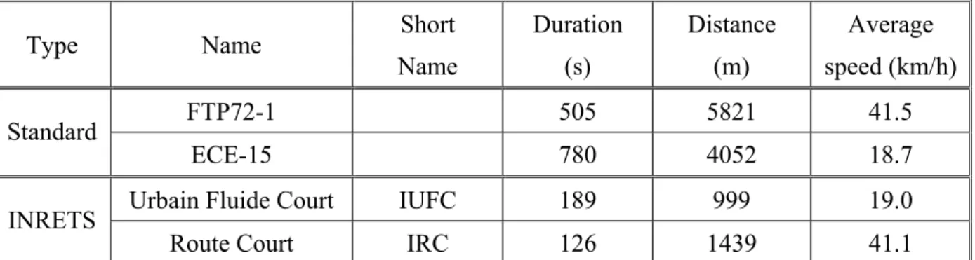
Type Name Short Name Duration (s) Distance (m) Average speed (km/h) FTP72-1 505 5821 41.5 Standard ECE-15 780 4052 18.7

Urbain Fluide Court IUFC 189 999 19.0

INRETS

Route Court IRC 126 1439 41.1

Table 1: Main characteristics of the various used cycles.

Cycle Name Emission Standard Fuel type CO CO2 FC HC NOx

EURO0 CAT. Gasoline 739 739 739 739

EURO0 W/O CAT. Gasoline 287 266 81 277 288

Diesel 3 3 3 3 EURO1

Gasoline 36 36 36 36

ECE15-1

EURO2 Gasoline 26 26 26 26

EURO0 CAT. Gasoline 727 727 10 727 727

Diesel 7 7 1 7 7 EURO0 W/O CAT.

Gasoline 16 16 16 16 16 Diesel 2 3 2 3 3 EURO1 Gasoline 3 3 3 3 3 Diesel 15 16 13 15 16 EURO2 Gasoline 5 5 5 5 5 Diesel 2 2 2 2 2 FTP72-1 EURO3 Gasoline 10 10 10 10 10

Diesel 2 3 2 3 3 EURO1 Gasoline 4 4 4 4 4 Diesel 13 16 9 17 17 EURO2 Gasoline 8 7 7 3 7 Diesel 3 4 4 4 4 IRC EURO3 Gasoline 11 12 6 10 12

Diesel 2 3 2 3 2 EURO1 Gasoline 2 4 4 2 4 Diesel 27 29 10 28 28 EURO2 Gasoline 10 16 16 12 13 Diesel 3 4 4 4 4 EURO3 Gasoline 43 45 27 41 42 IUFC EURO4 Gasoline 7 7 7 7 7

Table 2: Vehicle distribution versus average speed to calculate excess emission. To obtain the number of data, we have to multiply the number of vehicles by 2 for ECE15-1 and FTP72-1 cycle and by 15 for IUFC and IRC cycles.

(10)

For each vehicle, 2 types of cold and hot cycles were possibly followed (a short description of these cycles is shown in Table 1):

X Legislative cycles: ECE-15, FTP72-1.

X Inrets Short cycles: short free-flow urban (Inrets Urbain Fluide Court, so called IUFC) and short road (Inrets Route Court, so called IRC); each of these cycles was repeated 15 times. These cycles were drawn up from 23 000 travelled kilometres previously recorded all over France by 35 private cars (EUREV study, André, 1989; André, 1998; Joumard et coll., 1999).

Concerning excess emission data as a function of the cycle, the total number of obtained data was 29 825 (all categories and all pollutant merged). These data were measured with 1 556 vehicles. All samples were selected by various laboratories so that the distribution was representative, to some extent, of the fleet corresponding to each country. The number of vehicles tested by each laboratory and the corresponding cycles are shown in Table 2.

The annex 2 (Table 13, Table 14 and Table 15) detailed the Table 2 with the mean temperature of the measurements, the minimal and maximal temperature per cycle and per laboratory.

It should be noted that:

X for diesel cars with oxidation catalyst, the data are rare and do not allow a full data processing, as for other vehicle categories.

X for NOx pollutant, some laboratories made standard humidity correction but not all of them. We did not take into account such a correction factor and we think it would be better to have data without humidity corrections, i.e. actual emissions. Concerning these latter, Annex 6 gives the computation of the humidity correction factor.

(11)

1.2. Data correction

Once all the data were collected, we had to take into account a number of parameters influencing the general method:

X Great variety of data:

Ü as it can be seen in section 1.1, the number of vehicles analysed with standardised cycles is very significant; but such cycles are not representative since they do not reflect the reality. Comparing, for a same speed, the standard deviation of acceleration between Inrets and standard cycles [Joumard et al. (1995a)] yielded significantly differing results, acceleration standard deviation being lower than for standardised cycles.

Ü the representative cycles (real cycles) enabled a fine description of the emission evolution, but there was a limited number of analysed vehicles.

R In the Table 2, we can see that some categories have not enough vehicles to make a good computation of the cold start. So we decided to merge some categories. The consequences are that some results will be the same for different categories.

R When the vehicles are tested using a standard cycle, the engine temperature is not always hot at the end of the cycle, according to Joumard et al. (1995b). Therefore, we had to introduce a light adjustment for each pollutant. Thus we obtained excess emissions over the entire cold period for different cycles, whether standard or not. Such an adjustment is needed especially for ECE-15-1 cycle since it is very short. R Ambient temperature: it must be taken into account, if possible, whatever the mean

speed may be. Therefore, we have to look for a relation independent of the average speed, considering that initially the starts are made with a cold engine (engine temperature corresponds to ambient temperature at start).

R We make the following hypothesis: excess emission depends on the engine start temperature only (as temperature parameter), this one being equal to the ambient temperature (real cold start) or greater than the ambient temperature (semi-cold or semi-hot engine). This hypothesis is necessary due to the lack of data.

R Taking into account the travelled distance after a cold start in order to decrease excess emission levels if the travelled distance is lower than the cold distance (i.e. the distance needed to stabilise the emission).

It should be noted that some measurements correspond to the same cycle. But, they correspond to measurements made by various laboratories using various measuring devices, in various conditions, with various car models, different vehicle ages, etc.. So it results in differences for the same cycles themselves.

(12)

1.3. Cold start excess emission and distance calculation

1.3.1. Methods for regulated pollutants

We propose hereafter to analyse the different methods used to calculate the cold start emissions and the cold start distances, when emission factor is a continuous signal. It is the case when instantaneous emissions are available, but also when a short cycle is repeated as long as the emissions are stabilized.

1.3.1.1. First method: Standard deviation

This method was developed at INRETS (Joumard and Serié, 1999). It consists in the calculation of the standard deviation of the emission factors from the last emission factor to the first. If the emissions are in the hot part, the standard deviation is quite stable with a slight decrease, but when the cold emissions appear the standard deviation increases rapidly.

The cold start distance is determined when the standard deviation changes in its form.

The cold start emission is calculated by integrating the emissions until the cold start distance. Example:

The Figure 1 shows us the graphic representation of the emission of CO for Euro 1 Diesel at 18°C. On this figure we also plot the standard deviation. The standard deviation shows us that all the sub-cycles equal or higher than the sub-cycle 9 are hot. Thus the cold distance covers 8 sub cycles (i.e. 11.51 km). By integrating over the 8 first sub cycles we obtain the cold start emission of 0.89 g. 0 0,1 0,2 0,3 0,4 0,5 0,6 0,7 0,8 0,9 1 1 2 3 4 5 6 7 8 9 10 11 12 13 14 15 Sub-Cycle Number Emi s si o n F a ct o r (g ) 0 0,005 0,01 0,015 0,02 0,025 0,03 0,035 0,04 1 ,4 3 9 2 ,8 7 8 4 ,3 1 7 5 ,7 5 6 7 ,1 9 5 8 ,6 3 4 1 0 ,0 7 1 1 ,5 1 1 2 ,9 5 1 4 ,3 9 1 5 ,8 3 1 7 ,2 7 1 8 ,7 1 2 0 ,1 5 2 1 ,5 9 S ta n d a rd D e vi a ti o n (g )

CO EURO1 Diesel @ 18°C Standard Deviation

Cold Distance = 11.5 km

(13)

1.3.1.2. Second method: Linear regression

This method was developed at EMPA (Weilenmann, 2001). It consists in the calculation of the linear regression of the cumulative emission factor over the points in the hot emission. The value of the regression at distance 0 gives the cold start emission.

The cold/hot limit is calculated by plotting two lines which are parallel to the linear regression. They have the same slope but the constant for the first one is 95% of the cold start emission and the second one 105%.

The last time the cumulative emission enters between these two lines is the cold start distance. Example:

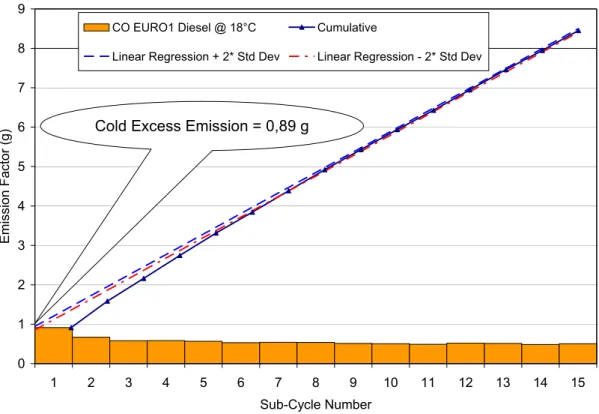
The Figure 2 and the Figure 3 show us the graphic representation of the emission of CO for Euro 1 Diesel at 18°C. On this figure we also plot the cumulative emission, the cold start emission (0.89 g) calculated from the linear regression (we took the last 7 points because the cumulative emissions curve is like a straight line) and the two lines at 95% and 105% of the cold start emission. Thus the cold distance is 6.2 sub cycles (i.e. 8.92 km).

This second method can give slightly different results, in term of cold distance and cold excess emission. The problem of this method is the determination of the hot sub-cycles, over which the hot linear regression is calculated.

0 1 2 3 4 5 6 7 8 9 1 2 3 4 5 6 7 8 9 10 11 12 13 14 15 Sub-Cycle Number Emi ssi o n F a ct o r (g )

CO EURO1 Diesel @ 18°C Cumulative

Linear Regression + 2* Std Dev Linear Regression - 2* Std Dev

Cold Excess Emission = 0,89 g

Figure 2: Example of cold start distance and emission calculation with the linear regression method.

(14)

3 3,2 3,4 3,6 3,8 4 4,2 4,4 4,6 4,8 5 4 5 6 7 8 Sub-Cycle Number E m is si o n F a ct o r (g ) Cumulative

Linear Regression + 2* Std Dev

Linear Regression - 2* Std Dev

Cold Distance = 8.92 km

Figure 3: Example of cold start distance and emission calculation with the linear regression method.

1.3.1.3. Artemis method: Linear Regression + Standard deviation

This method was developed during the Artemis project. We mixed the two above methods. We first plot the emission, the cumulative emission and the standard deviation (see Figure 4 and Figure 5).

The main calculation is based on the linear regression method. The cold start emission is the value of the linear regression at distance 0.

But, to calculate the cold start distance, we look at the intersection of two lines (± 2 standard deviations around the hot emissions) with the emission factors curve.

To obtain the hot emissions, we look at the standard deviation of the emissions as in the first method. We obtain the distance where the emissions are surely hot. We calculate the hot emissions by averaging the emissions over these sub-cycles. We calculate the standard deviation of the hot emissions to obtain the two lines. When the emission factors curve “enters” for the last time between these two lines, we obtain the cold start distance.

(15)

0 1 2 3 4 5 6 7 8 9 1 2 3 4 5 6 7 8 9 10 11 12 13 14 15 Sub-Cycle Number Em issi o n F a ct o r (g ) 0 1 2 3 4 5 6 7 8 9

CO EURO1 Diesel @ 18°C Hot Emission

Cumulative Linear Regression

Cold Emission = 0.90 g

Figure 4: Example of cold start distance and emission calculation with the Artemis method. The graphic cold start emission is obtained at the sub-cycle “-0.5”.

0 0,1 0,2 0,3 0,4 0,5 0,6 0,7 0,8 0,9 1 1 2 3 4 5 6 7 8 9 10 11 12 13 14 15 Sub-Cycle Number E m issi o n F a ct o r (g ) 0,000 0,005 0,010 0,015 0,020 0,025 0,030 0,035 0,040 0,045 0,050 St a n d a rd D e vi a ti o n (g ) CO EURO1 Diesel @ 18°C Standard Deviation Hot Emission Hot + 2* Std Dev Hot - 2* Std Dev Cold Distance = 10.3 km

(16)

1.3.1.4. Conclusion

The Table 3 shows us that the three methods give nearly the same cold start excess emission, but not the same cold start distance. The difference between cold distances goes up to 22 %.

Method Standard deviation Linear regression Artemis

Cold distance (km) 11.5 8.9 10.3

Cold emission (g) 0.89 0.89 0.90

Table 3: Comparison of the cold start distance and the cold start emission calculated with the different methods.

With the third method, we can determine:

X When the cycle is completely hot as in the first method

X The cold start emission as in the second method but with more accuracy because we applied the linear regression with the hot emissions

X The cold start distance with a better accuracy because we are searching when the hot emission cuts the emission by looking at the standard deviation of the hot part.

1.3.2. Methods for non regulated pollutants

The emissions factors of the non regulated pollutants for the cold start conditions were only available with the short Inrets cycles. The emissions were measured with two different conditions. At INRETS the non regulated pollutants emission factors were measured with a cold short cycle and with a hot one. So the cold start excess emission is the difference between this two values because the cold short cycle is always hot at the end.

The others laboratories measured the non regulated pollutants emission factors with the same cycle. They have 3 emissions factors per cycle (1 per 5 sub cycles). So to calculate the excess emission, we consider that the cold distance is equivalent for each non regulated pollutant and for the total HC. The cold distance of HC is always less than 10 sub cycles (cf. Table 6). With this condition, the excess emission is :

Excess Emission = EF(sub cycles 1 to 5) - EF(sub cycles 11 to 15) + EF(sub cycles 6 to 10) - EF(sub cycles 11 to 15)

(17)

1.3.3. Results

1.3.3.1. Categories merging for temperature and the speed influence

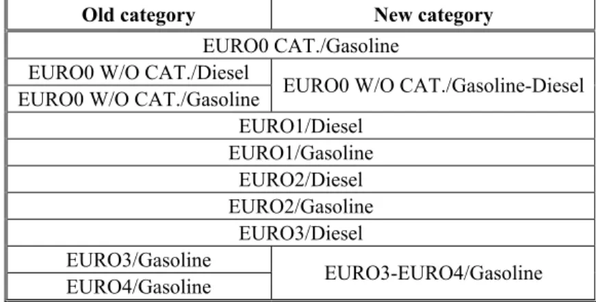
As we could see in the Table 2, some categories have not enough vehicles to make a quite good computation of the temperature and the speed influence. So we decided to merge some categories for these computations. The Table 4 gives the changes made.

Old category New category

EURO0 CAT./Gasoline EURO0 W/O CAT./Diesel

EURO0 W/O CAT./Gasoline EURO0 W/O CAT./Gasoline-Diesel

EURO1/Diesel EURO1/Gasoline EURO2/Diesel EURO2/Gasoline EURO3/Diesel EURO3/Gasoline EURO4/Gasoline EURO3-EURO4/Gasoline

Table 4: Categories merging to allow computations over a greater number of vehicles.

As you would see, this merging is not applied for the calculation of the cold distance and the cold start excess emission of the Inrets short cycles. It is better to have the absolute cold start excess emission and absolute cold start distance.

1.3.3.2. ECE-15 emissions correction

A previous study (Joumard et al., 1995b) showed that ECE-15 cycle could not cover entirely the cold period due to the cold start. So, we introduced a correction coefficient for this cycle to transform the measured excess emission during standard cycles into a full cold excess emission. This coefficient is deduced from measurement data recorded using IUFC cycle (because the mean speed is near the ECE-15 mean speed), which covers the whole cold period. Using this “cold” distance (see Table 6), calculated with the Artemis method, and the Inrets short cycles data, we calculate the correction coefficient to be applied to adjust the standardised cycles to the representative cycles.

For example (see Figure 6), the ECE-15 cycle corresponds to an average speed of 18.7 km/h and a distance of 4052 m. For CO pollutant, the cold distance (distance necessary to stabilise the emission level) is equal to 8.2 km for the representative cycle with the nearest average speed, i.e. 18.8 km/h (from Table 6). Regarding excess emission (normalised by the total excess emission) as a function of the distance, the ECE-15 cycle corresponds to 96 % of the total excess emission of the short free-flow urban cycle. Then the factor is equal to 1.04 (=1/0.96). We applied this method to all the pollutants and fuel consumption (see Table 5). The correction factors are sometimes important (from 0.74 to 4).

(18)

0% 10% 20% 30% 40% 50% 60% 70% 80% 90% 100% 0 1 2 3 4 5 6 7 8 9 Distance (km) D ime n s io n le s s Exce ss Em issi o n 0 10 20 30 40 50 60 70 80 90 100 E m issi o n F a c to r (g )

Short Inrets Cycle Emission Factor Short Inrets Cycle Excess Emission 96% Cold distance = 8.307 km Distance of the ECE15-1 cycle = 4.052 km

Figure 6: Cumulative dimensionless excess emission (ratio of absolute excess cold start emission to total absolute excess cold start emission) as a function of the distance (km) for short free-flow urban cycle. Correction calculation example of ECE-15 cycle for CO pollutant and gasoline cars without catalyst.

(19)

Old EU EM STD Fuel type

Mean

Temperature CO CO2 FC HC NOx

16 1 1,104 1,052 1 1

EURO0 CAT. Gasoline

17 1 1 1 1 1 -20 1,041 1,081 1 1,016 1,560 -7 1 1,044 1 1,016 1,041 10 1 0,971 1,009 1 1 18 1 1 0,742 1 1 EURO0 W/O CAT. Gasoline 21 0,810 0,812 1 1 1 18 1,242 1 1,116 1 4,002 Diesel 21 1 1,070 1 1,277 1 16 1 1,149 1,072 1 0,983 17 1 1 1 1 1 EURO1 Gasoline 20 1 1 1 0,978 1 -20 1,062 1,146 1 1,049 1,029 -7 1,083 1,123 1 1,098 1 22 1,074 1 1 1,118 -2,749 Diesel 23 1 1,111 1,081 1 1 -20 1,003 1,347 1,112 1,010 1 -8 1 1 1 1,006 1 21 1 1,198 1,142 1 1 23 1 1 1 0,983 1 EURO2 Gasoline 25 1 1 1 1 1 22 1 1,124 1,119 0,936 1 Diesel 23 0,937 1 1 1 1 -19 1 1,241 1 1,005 0,881 -18 1 1 1,194 1 1 -8 1,006 1,200 1,207 1,003 1 22 1 1,101 1,159 1 1 EURO3 Gasoline 23 1 1 1 0,999 1 -19 1,018 1,272 1,183 1,009 1 -8 1,029 1,156 1,102 1,006 0,768 EURO4 Gasoline 23 1,029 1 1 1 0,774

Table 5: Correction factor of cold excess emission for ECE-15 cycle, to take into account the too short distance of the cycles.

(20)

Cycle Emission Standard Fuel type

Mean

Temperature CO CO2 FC HC NOx

16 5,80 5,55 2,93 1,83

EURO0 CAT. Gasoline

17 2,69 -20 8,31 6,38 6,93 6,44 -7 2,88 4,85 5,43 8,97 10 3,96 5,19 5,19 1,26 3,41 18 6,96 EURO0 W/O CAT. Gasoline 21 6,31 7,21 2,23 0,58 18 8,74 6,82 8,23 Diesel 21 7,73 8,66 16 4,46 4,54 4,92 17 3,60 EURO1 Gasoline 20 5,97 -20 7,75 6,41 9,01 4,78 -7 6,63 7,32 9,56 2,86 22 5,85 8,04 9,87 Diesel 23 7,50 6,46 -20 7,22 9,13 9,13 9,13 0,50 -8 3,70 2,66 2,82 5,89 0,93 21 8,42 8,43 23 7,49 1,00 EURO2 Gasoline 25 1,83 22 7,14 7,12 6,36 2,41 Diesel 23 5,46 -19 1,71 8,59 9,84 9,08 -18 8,36 -8 4,14 9,02 9,42 9,70 0,90 22 9,87 9,57 EURO3 Gasoline 23 1,85 6,84 0,99 -19 8,70 8,62 8,62 9,81 1,24 -8 7,88 6,17 6,23 9,74 8,41 IUFC EURO4 Gasoline 23 5,46 1,98 2,00 7,05 6,42

EURO0 CAT. Gasoline 15 8,90 9,40 9,33 4,06 8,72

13 12,08 EURO0 W/O CAT. Gasoline 17 12,04 13,65 12,40 1,51 18 10,57 9,38 Diesel 21 14,11 13,25 12,06 EURO1 Gasoline 17 2,74 7,86 8,56 5,04 7,58 22 12,20 11,75 10,34 9,56 Diesel 23 10,20 19 3,75 7,70 7,69 7,14 EURO2 Gasoline 22 8,02 Diesel 22 9,53 5,72 5,71 5,36 3,67 21 7,69 IRC EURO3 Gasoline 22 2,86 10,85 9,34 1,40

Table 6: Distance (km) necessary to warm up the engine according to the pollutant and the mean cycle speed (km/h). FC: Fuel consumption.

(21)

Cycle Emission Standard Fuel type Mean Temperature CO CO2 FC HC NOx

16 135 74.1 7.99 1.00

EURO0 CAT. Gasoline

17 58.3

-20 296 391 72.4 1.95

-7 173 178 32.1 0.201

10 99.8 138 123 11.7 -0.154

18 50.0

EURO0 W/O CAT. Gasoline

21 54.8 52.1 11.8 -0.223 18 2.17 60.2 -0.113 Diesel 21 150 0.419 16 68.5 48.5 2.00 17 28.9 EURO1 Gasoline 20 8.52 -20 12.3 588 5.56 3.72 -7 6.53 411 1.38 2.07 22 2.85 0.431 -0.159 Diesel 23 147 42.9 -20 218 266 220 28.4 0.233 -8 85.6 166 105 9.96 0.819 21 139 56.4 23 3.97 0.848 EURO2 Gasoline 25 19.4 22 162 52.4 0.146 0.186 Diesel 23 2.09 -19 73.2 343 20.6 0.401 -18 107 -8 40.6 285 105 9.19 0.436 22 134 49.6 EURO3 Gasoline 23 8.49 1.45 0.486 -19 60.4 310 139 11.3 0.160 -8 52.4 180 90.4 7.75 0.123 IUFC EURO4 Gasoline 23 5.42 73.8 26.6 0.645 0.172 18 0.762 38.0 EURO1 21 109 0.201 -0.346 22 143 44.3 0.252 0.129 EURO2 23 1.72 Diesel EURO3 22 1.73 158 50.8 0.151 0.900 EURO0 CAT. 15 51.8 102 61.7 4.81 2.11 13 100

EURO0 W/O CAT.

17 95.0 135 10.1 -0.980 EURO1 17 29.9 79.3 43.6 4.42 1.69 19 16.4 147 55.0 1.20 EURO2 22 3.14 21 39.8 IRC Gasoline EURO3 22 9.65 173 1.96 0.687

Table 7: Cold start excess emission (g) according to the pollutant and the mean cycle speed (km/h). FC: Fuel consumption.

(22)

2. Influence of various parameters

In this chapter, the influence of the ambient temperature, average speed and distance on excess emissions will be shown. The aim is to express the excess emission as:

(

T V

δ

)

ω

f

( ) ( )

T V h

δ

EE , , = ₂₀_°_C_,₂₀_km_/_h⋅ , ⋅ (1) with:

EE (T, V, δ) is the excess emission T is the temperature

V is the average speed

δ=d/dc is the dimensionless distance (travelled distance d divided by the cold distance dc) ω20°C,20km/h is the excess emission at 20 °C and 20 km/h

f(T,V) = ω(T,V)/ ω20°C,20km/h is the cycle speed and the temperature influence dimensionless function expressed in section 2.1

h(δ) is the distance influence function expressed in section 2.2

2.1. Excess emission as a function of the cycle speed and the

temperature

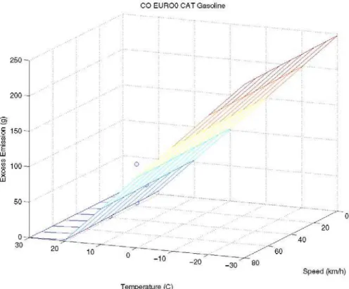
In Figure 7, an example of CO2 excess emission as a function of the mean speed for Euro 0 without catalyst gasoline vehicles is shown. The successive corrections are calculated and applied as follows:

X Merging the categories as explained in section 1.3.3.1.

X Data correction for ECE15-1 standard cycle, as explained in section 1.3.3.2.

Then, using modified data, we applied a 3D linear regression in order to obtain the excess emission level [g] as a function of the average speed V [km/h] and the temperature T [°C] (see Table 8 and figures in the annex 4).

It should be noticed that the regression is calculated using only four speed measurement points and different temperatures (the number of measurements points are indicated Table 8). One point in Figure 7 is the average of the excess emission for one temperature and one speed. But the regression was made by weighting each point by the number of vehicles. Using the calculated equations, we determined the correction coefficients (see Table 8) corresponding to the functions made dimensionless by dividing them by their values calculated at 20 km/h and 20°C. It should be noted that the boundaries of the measurements points for the linear regression calculation are [-20°C, +30°C] for the ambient temperature and [18 km/h, 42 km/h] for the mean speed. So outside these boundaries, the values of the

(23)

For all the data, fuel consumption was calculated using the carbon balance method. We used the formula (2) where the ratio hydrogen/carbon rH/C is equal to 1.8 for gasoline (leaded or unleaded) and 2.0 for diesel. The HC mass has to be expressed in CH4 equivalent.

011 . 12 mass Particle 043 . 16 mass HC 011 . 28 mass CO 011 . 44 mass CO r 1.008 12.011 mass Fuel ₂ + + + = ⋅ + HC (2) (Joumard et al., 1995b)

This equation indicates that the CO2 emission is not the only factor of the fuel consumption. Joumard et al. (1990) showed, for gasoline vehicles without catalyst, that the fuel conversion rates respectively into CO2, CO and HC equals on average 78 %, 19 % and 4 %, with little variations depending on average speed. Of course, for vehicles emitting much less regulated pollutants (as 3 way catalyst vehicles or diesel powered vehicles), CO2 rate is much higher.

Figure 7: Example of CO excess emission as a function of the mean speed and the temperature for Euro 0 without catalyst gasoline vehicles.

(24)

Pollutant Standard Emission Fuel Type

# of point

s

Excess Emission Equation

ω(T,V) Correction Coefficient f(T,V) MDC TDC VDC Typical Error EURO0 CAT. Gasoline 4 102,191 -4,865*T -0,042*V 25,227 -1,201*T -0,01*V 0,6827 0,4661 0,4653 4,2528

EURO0 W/O CAT. Gasoline/Diese l 9 67,17 -5,624*T + 2,462*V 17,155 -1,436*T + 0,629*V 0,8737 0,7633 0,7620 23,4155 Diesel 4 2,864 + 0,039*T -0,077*V 1,363 + 0,019*T -0,037*V 0,9615 0,9244 0,8992 0,2312 EURO1 Gasoline 4 28,149 + 0,72*T -0,47*V 0,849 + 0,022*T -0,014*V 0,8543 0,7298 0,7169 3,2999 Diesel 5 8,143 -0,202*T -0,077*V 3,172 -0,079*T -0,03*V 0,9587 0,9192 0,9161 1,0639 EURO2 Gasoline 6 13,112 -0,429*T + 0,174*V 1,636 -0,054*T + 0,022*V 0,1553 0,0241 -0,0193 34,2348 EURO3 Diesel 3 2,948 - 0,044*V 1,431 - 0,022*V 0,6350 0,4032 0,1370 0,6719 CO EURO3/EURO4 Gasoline 8 37,092 -1,46*T -0,054*V 5,448 -0,214*T -0,008*V 0,9749 0,9505 0,9490 6,0010 EURO0 CAT. Gasoline 4 198,07 -8,081*T -0,375*V 6,842 -0,279*T -0,013*V 0,6563 0,4308 0,4300 8,7143

EURO0 W/O CAT. Gasoline/Diese l 9 113,613 -6,83*T + 2,181*V 5,506 -0,331*T + 0,106*V 0,8542 0,7297 0,7280 30,5919 Diesel 4 194,797 + 1,709*T -4,099*V 1,325 + 0,012*T -0,028*V 0,7416 0,5499 0,4499 39,2526 EURO1 Gasoline 4 83,605 + 0,755*T -1,108*V 1,092 + 0,01*T -0,014*V 0,5061 0,2561 0,2223 12,2199 Diesel 5 405,016 -10,311*T -2,868*V 2,864 -0,073*T -0,02*V 0,9608 0,9232 0,9206 48,4942 EURO2 Gasoline 6 132,266 + 1,758*T -1,811*V 1,008 + 0,013*T -0,014*V 0,4183 0,1750 0,1420 47,6549 EURO3 Diesel 3 -113,973 + 16*T -2,295*V -0,712 + 0,1*T -0,014*V 0,4490 0,2016 -0,0265 59,3968 CO2 EURO3/EURO4 Gasoline 8 246,601 -5,026*T -1,016*V 1,961 -0,04*T -0,008*V 0,8934 0,7982 0,7925 47,5357

EURO0 CAT. Gasoline 3 8111,98 -280,486*T -127,594*V -163,437 + 5,651*T + 2,571*V 1 1 1 0

EURO0 W/O CAT. Gasoline/Diese l 7 70,624 -1,997*T + 0,133*V 2,119 -0,06*T + 0,004*V 0,6083 0,3700 0,3647 25,1778 Diesel 3 43,66 + 2,5*T -1,744*V 0,743 + 0,043*T -0,03*V 0,8155 0,6650 0,4416 18,3815 EURO1 Gasoline 3 -19,045 + 3,587*T -0,221*V -0,395 + 0,074*T -0,005*V 1 1 1 0 Diesel 3 701,177 -32*T -0,941*V 16,55 -0,755*T -0,022*V 0,5457 0,2978 0,2494 15,6896 EURO2 Gasoline 5 128,974 -2,824*T -0,913*V 2,378 -0,052*T -0,017*V 0,8546 0,7303 0,7078 22,1920 EURO3 Diesel 3 26,796 + 2*T -0,743*V 0,516 + 0,039*T -0,014*V 0,4574 0,2092 -0,0167 18,7913 FC EURO3/EURO4 Gasoline 8 104,887 -1,728*T -1,221*V 2,284 -0,038*T -0,027*V 0,9550 0,9120 0,9082 11,7696

(25)

Pollutant Standard Emission Fuel Type

# of point

s

Excess Emission Equation ωT,V

Correction Coefficient

f(T,V) MDC TDC VDC Typical Error

EURO0 CAT. Gasoline 4 9,177 -0,419*T -0,004*V 12,893 -0,589*T -0,006*V 0,5148 0,2650 0,2640 0,5705 EURO0 W/O CAT. Gasoline/Diese l 9 20,406 -1,244*T + 0,23*V 158,58 -9,666*T + 1,787*V 0,8627 0,7442 0,7428 5,2385 Diesel 4 0,502 + 0,009*T -0,014*V 1,235 + 0,022*T -0,034*V 0,9054 0,8198 0,7797 0,0697 EURO1 Gasoline 4 8,169 + 0,246*T -0,223*V 0,946 + 0,029*T -0,026*V 0,9900 0,9802 0,9792 0,2380 Diesel 5 2,321 -0,098*T -0,005*V 9,034 -0,382*T -0,02*V 0,8891 0,7905 0,7831 0,7509 EURO2 Gasoline 6 4,06 -0,004*T -0,06*V 1,461 -0,001*T -0,022*V 0,1267 0,0160 -0,0308 4,5144 EURO3 Diesel 3 0,551 -0,019*T -0,002*V 3,797 -0,128*T -0,012*V 0,3789 0,1436 -0,1011 0,0554 HC EURO3/EURO4 Gasoline 8 8,395 -0,393*T + 0,008*V 12,335 -0,578*T + 0,011*V 0,9350 0,8743 0,8708 2,6069 EURO0 CAT. Gasoline 4 4,076 -0,19*T -0,002*V 16,556 -0,771*T -0,007*V 0,9274 0,8600 0,8598 0,0625

EURO0 W/O CAT. Gasoline/Diese l 9 0,796 -0,029*T -0,016*V -7,683 + 0,278*T + 0,157*V 0,7482 0,5598 0,5573 0,2244 Diesel 4 0,52 -0,028*T -0,004*V -4,317 + 0,233*T + 0,033*V 0,9686 0,9382 0,9228 0,1224 EURO1 Gasoline 4 1,427 + 0,067*T -0,034*V 0,686 + 0,032*T -0,016*V 0,9736 0,9479 0,9455 0,1516 Diesel 5 1,363 -0,09*T + 0,013*V -7,335 + 0,484*T -0,067*V 0,9897 0,9796 0,9789 0,1777 EURO2 Gasoline 6 0,467 + 0,024*T -0,005*V 0,561 + 0,028*T -0,006*V 0,7151 0,5113 0,4905 0,3260 EURO3 Diesel 3 -0,565 + 0,02*T + 0,019*V -2,693 + 0,093*T + 0,092*V 0,5620 0,3159 0,1204 0,3681 NOx EURO3/EURO4 Gasoline 8 0,484 + 0,002*T -0,004*V 1,07 + 0,005*T -0,009*V 0,1857 0,0345 0,0061 0,2157

Table 8: Equation describing the influence of mean speed V [km/h] and ambient temperature T [°C] on excess emission

ω

(T,V)[g] and the associated dimensionless correction coefficients f(V,T). This equation results in a 3D linear regression (best fitted plan). These equations must be applied with the positive results. MDC=Multiple determination coefficient, TDC= Temperature determination coefficient, VDC = Speed determination coefficient.

(26)

2.2. Excess emission as a function of the travelled distance

The knowledge of the emission evolution during the cold phase, by considering the emissions measured on each Inrets short cycles, allows us to model the excess emission according to the travelled distance. The excess emission is therefore increasing till the end of the cold distance, and then equal to the cold start excess emission presented in section 2.1.

In a first step, we model the cold distance dc as a function of the vehicle speed V and the ambient temperature T by a 3D linear regression (see Table 9 and an example Figure 8; the others ones are in annex 5). Both excess emission and cold distance are therefore expressed as function of V and T.

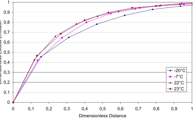
It allows us to make dimensionless both excess emission and travelled distance (see en example Figure 9; the others ones in annex 6) and to look at the influence of the dimensionless travelled distance δ=d/dc on the dimensionless excess emission. We express this influence as an exponential function h(δ). It should be noted that the chosen exponential function is well representative of the majority of the data. But in some cases, especially for NOx, the shape is much more complex (as shown in Annex 5.5). As we prefer to model only the influence of the distance, we propose to use the exponential function in all the cases.

This function h(δ) could be influenced by two available parameters, i.e. the ambient temperature T and the average speed V. But in fact the influence of V is very low and we consider only the influence of T. Therefore h(δ) can be expressed as:

( )

( ) ) ( 1 1 T a T a e e h − − = ⋅δ

δ

with c d d =

δ

(3)

where a(T) corresponds to the temperature dependence of dimensionless excess emission. a(T) is given in Table 10 for the different vehicle categories: we choose for a(T) a linear

regression.

(27)

Figure 8: Cold distance dc (km) as a function of the vehicle mean speed V (km/h) and the

ambient temperature T (°C) for CO2 pollutant on Euro 2 gasoline car.

Pollutant Standard Emission Fuel type # of

points dc (T,V) MDC TDC VDC Typical error

EURO0 CAT. Gasoline 2 24,146 -0,937*T -0,143*V 1 1 1 0

EURO0 W/O CAT. Gasoline/Diesel 5 -0,415 -0,016*T + 0,311*V 0,900 0,810 0,801 1,595

Diesel 2 4,666 + 0,125*T + 0,083*V 1 1 1 0 EURO1 Gasoline 2 7,312 -0,148*T -0,039*V 1 1 1 0 Diesel 4 2,84 -0,041*T + 0,199*V 0,994 0,989 0,988 0,204 EURO2 Gasoline 4 1,997 -0,099*T + 0,091*V 0,924 0,854 0,833 0,561 EURO3 Diesel 2 1,319 + 0,031*T + 0,185*V 1 1 1 0 CO EURO3/EURO4 Gasoline 7 2,784 -0,035*T + 0,019*V 0,306 0,093 0,062 1,808

EURO0 CAT. Gasoline 2 -2,8 + 0,192*T + 0,25*V 1 1 1 0

EURO0 W/O CAT. Gasoline/Diesel 5 -0,166 + 0,027*T + 0,323*V 0,982 0,964 0,962 0,729

Diesel 2 -9,013 + 0,563*T + 0,289*V 1 1 1 0 EURO1 Gasoline 2 0,917 + 0,031*T + 0,154*V 1 1 1 0 Diesel 4 3,098 + 0,021*T + 0,211*V 0,997 0,994 0,994 0,192 EURO2 Gasoline 4 7,019 + 0,09*T -0,027*V 0,611 0,373 0,307 1,396 EURO3 Diesel 2 17,427 -0,453*T -0,064*V 1 1 1 0 CO2 EURO3/EURO4 Gasoline 7 7,342 + 0,018*T + 0,077*V 0,503 0,253 0,228 1,482

EURO0 W/O CAT. Gasoline/Diesel 3 -2,535 + 0,178*T + 0,312*V 1 1 1 0

Diesel 2 -16,636 + 1,063*T + 0,116*V 1 1 1 0

EURO1

(28)

Pollutant Standard Emission Fuel type # of

points dc (T,V) MDC TDC VDC Typical error

EURO0 W/O CAT. Gasoline/Diesel 5 -5,393 -0,128*T + 0,495*V 0,988 0,977 0,976 0,719

Diesel 2 16,575 -0,594*T + 0,208*V 1 1 1 0 EURO1 Gasoline 2 6,775 + 0*T + -0,042*V 1 1 1 0 Diesel 4 6,791 -0,033*T + 0,102*V 0,973 0,948 0,945 0,236 EURO2 Gasoline 4 6,758 + 0,007*T + 0,027*V 0,365 0,133 -0,024 0,823 EURO3 Diesel 2 12,23 -0,25*T -0,046*V 1 1 1 0 HC EURO3/EURO4 Gasoline 7 6,468 -0,08*T + 0,109*V 0,983 0,966 0,965 0,251

EURO0 W/O CAT. Gasoline/Diesel 5 4,48 -0,18*T + 0,015*V 0,915 0,838 0,830 1,198

Diesel 2 1,497 + 0,172*T + 0,173*V 1 1 1 0 EURO1 Gasoline 2 2,622 + 0*T + 0,121*V 1 1 1 0 Diesel 4 6,588 + 0,16*T -0,006*V 0,937 0,878 0,872 0,959 EURO2 Gasoline 4 -4,424 + 0,007*T + 0,278*V 1 0,999 0,999 0,075 EURO3 Diesel 2 -4,291 + 0,281*T + 0,057*V 1 1 1 0 NOx EURO3/EURO4 Gasoline 7 3,286 -0,124*T + 0,014*V 0,625 0,390 0,369 2,742

Table 9: Formula describing the cold distance dc (km) as a function of the average speed V

(km/h) and the temperature T (°C). The results of this formula must be positive.

0 0,1 0,2 0,3 0,4 0,5 0,6 0,7 0,8 0,9 1 0 0,1 0,2 0,3 0,4 0,5 0,6 0,7 0,8 0,9 1 Dimensionless Distance D im e n s io n le s s Ex ce ss Emi ssi o n -20°C -7°C 22°C 23°C

Figure 9: Temperature influence on the dimensionless excess emission for Euro 2 diesel cars on CO2 pollutant, according to the dimensionless distance.

(29)

Pol. EU_emis_standard Fuel

type a(T) Pol. EU_emis_standard

Fuel

type a(T)

EURO0 CAT. Gasoline 3,0117*T -57,052 EURO0 CAT. Gasoline -0,5797*T + 3,104

EURO0 W/O CAT. Gasoline -0,138*T -7,166 EURO0 W/O CAT. Gasoline 0,0617*T -4,971 Diesel -3,535 Diesel -3,647 EURO1

Gasoline -6,487 EURO1 Gasoline -1,6153*T + 22,951

Diesel 0,013*T -4,769 Diesel 0,0365*T -5,367

EURO2

Gasoline 0,0708*T -7,066 EURO2 Gasoline -0,1755*T -10,790

Diesel 4,942*T -123,364 Diesel -5,619

EURO3

Gasoline -0,0105*T -5,719 EURO3 Gasoline -0,0765*T -10,936

CO

EURO4 Gasoline 0,0453*T -6,115

HC

EURO4 Gasoline -0,2763*T -14,426

EURO0 CAT. Gasoline 0,1929*T -6,629 EURO0 CAT. Gasoline 0,8063*T -15,710

EURO0 W/O CAT. Gasoline -0,0261*T -4,351 EURO0 W/O CAT. Gasoline -0,1459*T -5,324 Diesel -5,131 Diesel -0,4953*T + 7,777 EURO1

Gasoline -0,7775*T + 10,367 EURO1 Gasoline -1,3613*T + 13,946

Diesel -0,0188*T -3,926 Diesel 0,0837*T -3,029

EURO2

Gasoline -0,0182*T -2,658 EURO2 Gasoline 0,1006*T -4,617

Diesel -3,208 Diesel -2,626

EURO3

Gasoline -0,0217*T -4,228 EURO3 Gasoline 0,8659*T -16,396

CO2

EURO4 Gasoline 0,0396*T -2,583

NOx

EURO4 Gasoline -0,4427*T -60,590

EURO0 CAT. Gasoline 0,312*T -9,427

EURO0 W/O CAT. Gasoline -0,2066*T -3,223 Diesel -3,601 EURO1 Gasoline -0,7282*T + 8,510 Diesel -0,0924*T -2,075 EURO2 Gasoline 0,0092*T -3,516 Diesel -3,236 EURO3 Gasoline 0,0033*T -3,870 FC EURO4 Gasoline 0,0484*T -2,986

Table 10: Equation describing the temperature influence on the dimensionless excess emission as a function of the dimensionless distance

δ

(

δ

=d/dc).

(30)

2.3. General formula of cold-start-related excess emissions of a

trip

We assumed that the general model of the cold start emission is a function of ambient temperature, average speed and travelled distance. Measurements were made using different cycles, these being characterised by their mean speed (see Table 1). The cycles can be characterised by other parameters such as mean product speed times acceleration (dynamics measurement), standard deviation of speed or standard deviation of the product speed times acceleration for example (Hassel and Weber, 1996). But, those parameters can not be used in the general model due to the fact that there is no available statistics.

With the calculation made in section 2, the equation (1) can be written as:

(

)

( )

      − − ⋅ ⋅ = ° ( ) ) ( / 20 , 20 1 1 , , , _a_T T a h km C e e V T f V T EE δ ω δ where:

EE: Excess emission for a trip in g

V: mean speed in km/h during the cold period

T: temperature in °C (ambient temperature for cold start, engine start temperature for starts at an intermediate temperature)

( )

T V

d d

c ,

=

δ

the dimensionless distance with d: the travelled distance

dc: the cold distance

ω20°C,20km/h: reference excess emission (at 20 °C and 20 km/h).

The function ω20°C,20km/h, f(T,V), a(T), dc(T,V) can be found respectively in Table 11, Table 8, Table 10 and Table 9. The function f must be positive or null.

(31)

Pollutant Emission Standard Fuel type ω20°C,20km/h

(g) Pollutant Emission Standard Fuel type

ω20°C,20km/h (g)

EURO0 CAT. Gasoline 4,051 EURO0 CAT. Gasoline 0,712

EURO0 W/O CAT. Gasoline/Diese

l 3,916 EURO0 W/O CAT.

Gasoline/Diese

l 0,129

Diesel 2,102 Diesel 0,407

EURO1

Gasoline 33,149 EURO1 Gasoline 8,640

Diesel 2,567 Diesel 0,257

EURO2

EURO3 Diesel 2,059 EURO3 Diesel 0,145

CO

EURO3/EURO4 Gasoline 6,809

HC

EURO0 CAT. Gasoline 28,950 EURO0 CAT. Gasoline 0,246

l 20,636 EURO0 W/O CAT.

Gasoline/Diese

l -0,104

Diesel 147,015 Diesel -0,121

EURO1

Diesel 141,435 Diesel -0,186

EURO2

EURO3 Diesel 160,132 EURO3 Diesel 0,210

CO2

EURO3/EURO4 Gasoline 125,769 NOx

EURO0 CAT. Gasoline -49,634

l 33,335 Diesel 58,785 EURO1 Gasoline 48,267 Diesel 42,367 EURO2 Gasoline 54,233 EURO3 Diesel 51,932 FC EURO3/EURO4 Gasoline 45,926

Table 11: Coefficient

ω

20°C,20km/h corresponding to excess emission at 20 °C and 20 km/h (in

g), calculated from Table 8.

For example, for CO pollutant and Euro 2 gasoline cars:

X Using Table 11, ω20°C,20km/h=8.012

X Using Table 8, f(T,V)= 1.008+0.013*T-0.014*V

X Using Table 10, a(T)=0.071*T-7.066

X Using Table 9, dc(T,V)= 1.997-0.099*T-0.091*V and therefore δ et h(δ) can be calculated, and finally:

(

)

( ) ( ) ( ) ( 4) 44443 4 4 4 4 4 2 1 4 4 4 4 3 4 4 4 4 2 1 3 2 1 V T d h T V T d T V T f e e V T , , 066 . 7 071 . 0 091 . 0 099 . 0 997 . 1 066 . 7 071 . 0 , Gasoline 2, Euro CO, 1 1 014 . 0 013 . 0 008 . 1 8.012 = V, T, Emission Excess           − − ⋅         ⋅ − ⋅ + ⋅ _⋅ ₊+ ⋅ − ⋅ + ⋅ ω

δ

(32)

joint influence of speed and temperature is ranging from 0 to 71, with an average of 11.5. Thus the influence of temperature and speed is very significant, temperature influence being higher than speed influence except for NOx, pollutant where speed influence being higher than temperature influence.

The light duty vehicles (LDV) are not concerned by our data base. Therefore we could consider, if necessary, that LDV excess emissions should be the same as for passenger cars (PC) but it would be much better to build a LDV cold start model using LDV specific data base.

Pollutant Standard Emission Fuel Type f(-10°C.20km/h) f(20°C.20km/h) f(20°C.50km/h) ) 50 , 20 ( ) 20 , 10 ( f f −

EURO0 CAT. Gasoline 37.0 1 0.7 53.8

EURO0 W/O CAT. Gasoline/Diesel 44.1 1 19.9 2.2

Diesel 0.5 1 0 - EURO1 Gasoline 0.4 1 0.6 0.6 Diesel 3.4 1 0.1 32.9 EURO2 Gasoline 2.6 1 1.7 1.6 EURO3 Diesel 1 1 0.4 2.8 CO EURO3/EURO4 Gasoline 7.4 1 0.8 9.7

Diesel 0.7 1 0.2 4.0 EURO1 Gasoline 0.7 1 0. 6 1.2 Diesel 3.2 1 0.4 8.1 EURO2 Gasoline 0.6 1 0. 6 1.0 EURO3 Diesel 0 1 0.6 0 CO2 EURO3/EURO4 Gasoline 2.2 1 0. 8 2.9

EURO0 CAT. Gasoline 0 1 78.1 0

Diesel 0 1 0.1 0 EURO1 Gasoline 0 1 0.9 0 Diesel 23.7 1 0.3 70.8 EURO2 Gasoline 2.6 1 0. 5 5.2 EURO3 Diesel 0 1 0.6 0 FC EURO3/EURO4 Gasoline 2.1 1 0.2 10.5

EURO0 W/O CAT. Gasoline/Diesel 291 1 54.6 5.3

Diesel 0.3 1 0 - EURO1 Gasoline 0.1 1 0.2 0.6 Diesel 12.5 1 0.4 31.1 EURO2 Gasoline 1.1 1 0.4 3.0 EURO3 Diesel 4.8 1 0.6 7.6 HC EURO3/EURO4 Gasoline 18.3 1 1.3 13.7

EURO0 W/O CAT. Gasoline/Diesel 0 1 5.7 0

Diesel 0 1 2.0 0 EURO1 Gasoline 0.1 1 0.5 0.1 Diesel 0 1 0 - EURO2 Gasoline 0.2 1 0.8 0.2 EURO3 Diesel 0 1 3.8 0 NOx EURO3/EURO4 Gasoline 0.8 1 0.7 1.1

Table 12: Influence of temperature and speed on the speed and temperature function f(T,V): comparison of 3 cases.

(33)

3. Conclusion

This modelling of excess emission under cold start conditions for passenger cars results from data provided by various European research organisations as part of MEET and Artemis

projects. The present model takes into account mean speed, ambient temperature and travelled distance. This model results from measurements made over 4 driving cycles. Average speeds of these cycles range from 18.7 km/h to 41.5 km/h and temperature measurements range from -20 °C to 28 °C.

The cold excess emission is obtained in grams and is valid for gasoline and diesel cars, from Euro 0 to Euro 4 emission standard. This emission is given for a prescribed pollutant and vehicle technology. The general formula is written in the form of a reference excess emission multiplied by functions depending on average speed, engine temperature and travelled distance. For fuel consumption, it was determined using the carbon balance method. The forms of speed-temperature functions were assumed to be 3D-linear. For travelled distance, we assumed that its influence was in the shape of an exponential function (with a temperature influence) for all pollutants in order to simplify the model, even if the shape seems more complicated for NOx pollutant. We also assumed that the trips were started with a cold engine, i.e. start engine temperature corresponding to ambient temperature. For intermediate start temperature conditions, we made the hypothesis that the excess emission corresponds to the cold start emission with the same start temperature: e.g. a start at an engine temperature of 30 °C corresponds to a cold start at an ambient temperature of 30 °C.

This model can be applied at different geographic scales: at a macroscopic scale (national inventories) using road traffic indicators and temperature statistics, or at a microscopic scale for a vehicle and a trip. If a model user could not access to necessary statistics, it would be recommended to integrate the statistics recorded at national level into the model, in order to further the model use and obtain a national average excess emission directly.

This study corresponds to the state-of-the-art at the present time. In the future, this model could be improved by different ways:

- updating this model using new data when available, either for the most recent passenger cars, or the light duty vehicles, or the heavy duty vehicles.

- it would be much more precise to have crossed distributions for different speeds and ambient temperatures.

- the number of analysed data has to be increased, especially for different speeds and low or high temperatures.

- intermediate engine temperatures must be considered, i.e. when engine start temperature does not correspond to ambient temperature (“ cool starts ”). It would be interesting to model start engine temperature as a function of ambient temperature, parking duration and maybe introduce an engine cooling coefficient.

(34)

Annex 1:

Laboratory acronyms, addresses and persons

to contact

Lab name Signification Contact

person Address

E-Mail (or phone and fax number) EMPA Eidgenössische Materialprüfungs- und Forschungsanstalt M. Weilenman n Überlandstrasse 129,

8600 Dübendorf, Switzerland martin.weilenmann@empa.ch

IM CNR Istituto Motori

National Research Council M. Rapone

viale Marconi 8

80125 Napoli, Italy mrap@motori.im.na.cnr.it

INFRAS AG

Infrastruktur-, Umwelt- und

Wirtschaftsberatung M. Keller

Mühlemattstrasse 45 CH-3007 Bern

Switzerland

mario.keller@infras.ch

INRETS _{sur les Transports et leur Sécurité}Institut National de Recherche R. Joumard

Case 24 F-69675 Bron Cedex

France

joumard@inrets.fr

INTA Instituto Nacional de Tecnica

Aeroespacial J. P. Laguna Ctra de Ajalvir km 4 28850 Torrejón de Ardoz (Madrid) Spain +34-15201723 +34-15201319

KTI Institute for Transport Sciences T. Mereteï

XI. Thán Károly u. 3-5 1119 Budapest

Hungary

meretei@mercury.kti.hu

LAT Lab. Applied Thermodynamics Z. Samaras

Aristotle Univ. Thessaloniki 54006 Thessaloniki Greece zisis@auth.gr Politecnico di Milano S. Cernushi P.za L. da Vinci, 32 I-20133 Milano Italy +39-223996411 +39-223996499

TNO Netherlands org. for applied

scientific research R. Vermeulen P.O. Box 6033 2600 JA Delft The Netherlands vermeulen@wt.tno.nl

TRL Transport Research Laboratory I. MacCrae

Old Wokingham road Crowthorne Berkshire RG

45 6AU England

imccrae@trl.co.uk

TU-Graz Graz University of Technology S.

Hausberger Kopernikusgasse 24 A-8010 Graz Austria hausberger@vkmb.tu-graz.ac.at

TÜV TÜV Rheinland Sicherheit und

Umweltschutz GmbH D. Hassel

Konstantin Wille Strasse 1 D-51105 Köln

Germany

+49-2218062479

+49-2218061756

VTI _{Transport Research Institute}Swedish National Road and

U. Hammarstr öm Statens väg- och transportforskninginstitut S-581 95 Linköping Sweden ulf.hammarstrom@vti.se

(35)

Annex 2:

Vehicles, data and temperature distribution

The next tables give the number of vehicles by pollutant, by laboratory, by category at the mean temperature of the vehicles measurements.

Cycle Name Emission Standard Fuel type Mean Temperature CO CO2 FC HC NOx

11 36 33 35 34 35

19 46

20 251 233 243 253 Diesel -7 3 3 3 3 EURO1 Gasoline -7 36 36 36 36 ECE15-1 EURO2 Gasoline -7 26 26 26 26 15 10

EURO0 CAT. Gasoline

20 727 727 727 727

19 7 Diesel

20 7 1 7 7

EURO0 W/O CAT.

Gasoline 17 16 16 16 16 16 19 2 Diesel 20 3 2 3 3 15 3 EURO1 Gasoline 20 3 3 3 3 20 13 Diesel 21 15 16 15 16 EURO2 Gasoline 16 5 5 5 5 5 20 2 Diesel 21 2 2 2 2 FTP72-1 EURO3 Gasoline 22 10 10 10 10 10

EURO0 CAT. Gasoline 16 10 10 10 10 10

11 8 8 8 8

13 10

21 9 9 9

22 8 21 2 Diesel 22 2 3 3 3 EURO1 Gasoline 16 4 4 4 4 4 21 9 Diesel 22 13 16 17 17 19 8 7 7 7 EURO2 Gasoline 22 3 21 4 Diesel 22 3 4 4 4 21 6 IRC EURO3 Gasoline 22 11 12 10 12

(36)

Cycle Name Emission Standard Fuel type Mean Temperature CO CO2 FC HC NOx

16 10 8 10

EURO0 CAT. Gasoline

17 9 9

-20 6 6 6 6

-7 6 6 6 6

12 10 10 10 10

13 11

23 7 7 7 7 22 2 3 2 3 2 Diesel 16 4 4 4 EURO1 Gasoline 17 2 2 -20 6 6 6 6 -7 6 6 6 6 Diesel 22 15 17 10 16 16 -12 3 3 3 3 3 21 12 12 23 8 9 EURO2 Gasoline 25 6 Diesel 22 3 4 4 4 4 -19 12 12 12 12 -18 6 -8 11 11 6 11 11 21 20 22 EURO3 Gasoline 22 15 18 19 -19 2 2 2 2 -18 2 -8 3 3 3 3 3 21 2 2 IUFC EURO4 Gasoline 22 2 2 2

Table 13: Number of vehicles by cycle (defined in section 1.1), by pollutant, by category at the mean temperature of the vehicles measurements.

(37)

Cycle Name Old EU EM STD Fuel type Mean Temperature EMPA INRETS IM TNO VTT

EURO0 CAT. Gasoline 20 2956

13 220

20 117 772

21 26

14 64 Diesel -7 12 EURO1 Gasoline -7 144 ECE15-1 EURO2 Gasoline -7 104 15 10

EURO0 CAT. Gasoline

20 40 2868

19 4 24

Diesel

14 1

EURO0 W/O CAT.

Gasoline 17 30 50 20 4 Diesel 22 9 EURO1 Gasoline 14 15 21 23 37 Diesel 22 6 9 EURO2 Gasoline 16 25 Diesel 17 10 FTP72-1 EURO3 Gasoline 22 30 20

EURO0 CAT. Gasoline 15 50

13 9 1

17 24 39 4 21 9 Diesel 18 4 EURO1 Gasoline 17 15 5 22 18 37 4 Diesel 23 6 6 1 19 21 8 EURO2 Gasoline 22 1 2 Diesel 22 9 10 21 4 2 IRC EURO3 Gasoline 22 24 13 8

(38)

Cycle Name Old EU EM STD Fuel type Mean Temperature EMPA INRETS IM TNO VTT

16 37

EURO0 CAT. Gasoline

17 9

-20 24 -7 24

21 24 12 4

18 3 1

10 35 21 6 Diesel 18 6 16 9 3 17 1 1 EURO1 Gasoline 20 1 1 -20 24 -7 24 22 18 26 3 Diesel 23 6 19 2 -20 5 -8 10 21 12 8 4 23 5 8 4 EURO2 Gasoline 25 4 2 22 8 8 Diesel 23 1 2 -19 24 24 -18 6 -8 24 30 22 6 8 10 12 EURO3 Gasoline 23 18 3 15 18 -19 10 -8 15 IUFC EURO4 Gasoline 23 10

Table 14: Number of vehicles per cycle (defined in section 1.1), per laboratory, per category at the mean temperature of the vehicles measurements.

(39)

Laboratory Cycle Name Temperature CO CO2 FC HC NOx Min 21,9 21,9 21,9 22,5 21,9 FTP72-1 Max 23,4 23,4 23,4 23,4 23,4 Min 23,0 23,0 23,0 23,0 IRC Max 23,0 23,0 23,0 23,0 Min -20,0 -20,0 -20,0 -20,0 EMPA IUFC Max 23,0 23,0 23,0 23,0 Min 8,0 8,0 8,0 8,0 8,0 ECE15-1 Max 27,0 27,0 27,0 27,0 27,0 Min 9,0 9,0 9,0 9,0 9,0 FTP72-1 Max 26,0 26,0 26,0 26,0 26,0 Min 6,0 6,0 6,0 6,0 6,0 IRC Max 25,0 28,0 25,0 28,0 28,0 Min 4,0 4,0 4,0 4,0 4,0 INRETS IUFC Max 27,0 28,0 28,0 27,0 27,0 Min 23,0 23,0 23,0 23,0 23,0 IRC Max 25,0 25,0 25,0 25,0 25,0 Min 23,5 23,5 23,5 23,5 23,5 ISTITUTO MOTORI IUFC Max 26,0 26,0 26,0 26,0 26,0 ECE15-1 Min 20,0 20,0 20,0 20,0 Max 20,0 20,0 20,0 20,0 FTP72-1 Min 20,0 20,0 20,0 20,0 TNO Max 20,0 20,0 20,0 20,0 ECE15-1 Min -7,0 -7,0 -7,0 -7,0 Max -7,0 -7,0 -7,0 -7,0 IUFC Min -20,0 -20,0 -20,0 -20,0 -20,0 VTT Max 23,7 23,7 23,7 23,7 23,7

Table 15: Minimal and maximal temperatures of the vehicles measurements per laboratory, per cycle (defined in section 1.1), per pollutant.

(40)

Annex 3:

Example of dimensionless excess emissions

versus distance (km)

The figure below shows the cumulative dimensionless excess emission (ratio of absolute excess cold start emission to total absolute excess cold start emission) as a function of the distance (km) for short Inrets free-flow urban cycle (IUFC).

This graphic explains why sometimes the correction factor can be less than 1.

0% 10% 20% 30% 40% 50% 60% 70% 80% 90% 100% 110% 120% 130% 140% 150% 160% 0 1 2 3 4 5 6 7 8 9 10 Distance (km) D im e n s io n le ss Ex ce ss Em is si o n 0 0,1 0,2 0,3 0,4 0,5 0,6 0,7 0,8 Emi s si o n F a ct o r (g ) Emission Factor Excess Emission 113%

Correction calculation example of ECE-15 cycle for NOx pollutant on EURO3 Gasoline cars (at -19°C).

(41)

Annex 4:

Excess emissions (g) versus vehicle speed

(km/h) and ambient temperature (°C)

A point represents an average of the data for the category, the speed and the temperature, and the plan is the regression curve (linear regression) associated to those data.

(42)

(43)

(44)

(45)

(46)

(47)

(48)

(49)

(50)

(51)

(52)

(53)

(54)

(55)

(56)

Annex 5:

Cold distance (km) as function of the vehicle

speed (km/h) and the temperature (°C).

(57)

(58)

(59)

(60)

(61)

(62)

(63)

(64)

(65)

(66)

(67)

(68)

(69)

(70)

(71)

Annex 6:

Dimensionless excess emission versus

dimensionless distance

In the figures, one point is for a given dimensionless distance the dimensionless excess emission averaged over 2 cycle speeds (see section 1.1.).

Annex 6.1:

CO

Euro 0 Cat. Gasoline 0 0,2 0,4 0,6 0,8 1 0 0,1 0,2 0,3 0,4 0,5 0,6 0,7 0,8 0,9 1 Dimensionless Distance D ime n si o n le s s Exce ss Emi ssi o n 15°C 17°C Euro 0 W/O Cat. Gasoline and diesel 0,2 0,4 0,6 0,8 1 1,2 1,4 D ime n s io n le ss Ex ce ss Emi ssi o n -20°C -7°C 10°C 17°C

(72)

Euro 1 diesel 0 0,1 0,2 0,3 0,4 0,5 0,6 0,7 0,8 0,9 1 0 0,1 0,2 0,3 0,4 0,5 0,6 0,7 0,8 0,9 1 Dimensionless Distance D ime n si o n le ss Exc e s s Emi s si o n 18°C 18°C Euro 1 Gasoline 0 0,2 0,4 0,6 0,8 1 1,2 0 0,1 0,2 0,3 0,4 0,5 0,6 0,7 0,8 0,9 1 Dimensionless Distance D ime n s io n le ss Ex ce ss Emi ssi o n 17°C 17°C Euro 2 Diesel 0,1 0,2 0,3 0,4 0,5 0,6 0,7 0,8 0,9 1 D ime n si o n le s s Exce ss Emi ssi o n -20°C -7°C 22°C

(73)

Euro 2 Gasoline 0 0,1 0,2 0,3 0,4 0,5 0,6 0,7 0,8 0,9 1 0 0,1 0,2 0,3 0,4 0,5 0,6 0,7 0,8 0,9 1 Dimensionless Distance D ime n si o n le ss Exc e s s Emi s si o n -20°C -8°C 19°C 25°C Euro 3 Diesel 0 0,2 0,4 0,6 0,8 1 1,2 0 0,1 0,2 0,3 0,4 0,5 0,6 0,7 0,8 0,9 1 Dimensionless Distance D ime n s io n le ss Ex ce ss Emi ssi o n 22°C 23°C Euro 3 Gasoline 0,2 0,3 0,4 0,5 0,6 0,7 0,8 0,9 1 D ime n s io n le ss Ex ce ss Emi ssi o n -19°C -8°C

(74)

Euro 4 Gasoline 0 0,1 0,2 0,3 0,4 0,5 0,6 0,7 0,8 0,9 1 0 0,1 0,2 0,3 0,4 0,5 0,6 0,7 0,8 0,9 1 Dimensionless Distance D ime n si o n le ss Exc e s s Emi s si o n -19°C -8°C 23°C

(75)

Annex 6.2:

CO2

Euro 0 Cat. Gasoline 0 0,1 0,2 0,3 0,4 0,5 0,6 0,7 0,8 0,9 1 0 0,1 0,2 0,3 0,4 0,5 0,6 0,7 0,8 0,9 1 Dimensionless Distance D ime n si o n le ss Exc e s s Emi s si o n 15°C 16°C Euro 0 W/O Cat. Gasoline and diesel 0 0,2 0,4 0,6 0,8 1 1,2 0 0,1 0,2 0,3 0,4 0,5 0,6 0,7 0,8 0,9 1 Dimensionless Distance D ime n s io n le ss Ex ce ss Emi ssi o n -20°C -7°C 10°C 17°C 21°C

(76)

Euro 1 diesel 0 0,1 0,2 0,3 0,4 0,5 0,6 0,7 0,8 0,9 1 0 0,1 0,2 0,3 0,4 0,5 0,6 0,7 0,8 0,9 1 Dimensionless Distance D ime n si o n le ss Exc e s s Emi s si o n 21°C 21°C Euro 1 Gasoline 0 0,1 0,2 0,3 0,4 0,5 0,6 0,7 0,8 0,9 1 0 0,1 0,2 0,3 0,4 0,5 0,6 0,7 0,8 0,9 1 Dimensionless Distance D ime n s io n le ss Ex ce ss Emi ssi o n 16°C 17°C Euro 2 Diesel 0,2 0,3 0,4 0,5 0,6 0,7 0,8 0,9 1 D ime n s io n le ss Ex ce ss Emi s s io n -20°C -7°C 22°C 23°C

(77)

Euro 2 Gasoline 0 0,1 0,2 0,3 0,4 0,5 0,6 0,7 0,8 0,9 1 0 0,1 0,2 0,3 0,4 0,5 0,6 0,7 0,8 0,9 1 Dimensionless Distance D im e n s io n le s s E x c e s s Em is s io n -20°C -8°C 19°C 21°C Euro 3 Diesel 0 0,1 0,2 0,3 0,4 0,5 0,6 0,7 0,8 0,9 1 0 0,1 0,2 0,3 0,4 0,5 0,6 0,7 0,8 0,9 1 Dimensionless Distance D ime n s io n le ss Ex ce ss Emi ssi o n 22°C 22°C Euro 3 Gasoline 0,2 0,3 0,4 0,5 0,6 0,7 0,8 0,9 1 D ime n s io n le ss Ex ce ss Emi ssi o n -19°C -8°C 22°C