Subauroral electron temperature enhancement in the nighttime ionosphere

(1)

HAL Id: hal-00318123

https://hal.archives-ouvertes.fr/hal-00318123

Submitted on 9 Aug 2006

HAL is a multi-disciplinary open access

archive for the deposit and dissemination of

sci-entific research documents, whether they are

pub-lished or not. The documents may come from

teaching and research institutions in France or

abroad, or from public or private research centers.

L’archive ouverte pluridisciplinaire HAL, est

destinée au dépôt et à la diffusion de documents

scientifiques de niveau recherche, publiés ou non,

émanant des établissements d’enseignement et de

recherche français ou étrangers, des laboratoires

publics ou privés.

Subauroral electron temperature enhancement in the

nighttime ionosphere

G. W. Prölss

To cite this version:

G. W. Prölss. Subauroral electron temperature enhancement in the nighttime ionosphere. Annales

Geophysicae, European Geosciences Union, 2006, 24 (7), pp.1871-1885. �hal-00318123�

(2)

Ann. Geophys., 24, 1871–1885, 2006 www.ann-geophys.net/24/1871/2006/ © European Geosciences Union 2006

Annales

Geophysicae

Subauroral electron temperature enhancement in the nighttime

ionosphere

G. W. Pr¨olss

Argelander Institut für Astronomie, Universität Bonn, Auf dem Hügel 71, 53121 Bonn, Germany Received: 16 March 2006 – Revised: 31 May 2006 – Accepted: 8 June 2006 – Published: 9 August 2006

Abstract. In the nightside subauroral region, heat transfer

from the ring current causes a significant increase in the elec-tron temperature of the upper ionosphere. Using DE-2 satel-lite data, we investigate the properties of this remarkable fea-ture. We find that the location of the temperature enhance-ment is primarily dependent on the level of geomagnetic ac-tivity. For geomagnetically quiet conditions (Dst '0), the temperature peak is located slightly poleward of 60◦

invari-ant latitude. For each decrease in the Dst index by 10 nT, it moves equatorward by about one degree. To a lesser degree, the location of the heating effect also depends on magnetic local time, with a significant positional asymmetry about midnight. The magnitude of the temperature enhancement varies with altitude. Within the height range 280 to 940 km, the peak temperature increases by 73%, on average. Thereby a conspicuous increase in the temperature gradient is ob-served above about 700 km altitude. The magnitude of the heating effect also depends on the level of geomagnetic activ-ity. For a decrease in the Dst index by 100 nT, the peak tem-perature increases by 46%, on average. This rate of increase, however, depends on season and is significantly smaller dur-ing winter conditions. A superposed epoch type of averag-ing procedure is used to obtain mean latitudinal profiles of the temperature enhancement. For an altitude of 500 km, the following mean properties are derived: amplitude '1100 K; width at half this peak value '2.7 deg; distance between equatorward boundary and maximum '3.6 deg. On average, a decrease in the electron density is observed at the location of the temperature enhancement, at least at 500 km altitude. At the same time, a moderate increase in the zonal ion drift speed is recorded at this location. During larger geomagnetic storms, the latitudinal profile of the temperature enhance-ment assumes a more step-function-like shape, with a broad increase in electron temperature poleward from the equato-rial edge of the electron temperature enhancement. Also the heating effects may extend to very low latitudes (less than 35◦_{invariant latitude). And residual heating effects are}

ob-Correspondence to: G. W. Pr¨olss ([email protected])

served long after the storm-substorm activity has ceased. The results obtained in this study should prove useful for both empirical and theoretical modeling of the nightside subauro-ral ionosphere.

Keywords. Ionosphere (Ionosphere-magnetosphere

interac-tions; Ionospheric disturbances; Plasma temperature and density)

1 Introduction

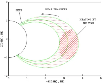
During magnetically disturbed conditions, large numbers of energetic particles are injected into the inner magnetosphere. These ring current particles are a major heat source for the thermal plasma in this region. Whereas the primary energy transfer channel from the hot ring current ions to the cool plasmaspheric particles is through Coulomb collisions (e.g. Cole, 1965; Kozyra et al., 1987; Fok et al., 1995; Kozyra et al., 1997; Liemohn et al., 2000; and references therein), wave particle interactions may also be important (e.g. Corn-wall et al., 1971; Hasegawa and Mima, 1978; Mishin and Burke, 2005; Gurgiolo et al., 2005; and references therein). In both cases the heating occurs preferentially near the equa-torial plane of the ring current. However, due to the high thermal conductivity of the electrons, soft particle precipi-tation and wave activity, part of this energy is carried along magnetic field lines down into the topside ionosphere; see Fig. 1. Accordingly, any satellite passing through the foot-point region of field lines threading the equatorial heating region should observe a sudden increase in the electron tem-perature. This is indeed the case. Figure 2 presents a se-quence of latitudinal profiles of the electron temperature as obtained by the Dynamics Explorer (DE)–2 satellite. The discontinuous increase in the temperature at subauroral lati-tudes is evident. In what follows, this remarkable feature will be called “subauroral electron temperature enhancement”.

Subauroral electron temperature enhancements were first identified by Norton and Findlay (1969), Chandra et al. (1971), Roble et al. (1971) and Raitt (1974) and were

(3)

1872 G. W. Pr¨olss: Subauroral electron temperature enhancement in the nighttime ionosphere

Fig. 1. Topology of magnetic field lines threading the inner-magnetospheric heating region. A projection onto the x–z plane of a geocentric solar-magnetospheric (GSM) coordinate system is shown. The field lines were calculated for 05.3 UT on 5 Septem-ber 1982 using the Tsyganenko model T 96-1. The footpoints are located at 53.5, 56.6 and 58.4 invariant latitude, respectively. They apply to the fifth subaural electron temperature enhancement shown in Fig. 2. RC stands for ring current and SET E for subauroral elec-tron temperature enhancement.

considered a storm phenomenon. Later, it was realized that these heating effects are a quasi-permanent feature of the plasmasphere and topside ionosphere (e.g. Brace and Theis, 1974; Brinton et al., 1978; Brace et al., 1982). Their mean properties were subsequently investigated by B¨uchner et al. (1983), Kozyra et al. (1986), Brace et al. (1988) and Fok et al. (1991a, b). It was discovered that the location and magnitude of the temperature enhancement depend on the level of geomagnetic activity, height and season. Here we supplement these studies. Using a much larger data set, we are able to describe the location of the equatorward bound-ary of the heating effect, identify local time variations, de-rive mean height and latitudinal profiles, document correla-tions with the ionospheric trough and subauroral ion drifts, and describe stormtime behaviour. The material to be pre-sented is organized in the following way. First, data selec-tion and processing are discussed (Sect. 2). Next, the loca-tion of the temperature enhancement and its dependence on geomagnetic activity and magnetic local time are determined (Sect. 3). Variations in the magnitude of the temperature en-hancement with altitude and geomagnetic activity are con-sidered in Sect. 4. A mean latitudinal profile of the heating effect is derived in Sect. 5. Its correlation with electron den-sity and ion drift speed is documented in Sect. 6. In Sect. 7, storm-induced modifications are considered. Finally, our ob-servations are compared with previous findings (Sect. 8), and the main results of our study are summarized in Sect. 9.

2 Data selection and their parameterization

The present study uses electron temperature and density mea-surements obtained by the Langmuir probe aboard the DE-2 satellite. A general description of this satellite is presented by Hoffman and Schmerling (1981), and details on the Lang-muir probe experiment can be found in Krehbiel et al. (1981). First measurements obtained by this instrument are discussed in Brace et al. (1982). In this study the DE-2 data sets pre-pared by the NASA National Space Science Data Center are analysed.

In order to record subauroral electron temperature en-hancements in a systematic way, all DE-2 orbits were di-vided into four segments, each extending from equatorial to polar latitudes. Of these segments, only those located in the night sector between 21:00 and 03:00 h magnetic local time were retained. Also, all passes with insufficient data cov-erage were removed from the data set. For each of the se-lected orbital segments, the electron temperature was plotted as a function of invariant latitude and displayed on a termi-nal screen. An inspection of these plots showed that in a few cases no temperature enhancements could be detected. In other cases, the temperature fluctuated so much that an un-ambiguous identification of the heating effect was not possi-ble. These passes were also removed from the data set.

The remaining profiles were then used to roughly parame-terize the subauroral heating effect. The latitude of the equa-torward boundary of the temperature enhancement, lat b, was estimated for each profile; see Fig. 2. The associated temper-ature value is denoted here by T eb. Likewise, the latitude lat mof the first and most equatorward located temperature maximum was determined, as was the associated tempera-ture value T em. Note that we are not looking for the absolute temperature maximum or for isolated peaks. In fact, in quite a few cases the selected temperature peak is a secondary maximum not necessarily well separated from other and pos-sibly larger temperature peaks at higher latitudes. Evidently, our selection criteria emphasize the equatorward edge of the heating effect.

The big advantage of the parameterization used in the present study is that it is simple and robust. This means that anybody can reproduce the data set investigated here. A major disadvantage is that we may select features other than subauroral heating effects. In fact, there are indications that during longer periods of very low geomagnetic activ-ity, our parameterization identifies aurora-related tempera-ture enhancements instead. In order to avoid this as far as possible, we considered only data which were recorded at times when the Dst index was less than zero and the AE6 index (to be defined later) was larger than 100 nT. There were also cases when the observed temperature increase was due to solar radiation. Such cases were eliminated by requiring the solar zenith angle to be larger than 100 deg. Applying these selection criteria, a total of 1159 data sets remained, and these form the basis of the present analysis.

(4)

G. W. Pr¨olss: Subauroral electron temperature enhancement in the nighttime ionosphere 1873

Figure 2:

Latitudinal variation of the electron temperature in the subauroral region

during magnetically active conditions. In the upper part of the ﬁgure, the AE and Dst

indices are used to describe geomagnetic activity during three days in September 1982.

During this time, eight latitudinal proﬁles of the electron temperature were obtained by

the DE-2 satellite. They are shown in the form of a stack plot in the lower part of the

ﬁgure. The times of observation are indicated next to each proﬁle, and also by arrows in

the upper part of the ﬁgure. Dotted reference lines mark the 600 K temperature level.

The common temperature scale is indicated by an arrow on the left-hand side. Using

a constant temperature gradient of 1 K/km, all temperature measurements have been

adjusted to a common altitude of 350 km. This reference altitude lies within the range

of the actual observation heights. Solar local time of observation is approximately 24 h,

and the magnetic local time varies between 23 and 1 h. For each proﬁle, vertical blue

lines mark the latitudes of the equatorward boundary (= latb) and the ﬁrst maximum

(= latm) of the electron temperature enhancement. The associated temperatures are

denoted as T e(latb) = T eb and T e(latm) = T em, respectively.

3

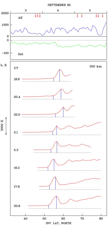
Fig. 2. Latitudinal variation of the electron temperature in the subauroral region during magnetically active conditions. In the upper part of the figure, the AE and Dst indices are used to describe geomagnetic activity during three days in September 1982. During this time, eight latitudinal profiles of the electron temperature were obtained by the DE–2 satellite. They are shown in the form of a stack plot in the lower part of the figure. The times of observation are indicated next to each profile, and also by arrows in the upper part of the figure. Dotted reference lines mark the 600 K temperature level. The common temperature scale is indicated by an arrow on the left-hand side. Using a constant temperature gradient of 1 K/km, all temperature measurements have been adjusted to a common altitude of 350 km. This reference altitude lies within the range of the actual observation heights. Solar local time of observation is approximately 24 h, and the magnetic local time varies between 23 and 1 h. For each profile, vertical blue lines mark the latitudes of the equatorward boundary (=latb) and the first maximum (=latm) of the electron temperature enhancement. The associated temperatures are denoted as T e(latb)=T eb and T e(lat m)=T em, respectively.

(5)

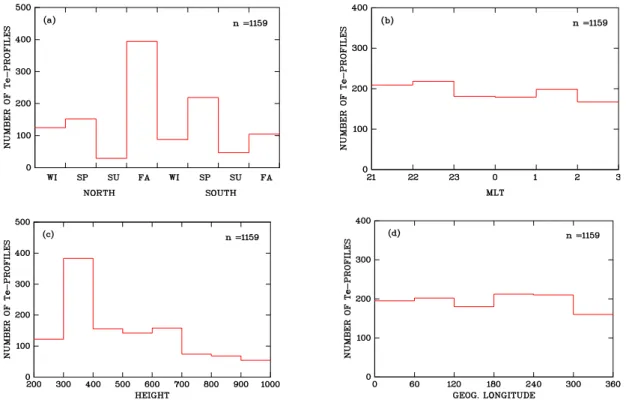
Fig. 3. Statistics of the data set analyzed in the present study. (a) Histogram indicating the hemispheric and seasonal distributions of 1159 parameterized electron temperature profiles. W I , SP , SU and F A stand for winter, spring, summer and fall, respectively. (b) Histogram indicating the magnetic local time (MLT ) distribution of the data set. (c) Histogram describing the height distribution of the data set. (d) Histogram indicating the longitudinal distribution of the data set.

The statistics of our data set are presented in Fig. 3. Evi-dently, more data were obtained in the Northern Hemisphere than in the Southern Hemisphere; see Fig. 3a. Also, there is a strong seasonal asymmetry, with most data referring to equinox conditions (70%) and only relatively few to summer conditions (<7%). As for the height distribution, most data were collected in the lower part of the upper ionosphere; see Fig. 3c. Finally, Figs. 3b and 3d indicate that both the mag-netic local time and longitude distributions of our data set are fairly even.

3 Location of the temperature enhancement

The location of the subauroral electron temperature enhance-ment is subject to considerable variations. These depend pri-marily on the level of geomagnetic activity. Here we describe and quantify these variations.

The latitudes of the equatorward boundary (latb) and first maximum (latm) of the temperature enhancement serve as convenient parameters to specify the location of the heating region. Selecting a suitable index to quantify the level of geomagnetic activity poses a greater problem. Various geo-magnetic activity indices were considered, including the Kp, Kp0, ap, AE, AE6 and Dst indices. Here, Kp0is the high-est Kp index during the 12-h period preceding the

respec-tive observation (e.g. Carpenter and Park, 1973). The use of Kp0 rather than Kp is in recognition that the response of the subauroral electron temperature enhancement to geo-magnetic activity may be delayed. Thus the position of the temperature enhancement may not only depend on the mo-mentary level of geomagnetic activity but also on its previ-ous history. This kind of “memory effect” is also taken into account by the AE6 index. It is defined as a weighted mean of the hourly-averaged AE indices for the actual hour and the previous 6 h:

AE6 = P6

i=0AE(U T − i[h])e−i

P6 i=0e−i

. (1)

Here UT refers to the universal time for which the AE6 in-dex is to be calculated (in our case the time of the electron temperature measurement). This index was found to be well correlated with the location of the trough minimum (Werner and Pr¨olss, 1997). Here we find that this index is also well correlated with the location of the subauroral electron tem-perature enhancement. In fact, the Dst and AE6 indices showed the highest correlations in this respect. Therefore, in what follows, only these two indices will be used.

In order to find out what kind of correlation exists between the Dst index and the location of the temperature enhance-ment, all lat m values were sorted into 10 nT wide intervals

(6)

Fig. 4. Position of the subauroral electron temperature enhancement as a function of geomagnetic activity. The Dst index is indicated on the abscissa, the invariant latitudes (L-shells) of the associated equatorward boundaries (latb) and maxima (latm) of the temper-ature enhancements on the ordinates. The median and the upper and lower quartiles of these parameters were determined for each 10 nT-wide interval of the Dst index. In the case of latm, these are indicated by the blue dots and bars. In the case of lat b, only the respective medians are shown (open blue circles). Linear regres-sion lines were fitted to the median values (latm: solid red line; lat b: dashed red line). The associated ordinate intersections a (in degrees) and slopes b (in degrees/nT) are given in the upper left-hand (lat m) and lower right-left-hand (lat b) corners, respectively. In both cases the correlation coefficient is greater than 0.98.

of this index. For each of these intervals, the median and the upper and lower quartiles of the latitude values were de-termined. They are indicated by the blue dots and bars in Fig. 4. As is evident, an excellent linear correlation exists between the Dst index and the latitude of the electron tem-perature maximum. Therefore, a linear regression line was fitted to the median values, and this is indicated by the solid red line. The associated line parameters are given in the up-per left-hand corner.

According to this regression line, the temperature peak is located slightly poleward of 60 deg invariant latitude during quiet conditions. For each decrease of the Dst index by 10 nT, the temperature peak moves towards lower latitudes by 0.8 deg. For a large geomagnetic storm of −300 nT, this would lead to an equatorward shift of 24 deg, and such large displacements are actually observed; see Sect. 7.

The same correlation analysis was also performed on the latitudes of the equatorward boundary of the heating region, i.e. latb. The regression line obtained in this case is indi-cated by the dashed red line. The respective line parameters

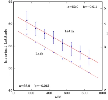
Fig. 5. Position of the subauroral electron temperature enhancement as a function of geomagnetic activity. The format of data presenta-tion corresponds to that of Fig. 4 except that this time the geomag-netic activity is indicated by the AE6 index. For a definition of this index see Eq. (1). The absolute magnitudes of the correlation coefficients are greater than 0.99.

are given in the lower right-hand corner. As can be seen, the equatorward boundary of the heating region and the temper-ature peak move at almost the same rate towards lower lati-tudes. The mean distance between latm and lat b is 3.6 deg.

The same mean distance is obtained if the Dst index is replaced by the AE6 index; see Fig. 5. In this case, both lat band lat m are displaced towards lower latitudes at a rate of about 1 deg per 100 nT increase in the AE6 index.

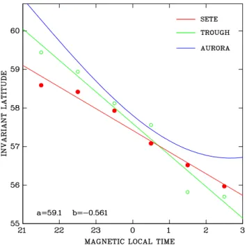
The location of the subauroral electron temperature en-hancement not only depends on the level of geomagnetic ac-tivity, but also on magnetic local time. To document this, correlation studies similar to Fig. 4 were performed for each 1-h interval of magnetic local time. Because of the smaller data sets, this time the regression lines were fitted directly to the individual data points. The results obtained for a Dst index of −43 nT are indicated by the red dots in Fig. 6. (The reason for choosing such a Dst value is explained below.) Going from the pre-midnight to the post-midnight sector, the temperature peak moves towards lower latitudes in a quasi-linear fashion, and this is emphasized by the regression line fitted to the data points. In the time interval considered, the total displacement is of the order of 3 deg, considerable less than the geomagnetic activity effect. Nevertheless, a clear asymmetry does exist in the position of the temperature en-hancement about midnight.

Similar asymmetries are also observed for other phenom-ena. Applying the same kind of analysis to a data set of

(7)

Fig. 6. Position of the subauroral electron temperature enhancement (SET E) as a function of magnetic local time. The red dots mark the mean position of the temperature peaks (=lat m) for each 1-h inter-val of magnetic local time during moderately strong geomagnetic activity (Dst = –43 nT, which corresponds to a Kp index of about 5). A linear regression line has been fitted to the data points (red line), and the associated fitting parameters are given in the lower left-hand corner (ordinate intersection a in degrees, slope b in de-grees/hour). The absolute magnitude of the correlation coefficient is almost 0.99. For comparison, we also show the corresponding mean values and regression line for the trough minimum (green cir-cles and green line). The blue line indicates the location of the equatorward boundary of the diffuse aurora for a Kp index of 5 (Gussenhoven et al., 1983).

trough minima compiled by Werner and Pr¨olss (1997), a magnetic local time variation as described by the green re-gression line in Fig. 6 is obtained. In addition, the blue line indicates the location of the equatorward boundary of the diffuse aurora as derived by Gussenhoven et al. (1983) for a Kp index of 5. Now a Kp index of 5 corresponds, ap-proximately, to a Dst index of −43 nT. This Dst value was therefore chosen to illustrate the magnetic local time vari-ations of the electron temperature enhancement and trough location. Of course, the same kind of local time asymmetry is also obtained for other levels of geomagnetic activity.

4 Magnitude of the temperature enhancement

Besides the location, the magnitude of the temperature en-hancement is of interest. It depends on both the altitude and the level of geomagnetic activity. A good way to document the height variation is to compare the mean height profiles of the electron temperature as observed at the locations of

Fig. 7. Height variation of the electron temperature at subauroral latitudes. Compared are mean height profiles of the electron tem-perature as observed at the location of the equatorward boundary (T eb) and the maximum (T em) of the heating region. For each 100 km-wide height interval, the median and the upper and lower quartiles of the temperature values were determined; see the blue dots and bars. Subsequently, fourth-order polynomials were fitted to the median values, and these are indicated by the red lines (see Eqs. (2) and (3)).

the equatorward boundary (T eb) and the maximum (T em) of the heating region; see Fig. 7. These mean height pro-files were determined as follows. First, all temperature val-ues were sorted into 100 km-wide height intervals. For each of these intervals, the median and the upper and lower quar-tiles of the temperature values were determined. They are indicated by the blue dots and bars in Fig. 7. Evidently, both T eband T em do increase with altitude, but at different rates. A simple analytical description of these height variations is obtained if a fourth-order polynomial is fitted to the medians

T eb =97 + 6.524 h − 1.410 · 10−2h2+1.456 · 10−5h3

−5.165 · 10−9h4 (2)

T em = −1249 + 23.84 h − 5.815 · 10−2h2+6.093 · 10−5h3

−2.152 · 10−8h4. (3)

Here T eb and T em are measured in Kelvin, and the height h in kilometer. These approximations are indicated by the red lines in Fig. 7. Now the magnitude of the temperature enhancement is simply the difference between the peak and the boundary temperatures, dT e=T em−T eb. Using the ap-proximations (Eqs. (2) and (3)), this quantity is plotted in

(8)

Fig. 8. Magnitude of the subauroral electron temperature enhance-ment as a function of altitude. Plotted is the difference between the temperatures observed at the location of the equatorward boundary and maximum of the heating region. This difference was deter-mined by subtracting Eq. (2) from Eq. (3).

Fig. 8. Note the striking increase in dT e above about 700 km altitude.

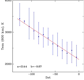
The magnitude of the temperature enhancement also de-pends on the level of geomagnetic activity. This is docu-mented in Figs. 9 and 10. Here the peak temperature T em serves as a convenient measure for the intensity of the sub-auroral heating, and the indices Dst and AE6 for the level of geomagnetic activity, respectively. In order to eliminate the height dependence of the heating effect, all T em val-ues were first adjusted to a common altitude of 600 km us-ing equation 3. A reference height of 600 km was chosen because this is approximately in the middle of the total alti-tude range considered here. The height-adjusted temperature values were then sorted into 10 nT-wide intervals of the Dst index and 100 nT-wide intervals of the AE6 index, respec-tively. For each of these subsets the median and the lower and upper quartiles were determined; see the blue dots and bars in Figs. 9 and 10. As indicated by the distance between the lower and upper quartiles, the scatter of the data points is substantial. Nevertheless, there is a clear trend for the peak temperature to increase with increasing geomagnetic activ-ity. To emphasize this, linear regression lines were fitted to the medians (red lines). The associated line parameters are given in the lower left- and right-hand corners, respectively.

As indicated in Fig. 9, the peak temperature T em increases by about 100 K for each decrease in the Dst index by 10 nT. Since 75% of our data were obtained during equinox condi-tions, this rate should be typical for this time of the year.

Fig. 9. Magnitude of the subauroral electron temperature enhance-ment as a function of geomagnetic activity. The Dst index is indi-cated on the abscissa, the associated peak temperature T em on the ordinate. All temperature values were adjusted to a common alti-tude of 600 km using the mean temperature profile shown in Fig. 7. The blue dots and bars indicate the medians and the upper and lower quartiles of the temperature values for each 10 nT-wide interval of the Dst index. Also shown is the regression line fitted to the medi-ans (red line). The associated line parameters are given in the lower left-hand corner (ordinate interception a in K, slope b in K/nT).

To check on this, the same correlation analysis was also performed separately on data sets obtained during winter, equinox and summer conditions. As indicated in Fig. 11, the equinox and summer results are similar to those presented in Fig. 10. However, the summer results may be affected by one of our selection criteria which requires the solar zenith angle to be larger than 100 deg. On the other hand, a signifi-cantly lower rate of increase (ca. 40 K per 10 nT decrease) is observed during winter conditions.

5 Mean latitudinal profile of the electron temperature enhancement

Calculating a mean latitudinal profile of the subauroral elec-tron temperature enhancement requires special care. This is because the rise in the electron temperature is confined to a relatively narrow latitudinal range whose position is constantly changing with the level of geomagnetic activity. Therefore simply averaging the individual profiles would in-variably smear out the heating effect. The result would be a mean temperature enhancement which is too broad and too small. To avoid this kind of distortion, a superposed epoch type of averaging procedure was used in the present study.

(9)

Fig. 10. Magnitude of the subauroral electron temperature enhance-ment as a function of geomagnetic activity. The format of data presentation is the same as in Fig. 9 except that the Dst index is replaced by the AE6 index.

Another difficulty arises from the height variation of the electron temperature and its dependence on latitude. For ex-ample, this height variation will be different inside and out-side the heating region. One way to circumvent this difficulty is to restrict the averaging to an altitude range in which the height variations are relatively small. In our case, this ap-plies for the height range between about 300 and 700 km; see Fig. 7. Accordingly, the following data processing procedure was adopted.

In a first step, all latitudinal profiles acquired below 300 km and above 700 km altitude were removed from the data set. Next, a linear regression analysis was performed to determine the temperature gradient between 300 and 700 km altitude for various latitudes inside and outside the heating region. At the location of the temperature maximum, this gradient was determined to be about 1 K/km; at the location of the equatorward boundary, it was about 0.8 K/km. Similar gradients were also obtained at lower latitudes. Therefore, a latitude-independent temperature gradient of 1 K/km was adopted. This gradient was then used to adjust all tempera-ture values to a common altitude of 500 km, which is in the middle of the height range considered here.

Next, all height-adjusted latitudinal profiles of the elec-tron temperature were superimposed in such a way that the maxima of the temperature enhancements were aligned and located at a common reference latitude (lat m → lat ref =0). This way the basic latitudinal structure of the heating effect is preserved when averaging the data. Subsequently, spline functions were fitted to each profile. This allowed us to

cal-Fig. 11. Seasonal variation of the subauroral electron temperature enhancement. The format of data presentation corresponds to that of Fig. 9 except that this time only the respective regression lines are shown. These regression lines refer to winter (blue line), equinox (green line) and summer (red line) conditions.

culate the temperatures at one degree steps relative to the new reference latitude. For each degree of this new coor-dinate system, the median and the upper and lower quartiles of the temperature values were determined. Finally, spline curves were fitted to these parameters. The end product of this whole procedure is presented in Fig. 12.

As indicated by the shaded area between the lower and upper quartiles, the scatter of the data is substantial. Never-theless, the mean electron temperature enhancement stands out as a relatively narrow peak, not unlike those actually ob-served. According to this mean profile, the temperature in-crease at 500 km altitude is about 1100 K, which corresponds to a relative increase of more than 75%. At half this maxi-mum value, the width of the temperature peak is approxi-mately 2.7 deg.

Note that the superposed epoch type of averaging proce-dure works well only near the common reference location. Thus the heating effects at auroral latitudes are invariably smeared out and not well described by our mean profile. Also note that the latitudes indicated on the abscissa refer to a Dst index of −50 nT. For this level of geomagnetic activity, the temperature peak is located at about 56.7◦invariant latitude; see Fig. 4. For other levels of activity, the latitude axis should be shifted to the right or left depending on whether the geo-magnetic activity is higher or lower.

(10)

Fig. 12. Mean latitudinal profile of the subauroral electron temperature enhancement at an altitude of 500 km. Plotted is the median of 841 temperature profiles. These profiles have been superimposed in such a way that the latitude of the temperature peak serves as a common reference location. The blue shaded area indicates the range between the lower and upper quartiles. Only data collected between 300 and 700 km altitude were considered. All temperature values were adjusted to a common height of 500 km using a constant temperature gradient of 1 K/km. The latitudes indicated on the abscissa apply for a Dst index of −50 nT (see last paragraph of this section).

Fig. 13. Mean latitudinal profiles of the subauroral electron tem-perature enhancement (red line) and the associated electron density (blue line). The format of data presentation is similar to that of Fig. 12 except that this time both data sets have been normalized using temperature and density values measured at the equatorward boundary of the heating region, i.e. T e(latb)=T eb and N e(latb), respectively. Also, only the latitudinal variation of the median val-ues is shown. As before, all data have been adjusted to a common altitude of 500 km, and only data collected in the height range 300 to 700 km are considered. Again, the latitudes indicated on the ab-scissa refer to a Dst index of −50 nT.

6 Electron density and ion drift velocity in the heating region

How does the electron density behave at the location of the temperature enhancement? If individual satellite passes are considered, sometimes increases (16% of all cases), more often decreases (84% of all cases) are observed. These trough-related decreases are sometimes exactly co-located with the temperature enhancement. More often, however, they are slightly displaced towards higher or lower latitudes.

Fig. 14. Mean latitudinal profiles of the subauroral electron tem-perature enhancement (red line) and the associated zonal ion drift speed (blue line). The format of data presentation corresponds to that of Fig. 13 except that the electron density is replaced by the absolute value of the zonal ion drift velocity.

To derive the mean relationship between both quantities, the data were processed in the following way.

As in Sect. 5, only the height interval between 300 and 700 km was considered. Within this height range, the elec-tron temperature and density data were adjusted to a com-mon reference altitude of 500 km. As before, this was done to eliminate changes which result from differences in the ob-servation heights. Again a constant temperature gradient of 1 K/km was adopted. In the case of the electron density, a barometric height distribution was assumed. The respective scale heights were calculated using the measured ion and electron temperatures. In case the ion temperature data were missing, this parameter was estimated using a formula sug-gested by Titheridge (1993).

(11)

Fig. 15. Latitudinal variation of the electron temperature during storm conditions. In the upper part of the figure, the AE and Dst indices are used to describe the geomagnetic activity during the storm of 6 September 1982. During the main phase of this storm, electron temperature profiles were obtained by the DE-2 satellite in both hemispheres. These profiles are shown in the lower part of the figure. The approximate universal times of the observations are in-dicated next to each profile, and also by an arrow in the AE panel of the figure. The dotted reference lines mark the 1000 K level, and the temperature scale is indicated by an arrow on the left-hand side. Using a constant temperature gradient of 1 K/km, all temperature values have been adjusted to a common altitude of 350 km. Solar local time of observation is approximately 24 h and the magnetic local time about 23 h. See also Fig. 2.

Next, the height-adjusted electron temperature and density data were normalized. This facilitates a comparison between the variations of both quantities. Here the temperature and density values measured at the equatorward boundary of the heating region (i.e. T e(latb)=T eb and N e(lat b)) served as convenient normalization standards.

Finally, the height-adjusted and normalized latitudinal profiles of the electron temperature and density were aver-aged. Again a superposed-epoch type of averaging procedure was used; see Sect. 5. For both quantities, the latitude of the

Fig. 16. Largest displacement of the subauroral electron tempera-ture enhancement towards lower latitudes as observed in the DE-2 data set. The format of data presentation corresponds to that of Fig. 15. This time, however, the dotted reference lines mark the 1200 K temperature level. Also, a constant temperature gradient of 2.5 K/km was used in the height adjustment procedure. Solar and magnetic local time of observation are approximately 03 h and 02 h, respectively. Both profiles were obtained in the Southern Hemi-sphere.

maximum electron temperature lat m served as a common reference location.

The end product of this data processing procedure is dis-played in Fig. 13. Evidently, the electron temperature en-hancement and the ionospheric trough are exactly co-located, on average.

The same procedure was also used to compare the latitudi-nal variation of the electron temperature with those of the ion temperature, the neutral gas temperature and the neutral gas composition (= atomic oxygen to molecular nitrogen density ratio). No correlations were observed. Only the zonal ion drift speed showed a significant increase right at the location of the electron temperature peak, and this is documented in Fig. 14.

(12)

7 Large-storm effects

Following a period of moderate activity, a large geomagnetic storm occurred on 6 September 1982; see upper panel of Fig. 15. Shortly after the Dst index reached its minimum value of −289 nT, two latitudinal profiles of the electron temperature were recorded by the DE-2 satellite; see lower panel of Fig. 15. One was obtained in the Northern Hemi-sphere, the other one in the Southern Hemisphere. As can be seen, in both cases the temperature perturbations set in at exactly the same latitude, as would be expected from the heating scenario depicted in Fig. 1. Within the perturbation zone itself, somewhat different temperature variations are ob-served. This is attributed here to the different ionospheric conditions in both hemispheres.

Comparing the stormtime profiles with those observed during the prestorm phase (see Fig. 2), the following differ-ences are noted. During the storm, the temperature perturba-tions are larger and extend towards lower latitudes. This is, of course, what is to be expected from our statistical analy-sis. More interesting is that during a major storm the local minimum between the subauroral electron temperature peak and the heating effects at higher latitudes is filled in. Accord-ingly, the stormtime profiles look more like step functions.

This is typical for storm conditions although exceptions are observed; see lower temperature profile in Fig. 16. This profile documents the largest displacement of the subauroral electron temperature enhancement towards lower latitudes observed in our data set. Whereas the onset of the distur-bance is located below 35 deg, the temperature peak is ob-served near 36 deg invariant latitude. This corresponds to an L-shell value of less than 1.6!

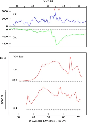
Residual temperature enhancements observed during the recovery phase of a geomagnetic storm are another feature of interest. Figure 17 presents an example of this effect. Here we are interested in the two lower-most temperature profiles observed in the early morning hours of 9 August 1982. At this time there was no substorm activity and the ring current had almost – but not completely – recovered to prestorm con-ditions. Evidently, the residuals of the ring current created on 7 August were still sufficient to heat the topside ionosphere significantly. One characteristic feature of these late heating effects is that the temperature varies much more smoothly than during magnetically active conditions.

8 Comparison with previous results and discussion

In the preceding sections, some properties of the temper-ature enhancement at subauroral latitudes were described. Here these observations will be discussed and compared with previous findings.

Fig. 17. Residual heating effects during a period of low geomag-netic activity. The format of data presentation corresponds to that of Fig. 15. This time the dotted reference lines mark the 700 K tem-perature level. Also, a constant temtem-perature gradient of 1 K/km was used in the height adjustment procedure. The solar local time of ob-servation is 03.5 h, and the magnetic local time varies between 00.6 and 02.4 h.

8.1 Location of the temperature enhancement

It was recognized quite early that during geomagnetic storms the subauroral electron temperature enhancement moves

(13)

1882 G. W. Pr¨olss: Subauroral electron temperature enhancement in the nighttime ionosphere towards lower latitudes (Raitt, 1974; Brace et al., 1974). First

statistical investigations of this effect are due to Kozyra et al. (1986), Brace et al. (1988) and Fok et al. (1991a, b). Here we compare these previous findings with our present results. Such a comparison is not straight forward. First, these earlier studies used different criteria to identify the heating effects. Second, different indices were employed to describe the level of geomagnetic activity. Third, besides the invariant latitude, the L-shell parameter was used to specify the location of the heating effect. Nevertheless, keeping these differences in mind, some of the results may be set side by side. Here the studies by Kozyra et al. (1986) and Fok et al. (1991b) are of particular interest.

Kozyra et al. (1986) found that the location of the subauro-ral heating effect is better correlated with the Dst than with the Kp0_{index, and we certainly agree. Based on 206}

temper-ature peaks identified in the night sector, they also derived the following relationship between the location of these temper-ature peaks and the Dst index:

lat (T e peak) =60.02 + 0.055 Dst . (4)

This should be compared with our own result presented in Fig. 4:

lat m =60.7 + 0.080 Dst . (5)

Evidently, the agreement is reasonably good. In fact, both equations predict the heating effect to be located slightly poleward of 60◦invariant latitude for a Dst index of zero. And for a Dst index of −100 nT, the predicted locations dif-fer by less than 2 deg.

In the study by Fok et al. (1991b), it is suggested that the rate at which the temperature peak moves to-wards lower latitudes depends on season. Using our own data set, we also find a slightly larger displacement effect during equinox conditions (bequinox=0.083 deg/nT versus bsolst ice=0.073 deg/nT). This difference, however, is small

and may not be significant.

In Sect. 6 it was shown that, on average, the subauro-ral electron temperature enhancement and the ionospheric trough are co-located. This implies that the locations of both phenomena should depend on the level of geomagnetic ac-tivity in a similar way. According to the models A and B of Werner and Pr¨olss (1997), at midnight (00 MLT) the trough minimum (TM) should be located at

Model A : lat T M(00 MLT)=63.5−0.016 AE6 (6) Model B : lat T M(00 MLT)=63.3−0.017 AE6 . (7) Our present results predict the electron temperature enhance-ment to be located at

lat m =62 − 0.011 AE6 , (8)

see Fig. 4. As is evident, the agreement is quite good, at least for moderately disturbed conditions.

In the study by Brace et al. (1988), it is suggested that the location of the poleward edge of the subauroral electron tem-perature enhancement is roughly independent of magnetic local time. Here we find that the location of the tempera-ture peak clearly varies with magnetic local time, at least in the night sector. We also demonstrate that the observed po-sitional asymmetry around midnight is nothing unusual and that it is also observed for other phenomena like the iono-spheric trough and the equatorward boundary of the diffuse aurora; see Fig. 6.

Whereas the location of the subauroral electron tempera-ture enhancement is of intrinsic interest in itself, it may also be important for magnetospheric physics. This is because this heating effect represents a sensitive marker of inner-magnetospheric energy transfer processes (e.g. Fok et al., 1995; Kozyra et al., 1997; Liemohn et al., 2000). In fact, if the dominant energy source of the heating effect is Coulomb collisions of ring current ions with plasmaspheric electrons, the equatorward boundary of the electron temperature en-hancement could be used to trace the location of the inner edge of the ring current. Assuming that such a connection exists, the inner boundary of the ring current would some-times be located surprisingly close to Earth. For example, during the large storm of 14 July 1982, when the equatorward boundary of the temperature enhancement was observed near 35◦invariant latitude, the ring current should have penetrated to an L-shell as low as 1.5!

8.2 Magnitude of the temperature enhancement

Heat transfer from the ring current to the ionosphere requires a positive temperature gradient in the topside ionosphere. For the location of the subauroral electron temperature en-hancement, this gradient was first estimated by B¨uchner et al. (1983). Fitting linear regression lines to their data sets, they obtained nighttime temperature gradients of the order of 0.33 and 1.05 K/km, depending on the level of geomagnetic activity. Substantially larger temperature gradients (1.4 to 3 K/km) were subsequently derived by Kozyra et al. (1986).

Our data set allows a more detailed investigation of this height variation. As it turns out, the temperature gradient is all but constant; see Fig. 7. In particular, there is a con-spicuous increase in this gradient above about 700 km al-titude. According to Cole (2003), this is what one should expect. Assuming no net field-aligned currents in the mag-netic flux tubes connecting the ring current region with the ionosphere, he derives temperature gradients for the upper topside ionosphere; these gradients are up to several degrees per kilometer larger than predicted by conventional theory. Evidently, our results are in agreement with this new heat transport model.

In addition to altitude, the magnitude of the subauroral temperature enhancement also depends on the level of geo-magnetic activity (B¨uchner et al., 1983; Kozyra et al., 1986; Fok et al., 1991 a, b; and Figs. 9 and 10 of our present

(14)

G. W. Pr¨olss: Subauroral electron temperature enhancement in the nighttime ionosphere 1883 investigation). Since all these studies are based on

differ-ent data sets, only a rough comparison is possible. For ex-ample, the rates at which the peak temperature increases with decreasing Dst index varies in these studies between −8.1 K/nT (B¨uchner et al.), −8.0 and −23.3 K/nT, depend-ing on altitude (Kozyra et al.), −7.8 and −14.2 K/nT, de-pending on season (Fok et al.), and −9.9 K/nT (present study). It is reassuring that apart from the −23.3 K/nT value, all rates are of the same order of magnitude. Whereas we do not find this rate to depend on altitude, the seasonal varia-tions suggested by Fok et al. (1991b) are also seen in our data set, at least regarding the lower rate observed during winter conditions; see Fig. 11.

8.3 Mean latitudinal profiles

The first to derive mean latitudinal profiles of the electron temperature in the night sector was Titheridge (1976). Ex-cept for a general increase, no indication of a discontinu-ous temperature enhancement at subauroral latitudes was ob-served. Considering the low latitudinal resolution of the data set at his disposal and the averaging procedure employed, this is not surprising. The difficulty of deriving such mean profiles without washing out small scale structures was em-phasized by Brace (1990).

Here a superposed epoch type of averaging procedure is used (see also Pr¨olss, 2006). In this case, the subauroral electron temperature enhancement stands out as an isolated peak, not unlike those actually observed; see Fig. 12. The mean temperature increase is of the order of 1100 K, and this corresponds to a relative increase of more than 75%; see also Figs. 8 and 13. The width of the temperature peak at half this maximum value is about 2.7 deg. Also the distance between the equatorward boundary and the maximum is 3 to 4 deg, in good agreement with our statistical result (3.6 deg).

There are a number of possible applications for such a mean temperature profile. For example, it may be incorpo-rated into empirical models of the ionosphere. So far, none of these models, including the International Reference Iono-sphere (IRI; see Bilitza, 2001) contains a specification of the subauroral electron temperature enhancement.

Another application would be to compare it to the lati-tudinal variations of other quantities. For example, it was realized early that the mid-latitude ionospheric trough and the subauroral electron temperature enhancement are closely coupled phenomena (e.g. Moffett and Quegan, 1983; Hor-witz et al., 1986; Watanabe et al., 1989; Afonin et al., 1997; Karpachev et al., 1997; Karpachev and Afonin, 2004; and references therein). Whereas these studies contain numerous examples of this coupling, their mean correlation is docu-mented for the first time in Fig. 13. It is found that, on av-erage, the electron temperature enhancement and the trough-related electron density decrease are exactly co-located.

The physics behind this close coupling is incompletely un-derstood. Given a local increase in the heat flux from above,

this will certainly enhance the electron temperature. This temperature enhancement, in turn, will increase the loss rate of electrons, and a trough will form. On the other hand, the electron density may be reduced by some other mechanism. In this case, even a smoothly varying heat flux will cause a localized temperature enhancement. This is because each electron in the trough region will get a larger share of the heat addition. Moreover, the heat loss will be smaller be-cause of the lower ion density. A more detailed discussion of this topic is beyond the scope of this paper, and the interested reader is referred to the pertinent literature (e.g. Pavlov, 2000; Mishin et al., 2004; Sojka et al., 2004; Wang et al., 20061; and references therein).

One of the mechanisms which may reduce the ionization density in the trough region is increased ion convection. And indeed, a moderate increase in ion drift speed is observed at the location of the electron temperature enhancement; see Fig. 14. At the same time, no increase in ion temperature is observed. This indicates that the mean increase in ion drift speed (ca. 110 m/s) is too small to affect the ion temperature in a significant way. On the other hand, there are numer-ous examples when enhanced electron temperatures and den-sity troughs are observed in regions of high ion drift speeds and high ion temperatures, especially during more strongly disturbed conditions (e.g. Foster et al., 1994; Moffett et al., 1998; F¨orster et al., 1999; Wang et al., 20061; and references therein). Therefore any generalization should be considered with due caution.

8.4 Storm effects

It was recognized early that during geomagnetic storms the subauroral electron temperature enhancement increases in magnitude and moves towards lower latitudes (e.g. Raitt, 1974; Brace et al., 1974; Afonin et al., 1997; Karpachev and Afonin, 2004). Our data are certainly in agreement with these findings. We add that during large geomagnetic storms the heating effect (and by inference the inner edge of the ring current) may be observed at rather low latitudes (<35◦) and L-shells (<1.5); see Fig. 16.

We also note that the shape of the latitudinal profile of the heating effect changes during major storms. Instead of being marked by a more or less isolated temperature peak at the equatorial boundary of the heating zone, storm profiles often look more like step functions. As to be expected, these heat-ing effects are conjugate phenomena (see Fig.15), although data to confirm this expectation seem to be scarce.

It was also noted early that following larger geomagnetic storms, the subauroral heating effects may persist for many hours, even days, long after the substorm activity had ceased (Raitt, 1974; Horwitz et al., 1986; Karpachev, 2001). Evi-dently, the ring current as a heat source exists much longer

1_{Wang, W., Burns, A. G., and Killeen, T. L.: A numerical study}

of the response of ionospheric electron temperature to geomagnetic activity, J. Geophys. Res., submitted, 2006.

(15)

1884 G. W. Pr¨olss: Subauroral electron temperature enhancement in the nighttime ionosphere than the magnetospheric activity responsible for its

forma-tion. Again, our data are in agreement with these find-ings. We add that such residual effects are marked by rather smooth latitudinal profiles.

9 Summary of observations

In the nighttime subauroral ionosphere, a quasi-permanent discontinuous increase in the electron temperature is ob-served. Using DE-2 satellite data, the main properties of this remarkable feature are investigated. These may be summa-rized as follows.

– During moderately disturbed conditions, a relatively

narrow peak in the electron temperature is observed at subauroral latitudes. At 500 km altitude, this tempera-ture enhancement is of the order of 1100 K, on average, which corresponds to a relative increase of more than 75%. At half this peak value, the width of the tempera-ture enhancement is about 2.7 deg. Also, the mean dis-tance between the equatorward boundary of the temper-ature enhancement and the location of the t empertemper-ature peak is found to be 3.6 deg.

– The magnitude of the temperature enhancement varies

with altitude. Within the height range 280 to 940 km, it increases by 73%, on average. Thereby a conspicu-ous increase in the temperature is observed above about 700 km altitude. The magnitude of the temperature en-hancement also depends on the level of geomagnetic ac-tivity. For a decrease in the Dst index by 100 nT, an increase of 46% in the peak temperature is observed. This rate of increase, however, depends on season, with smaller increases observed during winter conditions.

– The location of the temperature enhancement is

primar-ily controlled by the level of geomagnetic activity. Dur-ing quiet conditions (Dst'0), the temperature peak is located slightly poleward of 60◦invariant latitude. For each decrease of the Dst index by 10 nT it moves equa-torward by 0.9◦, on average. The location of the temper-ature enhancement also depends on magnetic local time. Before midnight, the temperature peak is observed at higher latitudes, past midnight at lower latitudes.

– In general, a decrease in the electron density and an

in-crease in the zonal ion drift speed are observed at the lo-cation of the temperature enhancement. No correlation with the ion and neutral gas temperatures or the neutral gas composition is found.

– During major geomagnetic storms, the latitudinal

pro-files of the temperature enhancements assume more step-function-like shapes. Also, the heating effects may extend to very low latitudes (less than 35◦invariant lat-itude). And, residual heating effects are observed long after the storm-substorm activity has ceased.

The nightside subauroral region is not the only place where significant increases in the electron temperature of the topside ionosphere are observed. In fact, similar peaks in the electron temperature are also recorded in the dayside po-lar ionosphere beneath the magnetospheric cusp. The mean properties of this latter phenomenon are investigated in a study by Pr¨olss (2006).

Acknowledgements. The DE-2 data used in this study were kindly

provided by the NASA National Space Science Data Center. I am grateful to all the experimenters who contributed to this data set. I am also indebted to N. Tsyganenko and S. Werner for their advice in programming matters. Finally, I would like to thank K. Schr¨ufer and M. Hanussek for their help in preparing this manuscript.

Topical Editor M. Pinnock thanks D. Bilitza and M. C. Fok for their help in evaluating this paper.

References

Afonin, V. V., Bassolo, V. S., Smilauer, J., and Lemaire, J. F.: Mo-tion and erosion of the nightside plasmapause region and of the associated subauroral electron temperature enhancement: Cos-mos 900 observations, J. Geophys. Res., 102, 2093–2103, 1997. Bilitza, D.: International Reference Ionosphere 2000, Radio Sci.,

36, 261–275, 2001.

Brace, L. H.: Solar cycle variations in F-region Te in the vicinity of the midlatitude trough based on AE-C measurements at so-lar minimum and DE-2 measurements at soso-lar maximum, Adv. Space Res., 10, (11)83–(11)88, 1990.

Brace, L. H. and Theis, R. F.: The behavior of the plasmapause at mid-latitudes: Isis 1 Langmuir probe measurements, J. Geophys. Res., 79, 1871–1884, 1974.

Brace, L. H., Maier, E. J., Hoffman, J. H., Whitteker, J., and Shep-herd, G. G.: Deformation of the night side plasmasphere and ionosphere during the August 1972 geomagnetic storm, J. Geo-phys. Res., 79, 5211–5218, 1974.

Brace, L. H., Theis, R. F., and Hoegy, W. R.: A global view of the F-region electron density and temperature at solar maximum, Geophys. Res. Lett., 9, 989–992, 1982.

Brace, L. H., Chappell, C. R., Chandler, M. O., Comfort, R. H., Horwitz, J. L., and Hoegy, W. R.: F region electron temperature signatures of the plasmapause based on Dynamics Explorer 1 and 2 measurements, J. Geophys. Res., 93, 1896–1908, 1988. Brinton, H. C., Grebowsky, J. M., and Brace, L. H.: The

high-latitude winter F region at 300 km: Thermal plasma observations from AE-C, J. Geophys. Res., 83, 4767–4776, 1978.

B¨uchner, J., Lehmann, H.-R., and Rendtel, J.: Properties of the sub-auroral electron temperature peak observed by Langmuir-probe measurements on board Intercosmos-18, Gerlands Beitr. Geo-phys., 92, 368–372, 1983.

Carpenter, D. L. and Park, C. G.: On what ionospheric workers should know about the plasmapause-plasmasphere, Rev. Geo-phys. Space Phys., 11, 133–154, 1973.

Caton, R., Horwitz, J. L., Richards, P. G., and Liu, C.: Model-ing of F-region ionospheric upflows observed by EISCAT, Geo-phys.Res.Lett., 23, 1537–1540, 1996.

(16)

G. W. Pr¨olss: Subauroral electron temperature enhancement in the nighttime ionosphere 1885 Chandra, S., Maier, E. J., Troy Jr., B. E., and Narasinga Rao, B.

C.: Subauroral red arcs and associated ionospheric phenomena, J. Geophys. Res., 76, 920–925, 1971.

Cole, K. D.: Stable auroral red arcs, sinks for energy of Dst main phase, J. Geophys. Res., 70, 1689–1706, 1965.

Cole, K. D.: Return current and heat transport into zero-order SAR arcs, J. Atmos. Solar-Terr. Phys., 65, 787–799, 2003.

Cornwall, J. M., Coroniti, F. V., and Thorne, R. M.: Unified theory of SAR arc formation at the plasmapause, J. Geophys. Res., 76, 4428–4445, 1971.

Fok, M.-C., Kozyra, J. U., and Brace, L. H.: Solar cycle variation in the subauroral electron temperature enhancement: Comparison of AE-C and DE 2 satellite observations, J. Geophys. Res., 96, 1861–1866, 1991a.

Fok, M.-C., Kozyra, J. U., Warren, M. F., and Brace, L. H.: Sea-sonal variations in the subauroral electron temperature enhance-ment, J. Geophys. Res., 96, 9773–9780, 1991b.

Fok, M.-C., Craven, P. D., Moore, T. E., and Richards, P. G.: Ring current-plasmasphere coupling through coulomb collisions, in: Cross-Scale Coupling in Space Plasmas, edited by: Horwitz, J. L., Singh, N., and Burch, J. L., AGU monogr. 93, 161–171, 1995. Foster, J. C., Buonsanto, M. J., Mendillo, M., Nottingham, D., Rich, F. J., and Denig, W.: Coordinated stable auroral red arc observa-tions: Relationship to plasma convection, J. Geophys. Res., 99, 11 429–11 439, 1994.

F¨orster, M., Foster, J. C., Smilauer, J., Kudela, K., and Mikhailov, A. V.: Simultaneous measurements from the Millstone Hill radar and the Active satellite during the SAID/SAR arc event of the March 1990 CEDAR storm, Ann. Geophys., 17, 389–404, 1999. Gurgiolo, C., Sandel, B. R., Perez, J. D., Mitchell, D. G., Pollock, C. J., and Larsen, B. A.: Overlap of the plasmasphere and ring current: Relation to subauroral ionospheric heating, J. Geophys. Res., 110, A12217, doi:10.1029/2004JA010986, 2005.

Gussenhoven, M. S., Hardy, D. A., and Heinemannm N.: System-atics of the equatorward diffuse auroral boundary, J. Geophys. Res., 88, 5692–5708, 1983.

Hasegawa, A. and Mima, K.: Anomalous transport produced by ki-netic Alfven wave turbulence, J. Geophys. Res., 83,, 1117–1123, 1978.

Hoffman, R. A. and Schmerling, E. R.: Dynamics Explorer pro-gram: An overview, Space Sci. Instr., 5, 345–348, 1981. Horwitz, J. L., Brace, H. C., Comfort, R. H., and Chappell, C. R.:

Dual-spacecraft measurements of plasmasphere-ionosphere cou-pling, J. Geophys. Res., 91, 11 203–11 216, 1986.

Karpachev, A. T.: Characteristics of the ring ionospheric trough, Geomag. Aeron., 41, 55–64, 2001.

Karpachev, A. T. and Afonin, V. V.: Variations in the structure of the high-latitude ionosphere during the March 22-23, 1979, storm based on Cosmos-900 and Intercosmos-19 data, Geomag. Aeron., 44, 60–68, 2004.

Karpachev, A. T., Afonin, V. V., and Smilauer, J.: Electron-temperature distribution near the ionospheric trough for summer nighttime conditions, Geomag. Aeron., 37, 67–72, 1997. Kozyra, J. U., Brace, L. H., Cravens, T. E., and Nagy, A. F.: A

statistical study of the subauroral electron temperature enhance-ment using Dynamics Explorer 2 Langmuir probe observations, J. Geophys. Res., 91, 11 270–11 280, 1986.

Kozyra, J. U., Cravens, T. E., Nagy, A. F., Gurnett, D. A., Huff, R. L., Comfort, R. H., Waite Jr., J. H., Brace, L. H., Winningham,

J. D., Burch, J. L., and Peterson, W. K.: Satellite observations of new particle and field signatures associated with SAR arc field lines at magnetospheric heights, Adv. Space Res., 7, (8)3–(8)6, 1987.

Kozyra, J. U., Nagy, A. F., and Slater, D. W.: High-altitude energy source(s) for stable auroral red arcs, Rev. Geophys., 35, 155–190, 1997.

Krehbiel, J. P., Brace, L. H., Theis, R. F., Pinkus, W. H., and Ka-plan, R. B.: The Dynamics Explorer Langmuir probe instrument, Space Sci. Instr., 5, 493–502, 1981.

Liemohn, M. W., Kozyra, J. U., Richards, P. G., Khazanov, G. V., Buonsanto, M. J., and Jordanova, V. K.: Ring current heating of the thermal electrons at solar maximum, J. Geophys. Res., 105, 27 767–27 776, 2000.

Mishin, E. V. and Burke, W. J.: Stormtime coupling of the ring current, plamasphere, and topside ionosphere: Electromag-netic and plasma disturbances, J. Geophys. Res., 110, A07209, doi:10.1029/2005JA011021, 2005.

Mishin, E. V., Burke, W. J., and Viggiano, A.A.: Stormtime subau-roral density troughs: Ion-molecule kinetics effects, J. Geophys. Res., 109, A10301, doi:10.1029/2004JA010438, 2004.

Moffett, R. J. and Quegan, S.: The mid-latitude trough in the elec-tron concentration of the ionospheric F-layer: A review of obser-vations and modelling, J. Atmos. Terr. Phys., 45, 315–343, 1983. Moffett, R. J., Ennis, A. E., Bailey, G. J., Heelis, R. A., Brace, L. H.: Electron temperatures during rapid subauroral ion drift events, Ann. Geophys., 16, 450–459, 1998.

Norton, R. B. and Findlay, J. A.: Electron density and temperature in the vicinity of the 29 September 1967 middle latitude red arc, Planet. Space Sci., 17, 1867–1877, 1969.

Pavlov, A. V.: Dependence of the electron temperature in the sub-auroral red arc region on electron density and the heat flux from the plasmasphere, Geomag. Aeron., 40, 339–343, 2000. Pr¨olss, G. W.: Electron temperature enhancement beneath the

mag-netospheric cusp, J. Geophys. Res., in press, 2006.

Raitt, W. J.: The temporal and spatial development of mid-latitude thermospheric electron temperature enhancements during a geo-magnetic storm, J. Geophys. Res., 79, 4703–4708, 1974. Roble, R. G., Norton, R. B., Findlay, J. A., and Marovich, E.:

Calculated and observed features of stable auroral red arcs dur-ing three geomagnetic storms, J. Geophys. Res., 76, 7648–7662, 1971.

Sojka, J. J., David, M., Schunk, R. W., Foster, J. C., and Vo, H. B.: A modeling study of the F-region response to SAPS, J. Atmos. Solar-Terr. Phys., 66, 415–423, 2004.

Titheridge, J. E.: Plasmapause effects in the top side ionosphere, J. Geophys. Res., 81, 3227-3233, 1976.

Titheridge, J. E.: Atmospheric winds calculated from diurnal changes in the midlatitude ionosphere, J. Atmos. Terr. Phys., 55, 1637–1659, 1993.

Watanabe, S., Oyama, K.-I., and Abe, T.: Electron temperature structure around mid latitude ionospheric trough, Planet.Space Sci., 37, 1453–1460, 1989.

Werner, S., and Pr¨olss, G. W.: The position of the ionospheric trough as a function of local time and magnetic activity, Adv. Space Res., 20, No. 9, 1717–1722, 1997.