HAL Id: hal-01149834
https://hal.archives-ouvertes.fr/hal-01149834
Submitted on 7 May 2015
HAL is a multi-disciplinary open access
archive for the deposit and dissemination of
sci-entific research documents, whether they are
pub-lished or not. The documents may come from
teaching and research institutions in France or
abroad, or from public or private research centers.
L’archive ouverte pluridisciplinaire HAL, est
destinée au dépôt et à la diffusion de documents
scientifiques de niveau recherche, publiés ou non,
émanant des établissements d’enseignement et de
recherche français ou étrangers, des laboratoires
publics ou privés.
On the Super-Additivity and Estimation Biases of
Quantile Contributions
Nassim Nicholas Taleb, Raphaël Douady
To cite this version:
Nassim Nicholas Taleb, Raphaël Douady. On the Super-Additivity and Estimation Biases of Quantile
Contributions. 2014. �hal-01149834�
Centre d’Economie de la Sorbonne
On the Super-Additivity and Estimation Biases
Of Quantile Contributions
Nassim Nicholas T
ALEB,Raphaël D
OUADY2014.90
Maison des Sciences Économiques, 106-112 boulevard de L'Hôpital, 75647 Paris Cedex 13
http://centredeconomiesorbonne.univ-paris1.fr/
EXTREME RISK INITIATIVE —NYU SCHOOL OF ENGINEERING WORKING PAPER SERIES
On the Super-Additivity and Estimation Biases of
Quantile Contributions
Nassim Nicholas Taleb
∗, Raphael Douady
†∗
School of Engineering, New York University
†
Riskdata & C.N.R.S. Paris, Labex ReFi, Centre d’Economie de la Sorbonne
Abstract—Sample measures of top centile contributions to the total (concentration) are downward biased, unstable estimators, extremely sensitive to sample size and concave in accounting for large deviations. It makes them particularly unfit in domains with power law tails, especially for low values of the exponent. These estimators can vary over time and increase with the population size, as shown in this article, thus providing the illusion of structural changes in concentration. They are also inconsistent under aggregation and mixing distributions, as the
weighted average of concentration measures for A and B will
tend to be lower than that from A ∪ B. In addition, it can be
shown that under such fat tails, increases in the total sum need to be accompanied by increased sample size of the concentration measurement. We examine the estimation superadditivity and bias under homogeneous and mixed distributions.
Fourth version, Nov 11 2014
This work was achieved through the Laboratory of Ex-cellence on Financial Regulation (Labex ReFi) supported by PRES heSam under the reference ANR-10-LABX-0095.
I. INTRODUCTION
Vilfredo Pareto noticed that 80% of the land in Italy belonged to 20% of the population, and vice-versa, thus both giving birth to the power law class of distributions and the popular saying 80/20. The self-similarity at the core of the property of power laws [?] and [?] allows us to recurse and reapply the 80/20 to the remaining 20%, and so forth until one obtains the result that the top percent of the population will own about 53% of the total wealth.
It looks like such a measure of concentration can be seriously biased, depending on how it is measured, so it is very likely that the true ratio of concentration of what Pareto observed, that is, the share of the top percentile, was closer to 70%, hence changes year-on-year would drift higher to converge to such a level from larger sample. In fact, as we will show in this discussion, for, say wealth, more complete samples resulting from technological progress, and also larger population and economic growth will make such a measure converge by increasing over time, for no other reason than expansion in sample space or aggregate value.
The core of the problem is that, for the class one-tailed fat-tailed random variables, that is, bounded on the left and unbounded on the right, where the random variable X ∈ [xmin,∞), the in-sample quantile contribution is a biased estimator of the true value of the actual quantile contribution.
Let us define the quantile contribution κq = q
E[X|X > h(q)] E[X]
where h(q) = inf{h ∈ [xmin,+∞) , P(X > h) ≤ q} is the exceedance threshold for the probability q.
For a given sample(Xk)1≤k≤n, its "natural" estimator!κq ≡ qthpercentile
total , used in most academic studies, can be expressed, as !κq≡ "n i=1 Xi>ˆh(q)Xi "n i=1Xi
where ˆh(q) is the estimated exceedance threshold for the probability q: ˆ h(q) = inf{h : 1 n n # i=1 x>h≤ q}
We shall see that the observed variable !κq is a downward biased estimator of the true ratio κq, the one that would hold out of sample, and such bias is in proportion to the fatness of tails and, for very fat tailed distributions, remains significant, even for very large samples.
II. ESTIMATIONFORUNMIXEDPARETO-TAILED
DISTRIBUTIONS
Let X be a random variable belonging to the class of distributions with a "power law" right tail, that is:
P(X > x) ∼ L(x) x−α (1) where L : [xmin,+∞) → (0, +∞) is a slowly varying function, defined as limx→+∞L(kx)L(x) = 1 for any k > 0.
There is little difference for small exceedance quantiles (<50%) between the various possible distributions such as Student’s t, Lévy α-stable, Dagum,[?],[?] Singh-Maddala dis-tribution [?], or straight Pareto.
For exponents 1 ≤ α ≤ 2, as observed in [?], the law of large numbers operates, though extremely slowly. The problem is acute for α around, but strictly above 1 and severe, as it diverges, for α= 1.
A. Bias and Convergence
1) Simple Pareto Distribution: Let us first consider φα(x) the density of a α-Pareto distribution bounded from below by xmin>0, in other words: φα(x) = αxαminx−α−1 x≥xmin, and
P(X > x) =$xmin
x %α
. Under these assumptions, the cutpoint of exceedance is h(q) = xminq−1/α and we have:
κq = &∞ h(q)x φ(x)dx &∞ xminx φ(x)dx = 'h(q) xmin ( 1−α= qα−1 α (2) 1
If the distribution of X is α-Pareto only beyond a cut-point xcut, which we assume to be below h(q), so that we have P(X > x) = $λ
x %α
for some λ > 0, then we still have h(q) = λq−1/α and κq= α α− 1 λ E[X]q α−1 α
The estimation of κq hence requires that of the exponent α as well as that of the scaling parameter λ, or at least its ratio to the expectation of X.
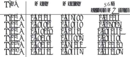
Table I shows the bias of !κq as an estimator of κq in the case of an α-Pareto distribution for α= 1.1, a value chosen to be compatible with practical economic measures, such as the wealth distribution in the world or in a particular country, including developped ones.1 In such a case, the estimator is extemely sensitive to "small" samples, "small" meaning in practice108. We ran up to a trillion simulations across varieties of sample sizes. While κ0.01≈ 0.657933, even a sample size of 100 million remains severely biased as seen in the table.
Naturally the bias is rapidly (and nonlinearly) reduced for α further away from 1, and becomes weak in the neighborhood of 2 for a constant α, though not under a mixture distribution for α, as we shall se later. It is also weaker outside the top 1% centile, hence this discussion focuses on the famed "one percent" and on low values of the α exponent.
TABLE I: Biases of Estimator of κ = 0.657933 From 1012 Monte Carlo Realizations
! κ(n) Mean Median STD across MC runs ! κ(103) 0.405235 0.367698 0.160244 ! κ(104) 0.485916 0.458449 0.117917 ! κ(105) 0.539028 0.516415 0.0931362 ! κ(106) 0.581384 0.555997 0.0853593 ! κ(107) 0.591506 0.575262 0.0601528 ! κ(108) 0.606513 0.593667 0.0461397
In view of these results and of a number of tests we have performed around them, we can conjecture that the bias κq− !κq(n) is "of the order of" c(α, q)n−b(q)(α−1)where constants b(q) and c(α, q) need to be evaluated. Simulations suggest that b(q) = 1, whatever the value of α and q, but the rather slow convergence of the estimator and of its standard deviation to 0 makes precise estimation difficult.
2) General Case: In the general case, let us fix the thresh-old h and define:
κh= P (X > h)
E[X|X > h] E[X] =
E[X X>h] E[X]
so that we have κq = κh(q). We also define the n-sample estimator: !κh≡ "n i=1 Xi>hXi "n i=1Xi
where Xi are n independent copies of X. The intuition behind the estimation bias of κq by !κq lies in a difference of concavity of the concentration measure with respect to
1This value, which is lower than the estimated exponents one can find in
the literature – around 2 – is, following [?], a lower estimate which cannot be excluded from the observations.
an innovation (a new sample value), whether it falls below or above the threshold. Let Ah(n) = "ni=1 Xi>hXi and
S(n) = "ni=1Xi, so that !κh(n) = Ah(n)
S(n) and assume a frozen threshold h. If a new sample value Xn+1< h then the new value is!κh(n + 1) =
Ah(n) S(n) + Xn+1
. The value is convex in Xn+1so that uncertainty on Xn+1increases its expectation. At variance, if the new sample value Xn+1> h, the new value !κh(n + 1) ≈ AS(n)+Xh(n)+Xn+1n+1−h−h = 1 − S(n)+XS(n)−An+1h(n)−h, which is now concave in Xn+1, so that uncertainty on Xn+1reduces its value. The competition between these two opposite effects is in favor of the latter, because of a higher concavity with respect to the variable, and also of a higher variability (whatever its measurement) of the variable conditionally to being above the threshold than to being below. The fatter the right tail of the distribution, the stronger the effect. Overall, we find that E[!κh(n)] ≤
E[Ah(n)]
E[S(n)] = κh (note that unfreezing the threshold ˆh(q) also tends to reduce the concentration measure estimate, adding to the effect, when introducing one extra sample because of a slight increase in the expected value of the estimator ˆh(q), although this effect is rather negligible). We have in fact the following:
Proposition 1. Let X = (X)ni=1 a random sample of size n > 1q, Y = Xn+1 an extra single random observation, and define:!κh(X ) Y ) = "n i=1 Xi>hXi+ Y >hY "n i=1Xi+ Y . We remark that, whenever Y > h, one has:
∂2!κh(X ) Y ) ∂Y2 ≤ 0.
This inequality is still valid with!κq as the value ˆh(q, X ) Y ) doesn’t depend on the particular value of Y > ˆh(q, X).
We face a different situation from the common small sample effect resulting from high impact from the rare observation in the tails that are less likely to show up in small samples, a bias which goes away by repetition of sample runs. The concavity of the estimator constitutes a upper bound for the measurement in finite n, clipping large deviations, which leads to problems of aggregation as we will state below in Theorem 1. In practice, even in very large sample, the contribution of very large rare events to κq slows down the convergence of the sample estimator to the true value. For a better, unbiased estimate, one would need to use a different path: first estimating the distribution parameters )α, ˆˆ λ* and only then, estimating the theoretical tail contribution κq(ˆα, ˆλ). Falk [?] observes that, even with a proper estimator of α and λ, the convergence is extremely slow, namely of the order of n−δ/ln n, where the exponent δ depends on α and on the tolerance of the actual distribution vs. a theoretical Pareto, measured by the Hellinger distance. In particular, δ → 0 as α→ 1, making the convergence really slow for low values of α.
EXTREME RISK INITIATIVE —NYU SCHOOL OF ENGINEERING WORKING PAPER SERIES 3 20 000 40 000 60 000 80 000 100 000 Y 0.65 0.70 0.75 0.80 0.85 0.90 0.95 Κ!"Xi#Y"
Fig. 1: Effect of additional observations on κ
20 40 60 80 100 Y 0.622 0.624 0.626 Κ!"Xi#Y"
Fig. 2: Effect of additional observations on κ, we can see convexity on both sides of h except for values of no effect to the left of h, an area of order1/n
III. ANINEQUALITYABOUTAGGREGATINGINEQUALITY
For the estimation of the mean of a fat-tailed r.v. (X)ji, in m sub-samples of size ni each for a total of n ="mi=1ni, the allocation of the total number of observations n between i and j does not matter so long as the total n is unchanged. Here the allocation of n samples between m sub-samples does matter because of the concavity of κ.2 Next we prove that global concentration as measured by!κq on a broad set of data will appear higher than local concentration, so aggregating European data, for instance, would give a !κq higher than the average measure of concentration across countries – an "inequality about inequality". In other words, we claim that the estimation bias when using !κq(n) is even increased when dividing the sample into sub-samples and taking the weighted average of the measured values!κq(ni).
Theorem 1. Partition the n data into m sub-samples N = N1∪. . .∪Nmof respective sizes n1, . . . , nm, with"mi=1ni= n, and let S1, . . . , Smbe the sum of variables over each sub-sample, and S = #m
i=1Si be that over the whole sample.
2The same concavity – and general bias – applies when the distribution is
lognormal, and is exacerbated by high variance.
Then we have: E[!κq(N )] ≥ m # i=1 E + Si S , E[!κq(Ni)]
If we further assume that the distribution of variables Xj is the same in all the sub-samples. Then we have:
E[!κq(N )] ≥ m # i=1 ni nE[!κq(Ni)]
In other words, averaging concentration measures of sub-samples, weighted by the total sum of each subsample, produces a downward biased estimate of the concentration measure of the full sample.
Proof. An elementary induction reduces the question to the case of two sub-samples. Let q ∈ (0, 1) and (X1, . . . , Xm) and (X&
1, . . . , Xn&) be two samples of positive i.i.d. random variables, the Xi’s having distributions p(dx) and the Xj&’s having distribution p&(dx&). For simplicity, we assume that both qm and qn are integers. We set S =
m # i=1 Xi and S& = n # i=1 Xi&. We define A = mq # i=1
X[i] where X[i] is the i-th largest value of (X1, . . . , Xm), and A& =
mq # i=1 X& [i] where X&
[i] is the i-th largest value of (X1&, . . . , Xn&) . We also set S&& = S + S& and A” =
(m+n)q # i=1
X&&
[i] where X[i]&& is the i-th largest value of the joint sample(X1, . . . , Xm, X1&, . . . , Xn&). The q-concentration measure for the samples X = (X1, ..., Xm), X& = (X1&, ..., Xn&) and X&&= (X1, . . . , Xm, X1&, . . . , Xn&) are:
κ= A S κ & =A& S& κ &&=A&& S&&
We must prove that he following inequality holds for expected concentration measures: E[κ&&] ≥ E + S S&& , E[κ] + E + S& S&& , E[κ&] We observe that: A= max J⊂{1,...,m} |J|=θm # i∈J Xi
and, similarly A& = max
J"⊂{1,...,n},|J"|=qn"i∈J"X
& i and A&& = max
J""⊂{1,...,m+n},|J""|=q(m+n)"i∈J""Xi, where we
have denoted Xm+i = Xi& for i = 1 . . . n. If J ⊂ {1, ..., m} , |J| = θm and J& ⊂ {m + 1, ..., m + n} , |J&| = qn, then J&& = J ∪ J& has cardinal m+ n, hence A + A& = "
i∈J""Xi ≤ A
&&, whatever the particular sample. Therefore κ&&≥ S
S""κ+
S"
S""κ
& and we have: E[κ&&] ≥ E + S S&&κ , + E + S& S&&κ & , Let us now show that:
E + S S&&κ , = E + A S&& , ≥ E + S S&& , E + A S ,
If this is the case, then we identically get for κ : E + S& S&&κ & , = E + A& S&& , ≥ E + S& S&& , E + A& S& ,
hence we will have: E[κ&&] ≥ E + S S&& , E[κ] + E + S& S&& , E[κ&]
Let T = X[mq] be the cut-off point (where [mq] is the integer part of mq), so that A=
m # i=1 Xi Xi≥T and let B = S − A = m # i=1
Xi Xi<T. Conditionally to T , A and B are
independent: A is a sum if mθ samples constarined to being above T , while B is the sum of m(1−θ) independent samples constrained to being below T . They are also independent of S&. Let p
A(t, da) and pB(t, db) be the distribution of A and B respectively, given T = t. We recall that p&(ds&) is the distribution of S& and denote q(dt) that of T . We have:
E + S S&&κ , = -- a+ b a+ b + s& a a+ bpA(t, da) pB(t, db) q(dt) p &(ds&) For given b, t and s&, a → a+b+sa+b" and a →
a a+b are two increasing functions of the same variable a, hence conditionally to T , B and S&, we have:
E + S S&&κ . . . . T, B, S& , = E + A A+ B + S& . . . . T, B, S& , ≥ E + A+ B A+ B + S& . . . . T, B, S& , E + A A+ B . . . . T, B, S& ,
This inequality being valid for any values of T , B and S&, it is valid for the unconditional expectation, and we have:
E + S S&&κ , ≥ E + S S&& , E + A S ,
If the two samples have the same distribution, then we have: E[κ&&] ≥ m
m+ nE[κ] + n m+ nE[κ
&] Indeed, in this case, we observe that E/SS""
0 = m
m+n. In-deed S = "mi=1Xi and the Xi are identically distributed, hence E/SS""
0
= mE/X S""
0
. But we also have E1SS""""
2 = 1 = (m + n)E/SX"" 0 therefore E/SX"" 0 = m+n1 . Similarly, E 1 S" S"" 2
= m+nn , yielding the result. This ends the proof of the theorem.
Let X be a positive random variable and h ∈ (0, 1). We remind the theoretical h-concentration measure, defined as:
κh= P(X > h)E [X |X > h ] E[X]
whereas the n-sample θ-concentration measure is !κh(n) = A(n)
S(n), where A(n) and S(n) are defined as above for an n-sample X = (X1, . . . , Xn) of i.i.d. variables with the same distribution as X.
Theorem 2. For any n∈ N, we have: E[!κh(n)] < κh and
lim
n→+∞!κh(n) = κh a.s. and in probability
Proof. The above corrolary shows that the sequence nE[!κh(n)] is super-additive, hence E [!κh(n)] is an increasing sequence. Moreover, thanks to the law of large numbers,
1
nS(n) converges almost surely and in probability to E [X] and 1nA(n) converges almost surely and in probability to E[X X>h] = P (X > h)E [X |X > h ], hence their ratio also converges almost surely to κh. On the other hand, this ratio is bounded by 1. Lebesgue dominated convergence theorem concludes the argument about the convergence in probability.
IV. MIXEDDISTRIBUTIONSFORTHETAILEXPONENT
Consider now a random variable X, the distribution of which p(dx) is a mixture of parametric distributions with different values of the parameter: p(dx) ="mi=1ωipαi(dx).
A typical n-sample of X can be made of ni = ωin samples of Xαi with distribution pαi. The above theorem shows that,
in this case, we have: E[!κq(n, X)] ≥ m # i=1 E + S(ωin, Xαi) S(n, X) , E[!κq(ωin, Xαi)]
When n → +∞, each ratio S(ωin, Xαi)
S(n, X) converges almost surely to ωi respectively, therefore we have the following convexity inequality: κq(X) ≥ m # i=1 ωiκq(Xαi)
The case of Pareto distribution is particularly interesting. Here, the parameter α represents the tail exponent of the distribution. If we normalize expectations to1, the cdf of Xα is Fα(x) = 1 − ) x xmin *−α and we have: κq(Xα) = q α−1 α and d2 dα2κq(Xα) = q α−1 α (log q) 2 α3 >0
Hence κq(Xα) is a convex function of α and we can write: κq(X) ≥ m # i=1 ωiκq(Xαi) ≥ κq(Xα¯) whereα¯="mi=1ωiα.
Suppose now that X is a positive random variable with unknown distribution, except that its tail decays like a power low with unknown exponent. An unbiased estimation of the exponent, with necessarily some amount of uncertainty (i.e., a distribution of possible true values around some average), would lead to a downward biased estimate of κq.
EXTREME RISK INITIATIVE —NYU SCHOOL OF ENGINEERING WORKING PAPER SERIES 5
Because the concentration measure only depends on the tail of the distribution, this inequality also applies in the case of a mixture of distributions with a power decay, as in Equation 1: P(X > x) ∼ N # j=1 ωiLi(x)x−αj (3) The slightest uncertainty about the exponent increases the concentration index. One can get an actual estimate of this bias by considering an average α >¯ 1 and two surrounding values α+= α + δ and α−= α − δ. The convexity inequaly writes as follows: κq( ¯α) = q1− 1 ¯ α < 1 2 ) q1−α+δ1 + q1− 1 α−δ *
So in practice, an estimated α of around¯ 3/2, sometimes called the "half-cubic" exponent, would produce similar results as value of α much closer ro 1, as we used in the previous section. Simply κq(α) is convex, and dominated by the second order effect ln(q)q1−
1
α+δ(ln(q)−2(α+δ))
(α+δ)4 , an effect that is
exac-erbated at lower values of α.
To show how unreliable the measures of inequality concen-tration from quantiles, consider that a standard error of 0.3 in the measurement of α causes κq(α) to rise by 0.25.
V. A LARGERTOTALSUM ISACCOMPANIED BY
INCREASES IN!κq
There is a large dependence between the estimator !κq and the sum S =
n # j=1
Xj : conditional on an increase in !κq the expected sum is larger. Indeed, as shown in theorem 1,!κqand S are positively correlated.
For the case in which the random variables under concern are wealth, we observe as in Figure 3 such conditional increase; in other words, since the distribution is of the class of fat tails under consideration, the maximum is of the same order as the sum, additional wealth means more measured inequality. Under such dynamics, is quite absurd to assume that additional wealth will arise from the bottom or even the middle. (The same argument can be applied to wars, epidemics, size or companies, etc.)
VI. CONCLUSION ANDPROPERESTIMATION OF
CONCENTRATION
Concentration can be high at the level of the generator, but in small units or subsections we will observe a lower κq. So examining times series, we can easily get a historical illusion of rise in, say, wealth concentration when it has been there all along at the level of the process; and an expansion in the size of the unit measured can be part of the explanation.3
Even the estimation of α can be biased in some domains where one does not see the entire picture: in the presence of uncertainty about the "true" α, it can be shown that, unlike other parameters, the one to use is not the probability-weighted
3Accumulated wealth is typically thicker tailed than income, see [?].
60 000 80 000 100 000 120 000 Wealth 0.3 0.4 0.5 0.6 0.7 0.8 0.9 1.0 Κ!n"104"
Fig. 3: Effect of additional wealth onκˆ
exponents (the standard average) but rather the minimum across a section of exponents [?].
One must not perform analyses of year-on-year changes in !κq without adjustment. It did not escape our attention that some theories are built based on claims of such "increase" in inequality, as in [?], without taking into account the true nature of κq, and promulgating theories about the "variation" of inequality without reference to the stochasticity of the estimation − and the lack of consistency of κq across time and sub-units. What is worse, rejection of such theories also ignored the size effect, by countering with data of a different sample size, effectively making the dialogue on inequality uninformational statistically.4
The mistake appears to be commonly made in common inference about fat-tailed data in the literature. The very methodology of using concentration and changes in concen-tration is highly questionable. For instance, in the thesis by Steven Pinker [?] that the world is becoming less violent, we note a fallacious inference about the concentration of damage from wars from a!κq with minutely small population in relation to the fat-tailedness.5 Owing to the fat-tailedness of war casualties and consequences of violent conflicts, an adjustment would rapidly invalidate such claims that violence from war has statistically experienced a decline.
A. Robust methods and use of exhaustive data
We often face argument of the type "the method of mea-suring concentration from quantile contributions ˆκ is robust and based on a complete set of data". Robust methods, alas, tend to fail with fat-tailed data, see [?]. But, in addition, the problem here is worse: even if such "robust" methods were deemed unbiased, a method of direct centile estimation is still linked to a static and specific population and does not
4Financial Times, May 23, 2014 "Piketty findings undercut by errors" by
Chris Giles.
5Using Richardson’s data, [?]: "(Wars) followed an 80:2 rule: almost eighty
percent of the deaths were caused by two percent (his emph.) of the wars". So it appears that both Pinker and the literature cited for the quantitative properties of violent conflicts are using a flawed methodology, one that produces a severe bias, as the centile estimation has extremely large biases with fat-tailed wars. Furthermore claims about the mean become spurious at low exponents.
aggregage. Accordingly, such techniques do not allow us to make statistical claims or scientific statements about the true properties which should necessarily carry out of sample.
Take an insurance (or, better, reinsurance) company. The "accounting" profits in a year in which there were few claims do not reflect on the "economic" status of the company and it is futile to make statements on the concentration of losses per insured event based on a single year sample. The "accounting" profits are not used to predict variations year-on-year, rather the exposure to tail (and other) events, analyses that take into account the stochastic nature of the performance. This dif-ference between "accounting" (deterministic) and "economic" (stochastic) values matters for policy making, particularly under fat tails. The same with wars: we do not estimate the severity of a (future) risk based on past in-sample historical data.
B. How Should We Measure Concentration?
Practitioners of risk managers now tend to compute CVaR and other metrics, methods that are extrapolative and noncon-cave, such as the information from the α exponent, taking the one closer to the lower bound of the range of exponents, as we saw in our extension to Theorem 2 and rederiving the corresponding κ, or, more rigorously, integrating the functions of α across the various possible states. Such methods of adjustment are less biased and do not get mixed up with problems of aggregation –they are similar to the "stochastic volatility" methods in mathematical finance that consist in ad-justments to option prices by adding a "smile" to the standard deviation, in proportion to the variability of the parameter representing volatility and the errors in its measurement. Here it would be "stochastic alpha" or "stochastic tail exponent"6 By extrapolative, we mean the built-in extension of the tail in the measurement by taking into account realizations outside the sample path that are in excess of the extrema observed.7 8
ACKNOWLEDGMENT
The late Benoît Mandelbrot, Branko Milanovic, Dominique Guéguan, Felix Salmon, Bruno Dupire, the late Marc Yor, Albert Shiryaev, an anonymous referee, the staff at Luciano Restaurant in Brooklyn and Naya in Manhattan.
6Also note that, in addition to the centile estimation problem, some authors
such as [?] when dealing with censored data, use Pareto interpolation for unsufficient information about the tails (based on tail parameter), filling-in the bracket with conditional average bracket contribution, which is not the same thing as using full power-law extension; such a method retains a significant bias.
7Even using a lognormal distribution, by fitting the scale parameter, works
to some extent as a rise of the standard deviation extrapolates probability mass into the right tail.
8We also note that the theorems would also apply to Poisson jumps, but
we focus on the powerlaw case in the application, as the methods for fitting Poisson jumps are interpolative and have proved to be easier to fit in-sample than out of sample, see [?].