HAL Id: cea-01271066
https://hal-cea.archives-ouvertes.fr/cea-01271066
Submitted on 8 Feb 2016
HAL is a multi-disciplinary open access
archive for the deposit and dissemination of
sci-entific research documents, whether they are
pub-lished or not. The documents may come from
teaching and research institutions in France or
abroad, or from public or private research centers.
L’archive ouverte pluridisciplinaire HAL, est
destinée au dépôt et à la diffusion de documents
scientifiques de niveau recherche, publiés ou non,
émanant des établissements d’enseignement et de
recherche français ou étrangers, des laboratoires
publics ou privés.
The Hawk-I UDS and GOODS Survey (HUGS): Survey
design and deep K-band number counts
A. Fontana, J. S. Dunlop, D. Paris, T. A. Targett, K. Boutsia, M. Castellano,
A. Galametz, A. Grazian, R. Mclure, E. Merlin, et al.
To cite this version:
A. Fontana, J. S. Dunlop, D. Paris, T. A. Targett, K. Boutsia, et al.. The Hawk-I UDS and GOODS
Survey (HUGS): Survey design and deep K-band number counts. Astronomy and Astrophysics - A&A,
EDP Sciences, 2014, 570, pp.A11. �10.1051/0004-6361/201423543�. �cea-01271066�
A&A 570, A11 (2014) DOI:10.1051/0004-6361/201423543 c ESO 2014
Astronomy
&
Astrophysics
The Hawk-I UDS and GOODS Survey (HUGS): Survey design
and deep K -band number counts
?,??
A. Fontana
1, J. S. Dunlop
2, D. Paris
1, T. A. Targett
2,3, K. Boutsia
1, M. Castellano
1, A. Galametz
1, A. Grazian
1,
R. McLure
2, E. Merlin
1, L. Pentericci
1, S. Wuyts
4, O. Almaini
5, K. Caputi
6, R.-R. Chary
7, M. Cirasuolo
2,
C. J. Conselice
5, A. Cooray
8, E. Daddi
9, M. Dickinson
10, S. M. Faber
11, G. Fazio
12, H. C. Ferguson
13, E. Giallongo
1,
M. Giavalisco
14, N. A. Grogin
13, N. Hathi
15, A. M. Koekemoer
13, D. C. Koo
11, R. A. Lucas
13, M. Nonino
16,
H. W. Rix
17, A. Renzini
18, D. Rosario
4, P. Santini
1, C. Scarlata
19, V. Sommariva
1,21, D. P. Stark
20, A. van der Wel
17,
E. Vanzella
21, V. Wild
22,2, H. Yan
23, and S. Zibetti
24 (Affiliations can be found after the references) Received 30 January 2014/ Accepted 16 July 2014ABSTRACT
We present the results of a new, ultra-deep, near-infrared imaging survey executed with the Hawk-I imager at the ESO VLT, of which we make all the data (images and catalog) public. This survey, named HUGS (Hawk-I UDS and GOODS Survey), provides deep, high-quality imaging in the Kand Y bands over the portions of the UKIDSS UDS and GOODS-South fields covered by the CANDELS HST WFC3/IR survey. In this paper we describe the survey strategy, the observational campaign, the data reduction process, and the data quality. We show that, thanks to exquisite image quality and extremely long exposure times, HUGS delivers the deepest K-band images ever collected over areas of cosmological interest, and in general ideally complements the CANDELS data set in terms of image quality and depth. In the GOODS-S field, the K-band observations cover the whole CANDELS area with a complex geometry made of 6 different, partly overlapping pointings, in order to best match the deep and wide areas of CANDELS imaging. In the deepest region (which includes most of the Hubble Ultra Deep Field) exposure times exceed 80 hours of integration, yielding a 1 − σ magnitude limit per square arcsec of '28.0 AB mag. The seeing is exceptional and homogeneous across the various pointings, confined to the range 0.38–0.43 arcsec. In the UDS field the survey is about one magnitude shallower (to match the correspondingly shallower depth of the CANDELS images) but includes also Y-band band imaging (which, in the UDS, was not provided by the CANDELS WFC3/IR imaging). In the K-band, with an average exposure time of 13 hours, and seeing in the range 0.37–0.43 arcsec, the 1 − σ limit per square arcsec in the UDS imaging is '27.3 AB mag. In the Y-band, with an average exposure time '8 h, and seeing in the range 0.45–0.5 arcsec, the imaging yields a 1 − σ limit per square arcsec of '28.3 AB mag. We show that the HUGS observations are well matched to the depth of the CANDELS WFC3/IR data, since the majority of even the faintest galaxies detected in the CANDELS H-band images are also detected in HUGS. Finally we present the K-band galaxy number counts produced by combining the HUGS data from the two fields. We show that the slope of the number counts depends sensitively on the assumed distribution of galaxy sizes, with potential impact on the estimated extra-galactic background light.
Key words.surveys – galaxies: evolution
1. Introduction
Ultra-deep imaging surveys are of fundamental importance for advancing our knowledge of the early phases of galaxy for-mation and evolution. In general, each technological advance in telescopes and/or detectors has been swiftly applied to ob-tain ever deeper images of the extragalactic sky over a range of wavelengths. At optical wavelengths the use of the first CCDs to obtain early galaxy number counts (Ellis 1997, and references therein) provides an obvious example of this technology-driven progress, as do the early Hubble Deep Field (HDF) campaigns
(Williams et al. 1996,2000), which paved the way for the
subse-quent exploration of the high-redshift Universe. Many ground-based telescopes have been exploited in this way since the end of the last century, with nearly every new instrumental set-up
? All the HUGS images and catalogues are made publicly available
at the ASTRODEEP website (http://www.astrodeep.eu) as well as from the ESO archive.
??
Full Table 3 is available at the CDS via anonymous ftp to cdsarc.u-strasbg.fr(130.79.128.5) or via
http://cdsarc.u-strasbg.fr/viz-bin/qcat?J/A+A/570/A11
available being used to obtain deep observations within various survey fields (e.g. the NTT Deep Field –Fontana et al. 2000, the Keck Deep Field –Sawicki & Thompson 2005, the VLT Fors Deep Field –Heidt et al. 2003, etc.).
In recent years, the emphasis has started to shift progres-sively towards undertaking deep imaging surveys in the near-infrared. The most recent and spectacular case is the long se-ries of Hubble Ultra Deep Field (HUDF) campaigns (Illingworth
et al. 2013, and references therein), obtained with the Wide Field
Camera 3 (WFC3/IR), the latest and most efficient instrument on board HST. The observations secured in the various bands from the Y098to the H160represent our deepest view of the Universe, reaching a final depth that in some case exceeds the 31st magni-tude (e.g.Ellis et al. 2013;Koekemoer et al. 2013).
The shift to near-infrared surveys has not only been driven by technological advances, but is motivated by the need to sam-ple the rest-frame optical (and even UV) emission in highly-redshifted galaxies in the young Universe.
In this context, deep ground-based K-band surveys remain of fundamental importance even in the WFC3 era. It is worth remembering that, at z = 6, the wavelength gap between H
and 3.6 µm is comparable to the gap between the observed Z and K bands at z = 3. Thus, bridging this large spectral range with deep K-band photometry is crucial for an accurate deter-mination of the rest-frame physical quantities (e.g. stellar age, stellar mass, dust content) of galaxies at very high redshifts. As an example, the wavelength shift from the H160 band (the longest accessible from HST) to the K band enables us to extend the redshift coverage of the rest-frame B band from z ' 2.6 to z '4. In addition, at z > 3.5, imaging longward of the H-band is needed to locate and measure the size of the Balmer break, which reaches IRAC 3.6 µm only at z > 8. The K-band is also consid-ered an excellent proxy for the selection of mass-selected sam-ples of galaxies at high redshift: at z < 2, Spitzer imaging is not really required for the derivation of stellar masses (Fontana et al. 2006), and even at higher redshifts the depth and image qual-ity typically obtained with ground-based K-band imaging makes K-band surveys competitive with the deepest Spitzer data sets. For these reasons, most of the newly-introduced near-infrared imagers have been used to secure progressively deeper fields in the K-band (Elston et al. 1988; Cowie et al. 1990; Moustakas
et al. 1997;Huang et al. 1997;Cristóbal-Hornillos et al. 2003;
Labbé et al. 2003; Minowa et al. 2005; Grazian et al. 2006;
Caputi et al. 2006; Conselice et al. 2008;Retzlaff et al. 2010;
McCracken et al. 2010;Cirasuolo et al. 2010;McCracken et al.
2012).
Needless to say, an ultra-deep field in a single bandpass is of relatively little scientific use in isolation. For this reason, most of the surveys mentioned above have been targetted on a few, carefully-selected, high galactic latitude fields, in order to accu-mulate deep multi-wavelength exposures across as many band-passes as possible. Building on the experience of the early HDF, the concepts of colour selection criteria and photometric red-shifts have become a common tool in the exploration of galaxies at high redshifts.
The CANDELS survey (PI S. Faber, Co-PI. H. Ferguson) is the latest, and most ambitious enterprise of this kind. As de-scribed in Grogin et al. (2011) and Koekemoer et al. (2011), CANDELS is a 900-orbit HST multi-cycle treasury program de-livering 0.18 arcsec J (F125W) and H (F160W) images reach-ing 27.2 (AB mag; 5σ) over 0.25 sq. degrees, with even deeper ('28 AB mag; 5σ) 3-band (Y, J, H) images over '120 sq. ar-cmin (within GOODS-South and GOODS-North). It also deliv-ers the necessary deep optical ACS parallels to complement the deep WFC3/IR imaging. The major scientific goals of this pro-gram are the assembly of statistically-useful samples of galax-ies at 6 < z < 9, measurement of the morphology and inter-nal colour structure of galaxies at z = 2–3, the detection and follow-up of SuperNovae at z > 2 for validating their use as cosmological distance indicators, and the study of the growth of black-holes in the centres of high-redshift galaxies. With deep Spitzer imaging data (Ashby et al. 2013) and ultra-deep radio imaging available in all five fields, deep X-ray imaging either available or planned, and Herschel/LABOCA imaging (plus on-going JCMT/SCUBA2 imaging) also now provided at sub-mm wavelengths, the legacy value of the Spitzer SEDS and HST CANDELS data is clear and unrivalled.
While optical ground-based or ACS imaging is available over most of the CANDELS fields, the K-band coverage is generally patchy and inadequate. Because of the small field-of-view of the ISAAC imaging on VLT, the depth of the pre-existing VLT ISAAC K-band mosaic over GOODS-S (Retzlaff
et al. 2010) is significantly shallower than required to match the
new WFC3/IR observations from CANDELS, and is of inho-mogeneous quality. To fill this important gap in the available
multi-wavelength coverage, we therefore designed a survey that makes optimum use of the latest near-infrared imager on the VLT. This instrument, the High Acuity Wide field K-band Imager (Hawk-I,Kissler-Patig et al. 2008) delivers high-quality imaging over a relatively large field-of-view, delivering square images 7.5 arcmin on a side, with exquisite sampling of even the best point-spread-function (PSF) delivered by the VLT (the pixel size is 0.11 arcsec) and state-of-the-art quantum efficiency and detector cosmetics. Being optimally matched to the size of the CANDELS fields, Hawk-I can provide an unprecedented combination of depth and area coverage. Our survey targets two of the three CANDELS fields accessible from Paranal, namely GOODS-S and the UDS, since the ongoing UltraVISTA survey is already delivering ultra-deep Y, J, H, K imaging within the COSMOS CANDELS field (McCracken et al. 2012). We have named this survey HUGS (Hawk-I UDS and GOODS Survey) to emphasize the unique role of Hawk-I in enabling the delivery of this important data set.
Although HUGS is designed to complement the WFC3 CANDELS observations, it will also enable scientific inves-tigations on its own, thanks to the depth of the K-band im-ages. Among these, we mention for instance the analysis of the spectral energy distribution of z ' 4 galaxies, where the K-band allows us to sample with high accuracy the Balmer break of se-lected LBGs (see Castellano et al. 2014) or the evolution of the galaxy mass function at high redshift (see Grazian et al.2014), where K-band selected samples are required to be as complete in mass as possible.
This paper describes (and the accompanying data release provides) a complete compilation of the data obtained within HUGS incorporating also all the previous observations that we executed with Hawk-I on GOODS-S in previous campaigns; the GOODS-S field was already observed with Hawk-I in the framework of the Hawk-I Science Verification and subsequently in a previous ESO Large Program aimed at identifying z ' 7 galaxies. These programs have delivered a robust estimate of the Luminosity Function of z ' 7 galaxies (Castellano et al.
2010a,b), and led to the discovery of the first robust
spectro-scopic confirmation at z > 7 (Vanzella et al. 2011).
In this paper we describe the survey design and the data col-lected from the completed survey. We provide accurate estimates of the final quality of the data, in terms of both depth and image quality; the latter is particularly impressive, given the long in-tegrations from the ground that have been used. Finally, we use these new data to obtain the deepest galaxy number counts ever secured in the K-band over a statistically meaningful area. We have used AB magnitudes throughout (Oke 1974).
2. Survey strategy
The HUGS survey was designed to cover the two CANDELS fields accessible from Paranal that do not have suitably-deep K-band images: a sub-area of the UKIDSS Ultra Deep Survey (hereafter UDS) and GOODS-South (hereafter GOODS-S).
The depth of the images in the K-band has been tuned in order to match the depth of the WFC3/IR images produced in the J125and H160filters. In practice, the target depth was chosen to be 0.5 mag shallower than obtained with WFC3/IR in H160, as appropriate to match the average H − K colour of faint galaxies. In both fields deep Y-band images have also been acquired. In the case of the UDS, these images provide an essential com-plement to the CANDELS data set, since neither Y098nor Y105 imaging of this field has been obtained within CANDELS. In the case of GOODS-S, the Y-band images come from an earlier
UDS 3 UDS 1 UDS 2
0 421 841 1266 1686 2111 2531 2952 3377 3797 4218
Fig. 1.Location of the three Hawk-I pointings overlaid on the exposure map of the WFC3-CANDELS mosaic of the UDS. The greyscale of the WFC3/IR images is on a linear stretch from 0 to 4 ks.
program designed to select z ' 7 galaxies with ground-based im-agesCastellano et al.(2010a,b). These images are slightly less deep than the Y105images that have since been obtained within CANDELS, and cover only about 70% of the GOODS-S field, but have nevertheless been reduced and are made available here as part of HUGS. We describe below the details of the two fields, in terms of pointings, exposure time and expected depth.
We note that, since Hawk-I is a mosaic of four square detec-tors (2k × 2k each), it delivers images that exhibit a shallower crossed region at the centre of the mosaic. Although our dither-ing pattern has been chosen to minimise its impact, this feature is inevitable in the output data.
2.1. The UDS field
Thanks to its quite regular shape, the UDS CANDELS field has been straightforward to cover with Hawk-I. Three different Hawk-I pointings are able to cover 85% of the UDS field. The layout is shown in Fig.1. We show the position of the three dif-ferent pointings (named UDS1, UDS2 and UDS3 in the follow-ing), assuming a nominal size of 7.5 × 7.5 arcmin for the Hawk-I image. It can be seen that the three pointings also provide two overlapping regions that have been used to cross-check the pho-tometric and astrometric solutions in the three individual mo-saics. The three pointings have been exposed with nearly identi-cal exposure times, of 8 h in the Y band and 13 h in the Ksband (final exposure times are slightly different since some images have been discarded during the reduction process). Table1 sum-marises the location and exposure times of the various pointings.
2.2. The GOODS-S field
The coverage of the GOODS-S field with CANDELS is more complex, and forced us to adopt a more complicated pattern for the HUGS observations. The WFC3 observations are deeper in a rectangular region (10 by 7 arcmin, named GOODS-Deep in CANDELS) that spans the entire width (i.e. east-west extent) of the GOODS-S field, and is centred in the vertical (i.e. north-south) direction. The HUDF is located close to the centre of this area. These deep images are complemented by shallower WFC3/IR images (partly from the ERS survey (Windhorst et al. 2011) and partly by CANDELS) that cover the remaining area of the original ACS optical mosaic. Our final layout has been designed to deliver a deeper image over GOODS-Deep, while also covering nearly the whole CANDELS area. Since the width of the GOODS-S field is 10 arcmin, it cannot be covered effi-ciently with a single Hawk-I pointing. We therefore decided to cover the whole field with a 2 × 3 grid of pointings, rotated by
Fig. 2.Location of the Hawk-I pointings overlaid on the exposure map of the WFC3 data available within the GOODS-South field. Magenta lines show the field-of-view of pointings D1 and D2, while the green lines show pointings W1, W2, W3 and W4 (see Table2). The black square at the centre is the HUDF12 region (Koekemoer et al. 2013). The greyscale of the WFC3/IR images is on a linear stretch that saturates at the deepest levels of the CANDELS data; the HUDF12 is deeply oversaturated.
−19.5 degrees to parallel the ACS and WFC3 mosaics. The lay-out is shown in Fig.2: as for the UDS, we show both the position of the 6 individual pointings overlaid upon the WFC3 exposure map (that includes also the position of the UDF and the other parallel deep fields) as well as the final exposure map.
The pointings are offset in the W/E direction by 3 arcmin each, and in the N/S direction by 6 arcmin each. This approach has also made optimal use of the Ks-band images obtained in our earlier program. The two central pointings have been exposed for a total of about 31 h, while the four upper and lower point-ings have been exposed for about 11 h each. We therefore name GD1 and GD2 the two deep exposures, and GW1, GW2, GW3, GW4 the four shallower ones1This layout also has the advantage
of producing a final mosaic where each region of the GOODS-Deep area is observed with different physical regions of the in-strument, further minimizing possible trends due to large-scale residuals in the flat-fielding.
Looking at Fig.2it is immediately appreciated that the cov-erage of the GOODS-Deep area is not uniform, because of the combined effects of the pointing locations and the Hawk-I gaps. It reaches nearly 90 h of exposure time in the very central area that covers most of the UDF, and still reaches more than 40 h of exposure time over the remaining part of the GOODS-Deep area.
1 For those readers who would dare downloading and reducing the
raw data from scratch, these are named GOODS1 or GOODS-D1, GOODS-D2, GOODS-WIDE1, GOODS-WIDE2, GOODS-WIDE3 and GOODS-WIDE4 in the Observing Block description.
Table 1. Layout and summary of observations for the UDS field.
Pointing Central RA Central Dec Area (arcmin2) Exp. time (s/h) Final seeing Maglima Maglimb
K-band UDS1 02:17:37.470 −05:12:03.810 70 48 360/13.43 0.37 27.4 26.1 UDS2 02:17:07.943 −05:12:03.810 70 46 820/13.00 0.43 27.3 25.9 UDS3 02:18:06.896 −05:12:03.810 70 45 240/12.57 0.41 27.4 25.9 Y-band UDS1 02:17:37.470 −05:12:03.810 70 28 800/8.00 0.45 28.4 26.9 UDS2 02:17:07.943 −05:12:03.810 70 28 800/8.00 0.50 28.3 26.7 UDS3 02:18:06.896 −05:12:03.810 70 29 400/8.17 0.48 28.2 26.6 H-band
UDS1 02:17:37.470 −05:12:03.810 70 13 800/13.83 0.44 N.A. N.A. Br-γ-band
UDS1 02:17:37.470 −05:12:03.810 70 5760/1.6 0.41 N.A. N.A. UDS2 02:17:07.943 −05:12:03.810 70 5760/1.6 0.42 N.A. N.A. Notes.(a)At 1σ arcsec−2;(b)at 5σ in 1 FWHM.
Table 2. Layout and summary of observations for the GOODS-S field.
Pointinga Central RA Central Dec Area (arcmin2) Exposure time (s/h) Final seeing Maglimb Maglimc
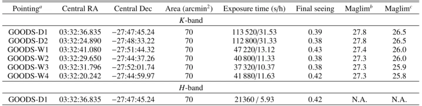
K-band GOODS-D1 03:32:36.835 −27:47:45.24 70 113 520/31.53 0.39 27.8 26.5 GOODS-D2 03:32:24.890 −27:48:33.22 70 112 800/31.33 0.38 27.8 26.5 GOODS-W1 03:32:41.080 −27:51:44.32 70 47 220/13.12 0.43 27.4 26.0 GOODS-W2 03:32:29.650 −27:44:37.26 70 40 800/11.33 0.38 27.3 26.0 GOODS-W3 03:32:31.796 −27:52:01.74 70 37 320/10.37 0.38 27.3 25.9 GOODS-W4 03:32:20.242 −27:44:59.97 70 41 880/11.63 0.42 27.3 25.8 H-band
GOODS-D1 03:32:36.835 −27:47:45.24 70 21360/ 5.93 0.42 N.A. N.A. Notes.(a)Each pointing has been rotated to PA= −19.5 deg.(b)At 1σ arcsec−2.(c)At 5σ in 1 FWHM.
This image currently provides a unique combination of depth and area in the K-band.
During the earliest observations, several frames were ac-quired in the H and Br-γ filters, over the GD1 pointing. They were taken accidently due to a temporarily miscalibration of the Hawk-I filter wheel. We have also reduced these images, and make them available, although they have not been calibrated nor used in any scientific analysis.
Table2 summarises the location and exposure time of the various pointings.
3. Data acquisition and reduction
3.1. Observations
All imaging in the K-band was obtained with individual images of 10 s of integration, averaged in sets of 12 images during ac-quisition (in ESO jargon these two parameters are referred to as DIT and NDIT, respectively). In the case of the Y-band images we adopted DIT= 30 and NDIT = 4. A random dithering pat-tern with a typical offset of 12 arcsec was applied in all cases. Observations were scheduled in Observing Blocks of about 1 hr of execution each, corresponding to about 45 and 48 min of exposure in K and Y, respectively. The position angle of each Observing Block (OB) was rotated by 90 degrees, so that the fi-nal mosaics are the results of individual images obtained with
different physical regions of the detectors (which allowed us to test the accuracy of the photometric and calibration procedures). All observations were executed in Service Mode, over a se-ries of ESO observing periods from P86 to P90. We retrieved from the archive all the images obtained during these runs, in-cluding those that were not graded within specifications during the observations. All these images were then analysed with an automated pipeline to assess their quality. We have included in the final coadded frames also some of the images graded “out of specs”, but have excluded those with wildly-discrepant seeing, poor photometric quality or other cosmetic defects. For this rea-son the actual exposure times listed in Tables1and2are slightly different from pointing to pointing, even though we originally planned identical exposure times.
3.2. Data reduction
We initially used two pipelines to independently reduce the im-ages acquired in the first year of observations. One pipeline has been developed at the Rome Observatory, and is derived from a pipeline used to reduce LBT imaging data both in the visible and in the infrared. In its former version it was used to reduce the earliest Hawk-I data in GOODS-S (Castellano
et al. 2010a,b). The second pipeline has been developed at the
University of Edinburgh (originally to reduce UKIRT WFCAM and Gemini NIRI data;Targett et al. 2011). We then compared the two pipelines and the resulting reduced images, both in terms
of conceptual steps and algorithms adopted, as well as in terms of the final image mosaic. The two results agreed very well and this comparison was utilised to help yield a final, optimised version of the Rome pipeline. This refined Rome pipeline has been used in the final processing of all the data, including a re-processing of any previously-reduced images. For this reason the images produced here are slightly different/better than those used inCastellano et al.(2010b). The final reduction pipeline is described in more detail in a separate paper (Paris et al., in prep.) but we describe here the basic steps (that follow the usual recipe of infrared imaging data reduction) and specific features.
3.2.1. Pre-reduction
The raw images were retrieved from the ESO archive and each Observing Block was processed separately at this stage. The initial reduction procedure consists of the removal of the dark current and application of a flat-field in order to normalise the response of each image pixel. Each flat-field is obtained from twilight sky-flats obtained in the same day of the observations, or in the day immediately before or after when not available. Typically between 30 and 60 images are used to compute the flat-field. At first each scientific frame is subtracted by a median stack dark image obtained by combining a set of dark frames with the same EXPTIME and NDIT values of the observation set images. Then a median stack flat image (masterflat) is cre-ated, by combining a set of sky flats taken with the same filter as the observation set, each subtracted by its own dark. While com-bining, each flat is normalised by its own median background level, in order to obtain a final median stack flat normalised to unity. Each scientific image is then divided by the masterflat, so the response of pixels is finally homogenised. During this pre-reduction stage pixel masks are also created to flag saturated regions, cosmic ray events, satellite tracks and bad (hot/cold) pixels. We have also developed a specific procedure to take the effects of persistence into account – i.e. the residual counts left by bright objects on the subsequent images. After some tests, we decided to identify all the pixels that are above 104counts in a given image and mask them out from the following image. Given the large number of subsequent images, this efficiently masks out most of the pixels affected by persistence. We assume that the remaining contribution is efficiently wiped out by the dithering process, such that it does not yield detectable sources. We also note that no correction has been applied for non-linearity: the individual exposures are below the threshold for non-linearity effects, and only few, very bright sources are detected in individ-ual exposres, the others being within the background noise. We therefore expects that some residual non-linearity may at most affect only the brightest sources that are not the scientific target of the survey.
3.2.2. Background subtraction
After pre-reduction, the image backgrounds are still far from flat. Structures appear both at small and at large scales due to a vari-ety of causes, such as pupil ghosts, dust, and sky-background variation during the observation (which is particularly strong in the near-infrared, especially in K). We have developed spe-cialised algorithms to carefully remove these structures. Since they are assumed to be additive features, the basic operation is to create and then subtract maps of the background from each image. The first map is a sigma-clipped median-stacked image of the observations included in a temporal window – typically
-0.4 -0.2 0 0.2 0.4 1000
-0.5 0 0.5
Fig. 3.Differences in RA and Dec for all the objects detected in the overlapping region between the GD1 and GD2 pointings. The two insets on the right and top show the resulting distributions.
of about 10 minutes – around the processed image. Y-band im-ages show a substantial improvement after just the subtraction of this first sky background map, while a further large-scale poly-nomial fit to the residual features has been further subtracted from the K-band images. At the end of this stage, in which each Observing Block has been processed separately, images are flat and ready to be processed to create the final mosaic.
3.2.3. Astrometric solution
In order to perform the coaddition, an accurate astrometric cal-ibration has to be performed. In fact images show geometrical distortions arising from the positional errors of each pixel due to many causes, such as optical distortions, atmospheric refrac-tion, rotation of chips, non-integer dithering pattern, etc. The procedure of astrometric calibration consists of two basic opera-tions: the correction of relative linear offsets between exposures and the refined absolute global calibration. For each exposure, a S
(Bertin & Arnouts 1996) catalogue is created, and the relative linear calibration between exposures is achieved by correcting for the offsets between source coordinates, com-puted by the cross-matching with a catalogue chosen as refer-ence. The absolute calibration is done by providing an absolute reference catalogue and correcting for distortions through the cross-matching of source coordinates and by storing the final corrected solution into the header of the images. We use as ref-erence images the CANDELS WFC3/IR images (Galametz et al.2013;Guo et al. 2013) for both the UDS and GOODS-S fields.
This approach was applied to each individual image separately. The final accuracy of the astrometric solution has been tested using the regions with overlapping images. As an example, we show in Fig.3the distribution of the differences in RA and Dec for the objects that fall in the large overlapping area between the GD1 and GD2 pointings. The analysis is done on 3815 matched sources, and the resulting root-mean squares (rms) are σRA = 0.06700and σ
3.2.4. Estimate of absolute noise image
Absolute noise maps for each exposure are created directly from the raw images. They are based on the assumption that the noise is given by the Poisson statistics of the counts detected in each pixel of the original frames. This contribution is propagated to take the scaling applied to each pixel during processing (includ-ing flat-field(includ-ing, normalization of exposure times rescal(includ-ing of zero-points etc) into account. The resulting absolute noise map at pixel X, Y, σ(X, Y)ican be obtained by the following formula:
σ(X, Y)i= s RAW(X, Y)i gaini × 1.0 √ FLAT(X, Y)i × √1.0 ndit (1)
where i= 1, 2, 3, 4 is an index that represents the number of the chip of HAWK-I, RAW(X, Y)i the raw number counts at pixel X, Y, gainiis the read-out gain, FLAT(X, Y)iis the value of the flat-field image used to calibrate the raw image, and ndit is the value of NDIT.
3.2.5. Coaddition
Our pipeline uses SWarp (Bertin et al. 2002) to resample all the processed images, implementing it into a procedure designed to properly propagate the absolute rms obtained as above. At first a global header is created from the input images that are re-sampled according to the geometry described in the resulting global header. In order to obtain a physical exposure and an rms map of the final mosaic, during the resampling the inter-nal WEIGHT_TYPE parameter has to be set to the MAP_rms modality, so that a noise map has to be given for each expo-sure. During the resampling stage, images with bad astromet-ric information are rejected, while for each resampled image SWarp provides a weight map in output. The last step is to per-form a weighted summation of all the resampled images, us-ing as weight wi(X, Y) = 1/σi(X, Y)2, where σ for each pixel is given by Eq. (1). The final rms map is obtained simply by: rms(X, Y) = 1/
q Pn
i=1w(X, Y)
i. These rms images are released along with the science data (see below). Since the current ver-sion of SWarp is not able to produce these rms images, these steps have been obtained with a specific pipeline.
3.2.6. Photometric calibration
At the end of each reduction we have adopted a careful pro-cedure to calibrate the photometry and estimate the zero point, independently for each pointing. For each pointing we have cho-sen at least one OB qualified as photometric during the obser-vations, and we have stacked them in order to obtain a mosaic of the field with '1 h of exposure, in good photometric condi-tions and with consistent airmass. We then retrieved from the ESO archive a set of standard stars observed at the same air-mass as the scientific images, and as close as possible in time to the observations. We have reduced the standards using the same calibration frames used for the scientific images. At the end of the reduction we have extracted a catalogue for each standard calibration image and by comparing the magnitude of the stan-dard star, corrected for extinction, with the magnitude reported in the literature, we have obtained a first estimate of the zero point zp1 that we assume can be straight-forwardly applied to the stacked OB described above. Finally, we have extracted and cross-matched two catalogues, the first from the full complete
mosaic, and the second from the 1-h mosaic, calibrated with zp1. By comparing the differences in magnitude between the sources in the two catalogues we have achieved a final refined estimate of the zero-point. To minimise possible systematic offsets all these operations have been executed using the MAG_BEST magni-tude obtained by SExtractor on the brightest objects only. We estimate that the typical uncertainty in the derivation of the ze-ropoints is of ±0.02 mag, as obtained from repeated estimate of the ZP on independent sets of OBs and standards of the same pointing.
4. Validation and tests on photometry
We have performed a number of tests, both on intermediate steps of data reduction as well as on the final images, comparing them with external data sets.
We report here two classes of comparisons that may be of general interest for the reader. In all these cases we have ob-tained single-band photometric catalogues using SExtractor and cross-matched the catalogues using the measured RA and Dec. We then use the difference in observed total magnitudes for the objects in common between the various catalogues. We note that the stability of the photometric solution is in general quite good, to the extent that its validation has been ultimately limited by the uncertainties in the photometry. As our fields are relatively devoid of stars, most of the objects that we have used for com-parisons are galaxies. It is well known that, when galaxies are observed with different seeing, sampling and depth, the estimate of their total magnitude is affected by systematics that depend on the size, profile and surface brightness of individual objects. To minimise these effects we have performed these tests on bright objects (typically those detected at S/N > 35) and used Kron magnitudes, as measured by SExtractor, that are relatively less sensitive to these effects.
First, we compared the catalogues obtained from fully-reduced stacks of the different pointings in the overlapping re-gions. They have revealed small differences (usually within the errors) of the zeropoints that have been averaged out in order to provide an internally-consistent data set.
All the pointings of our survey have overlapping regions with (at least one) nearby pointing. The typical size of these overlap-ping areas is 0.500 × 70 in UDS, and larger in GOODS-S (see Fig.2). We have used the observed systematic offsets between the magnitudes in the various pointings (as shown in Fig.4) as a measure of the systematic differences in the derived zeropoints. As shown in Fig.4, these offsets are always small (of the order of 0.01–0.02 mag), consistent with the uncertainty of the flux calibration. For the UDS, we have tied the photometry to the zeropoint of UDS2, i.e. we have renormalised the original ze-ropoints of UDS1 and UDS3 in order to make the photometry of the overlapping areas fully consistent. In GOODS-S we have similarly tied the photometry to that derived from GD1.
We have also compared our final images to the previously available images obtained by wider-field imagers. The goal of this exercise is to further check against large-scale trends that may be left in our data, that cannot be identified on the overlap-ping areas.
For the UDS we have used the DR8 release of the UKIDSS Deep Survey, that has imaged a 0.77 deg2field that includes the CANDELS field. For the GOODS-S we use the output of the Extended Chandra Deep Field (ECDFS), that was obtained with the SOFI instrument on NTT. Results are shown in Figs.5and6. Again, they show no major systematic trends in the data.
0 1000 2000 -1 -0.5 0 0.5 1 x avg=-0.006 -2000 -1000 0 1000 2000 -1 -0.5 0 0.5 1 y avg=-0.006
Fig. 4.Difference in magnitude for objects detected in both the GD1 and GD2 fields, as a function of the X, Y position in pixels in the GD2 field. Since the field is rotated by −19.5 degrees, using RA and Dec could hide real trends in the reduced data. This plot is before any renormalization of the zeropoint (see text for details).
34.25 34.3 34.35 -1 -0.5 0 0.5 1 Right Ascension offset=0.011 UDS2 vs. DR8-UDS -5.25 -5.2 -5.15 -1 -0.5 0 0.5 1 Declination offset=0.011
Fig. 5.Difference in magnitude for objects detected in the UDS2 point-ing and in the UKIDSS DR8 release, as a function of RA and Dec (see text for details).
5. Data release
Both images and catalogues derived from the HUGS data are made publicly available. They can be retrieved from the ASTRODEEP website2as well as from the ESO, HST, and CDS
archives. 5.1. Images
We have finally obtained a set of mosaics of each data set, that we make publicly available. For each data set we release:
– The coadded image for each pointing (UDS1,2,3, GOODS-D1, D2, W1, W2, W3 and W4) – these are all calibrated and rescaled to a standard zeropoint of 27.5 for the K-band images, and 27.0 for the Y-band;
2 http://www.astrodeep.eu/HUGS -2000 -1000 0 1000 2000 -1 -0.5 0 0.5 1 x avg=-0.012 -2000 -1000 0 1000 2000 -1 -0.5 0 0.5 1 y avg=-0.012
Fig. 6.As in Fig.5, for the GD2 and ECDFS field. As in Fig.4we plot the difference as a function of the X, Y position in pixels in the GD2 field. Since the field is rotated by −19.5 degrees, using RA and Dec could hide real trends in the reduced data (see text for further details).
– The relevant absolute rms images, with the same flux scale; – A global mosaic of the two fields in each band, with the
rele-vant absolute rms, after homogenizing all images to the same PSF. This has been done by degrading the highest quality im-ages to the one with the poorest seeing. Although the seeing is fairly constant and of excellent quality, this procedure in-evitably degrades some of the information contained in the data. The correlation of the background pixels is also visibly different across each image, because of the different degree of filtering applied to each original pointing.
– A global mosaic of the two fields in each band, with the rel-evant absolute rms, without any correction for the different PSFs. These mosaics have varying PSF across the fields (in a smooth way across the overlapping region) but do not show a varying degree of correlation in the background. These are probably most useful for illustrative purposes, and have been used in the subsequent illustrations.
We remark that the most accurate scientific analysis is, for most application, obtained by separately using the individual point-ings and then combining the output in an appropriate way, as we did for the derivation of the multi-colour catalogues in the UDS (Galametz et al 2013, and see below).
The final images for the two fields are shown in Figs.7and8. The images shown are those obtained by combining the vari-ous pointings into a single mosaic, without performing any PSF matching prior to coaddition.
Figures7and8also show the rms images of the final mo-saics. The relics of cosmetic defects are clearly visible in the rms images, as are less exposed regions where some of the data have been removed to eliminate defects or trails.
The comparison between the depth of the HUGS images and the CANDELS H-band images is performed more thoroughly in the next section using the multi-wavelength catalogues. In the meantime, a visual comparison is offered in Fig.9, where we compare the deepest region from HUGS and CANDELS. It can be immediately appreciated that the depth and quality of the HUGS images is comparable in all aspects to the WFC3 data.
Because of the inhomogeneous depth of the final mosaics, the limiting magnitude is not constant across the fields, in partic-ular for the GOODS-S imaging. This is shown in Fig.10, where
Fig. 7.Top: final image of the UDS field in the Y band. Bottom: weight image, computed as described in the text. The bottom scale represents the rms, normalised to its peak value. Darker regions have lower rms, or equivalently higher relative weight, and hence correspond to deeper regions of the images. The left-most pointing (UDS3) is slightly shallower than the other two pointings, despite the fact they have the same exposure time, because the average background observed during the observations turned out to be larger than for the other two pointings.
Fig. 8.Left: final image on the GOODS-South field, in the K band. Right: weight image, computed as described in the text. Darker regions have higher weight – hence correspond to deeper regions of the images.
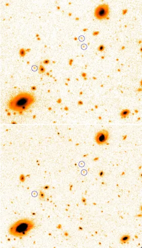
Fig. 9.Centre of the GOODS-S field as observed with Hawk-I in the K-band (upper) and with WFC3/IR in the H-band (bottom). The dis-played area is 1 arcmin wide, and is extracted from the region where the Hawk-I data have the maximum depth. The H-band image is from the CANDELS Deep area. Both images have a dynamic range extending from 0.5σ to 100σ per pixel, on a logarithmic scale. Objects encircled have H160' 26 and a colour H − K ' 0.5, typical of faint galaxies.
we plot the distribution of the magnitude limit in the two fields. This has been computed converting the calibrated rms contained in each pixel into a 1σ magnitude limit in 1 arcsec2. The two peaks in the UDS field come from the slightly shallow exposure obtained in the UDS3 pointing, where the sky background ef-fectively observed in the data was higher than the average in the other two. In GOODS-S, the 4 broad peaks in the distribution of the magnitude limits come from the complex geometry of the exposure, as shown in Fig.8.
5.2. Catalogues
Catalogues from the HUGS images can be extracted in two dif-ferent ways, either as “single band”, i.e. using the HUGS images as detection image, or adding them to the full multi-wavelength suite of data in CANDELS.
5.2.1. Single band catalogues
Single-band catalogues are, in principle, straightforward to ob-tain. We have used the SExtractor code to obtain single-band detected catalogues that are distributed along with the images. However, a compromise must be achieved in this case between two conflicting requirements. First, to make full use of the
Fig. 10.Distributions of limiting magnitude in the 3 HUGS images, as described in the legend. The lower x-axis shows the limiting magnitude computed at 1σ in an area of 1 arcsec2, the upper at 5σ in an area of
0.4 arcsec2, comparable to the average FWHM. Note that the latter is not
the total magnitude of objects detected at 5σ in an area of 0.4 arcsec2,
since no aperture correction has been applied.
largest possible depth, the detection should be made on the global mosaic, especially in GOODS where the overlaps be-tween the various pointings are significant. However, since the detection process must be tuned to the PSF of the images, and given the different seeing within the HUGS images, to obtain a fully-consistent catalogue we have used as input images the seeing-homogenised images presented above. This somewhat limits the possibility of detecting the faintest galaxies in the pointings with the best seeing, although the seeing variation among the various images is not dramatic (see Tables1and2). We deemed this procedure as the most appropriate to obtain single-band catalogues, that are made publicly available for fu-ture use. For the same reason, the number counts presented in the next section have been obtained with a slightly different pro-cedure that we describe in the next section. Summarizing, the two public catalogues that we derive have been obtained using SExtractor on the seeing-averaged mosaics of both the UDS and GOODS-S HUGS imaging. We have applied a smoothing be-fore detection (of the same size of the PSF), and used a minimal detection area of 9 pixels, requiring S/N > 3 in such an area.
5.2.2. Multi-wavelength catalogues
We have included the photometry extracted from the HUGS images (both in K and in Y) in the UDS and GOODS multi-wavelength catalogues described inGalametz et al.(2013) and
Guo et al.(2013) respectively. In both cases we have detected
the objects in the WFC3 H-band image from CANDELS, and performed PSF-matched photometry on the HUGS images. This has been accomplished by using the TFIT package (Laidler et al. 2007) to properly take the morphology of each object into ac-count during the deblending process. We refer the reader to those two papers for more details. The Guo et al. catalogue
Fig. 11.Fractions of objects in the CANDELS catalogues that have a detected flux in the HUGS data, as a function of the H-band magnitude. Here the H-band is measured on the CANDELS F160W images, and the corresponding K-band flux is measured with the TFIT code on the final HUGS images. Results are shown for two different signal-to-noise ratios in the K-band, and for the two HUGS fields (as shown in the legends). Errors are computed assuming simple Poisson statistics.
was compiled using only the first epoch of Hawk-I images in GOODS-S. We have therefore re-extracted the K-band photom-etry using the final images described here, for all the objects detected in the H-band. This catalogue is released here.
We note that, to deal with the different PSFs of the vari-ous images, we have independently processed each of the fi-nal individual pointings described above, and thereafter weight-averaged the photometry of objects detected on multiple images to obtain the final photometry. Clearly, following this proce-dure, the ultimate depth of the catalogue is driven by the WFC3 H-band image. It may be of some interest to show how e ffec-tive the HUGS images are in providing us with useful infor-mation on the CANDELS-detected objects, since that is one of the main aims of the HUGS survey. This is shown in Fig. 11, where we plot the fraction of objects that are detected at 5σ or 1σ in the K-band as a function of the H-band magnitude. In the case of GOODS-S, it is seen that as many as 90% of the H-detected galaxies have some flux measured at S/N > 1 in the K-band, down to the faintest limits of the H-band catalogue, and that nearly 60% of the H ' 26 galaxies (and 15% of the H ' 27 galaxies) have a solid K-band detection with S/N > 5. We note that these statistics are measured on the full GOODS-S HUGS area, which is highly inhomogeneous in depth both in the Hand K bands. This result confirms that our original goal has been achieved, and in particular that our pointing strategy has been quite efficient in covering the inhomogeneous GOODS-S field at the required depth.
6. Number counts
Finally, we have derived the number counts in the K-band, com-bining both UDS and GOODS-S images. At variance with the
procedure described above, we decided not to use the seeing-homogeneised mosaics since their use would limit the final depth of the catalogues (due to the compromised seeing). Within the UDS field we therefore extracted independent catalogues from each of the three UDS Hawk-I pointings (which have notably different seeing), optimizing each catalogue to the relevant PSF. In the case of GOODS-S, we built a specific mosaic using the two deep pointings D1 and D2 as well as W2 and W3. These four pointings have remarkably similar seeing, thus enabling us to build a mosaic without any additional seeing-homogenization, which allows us to exploit the deepest images obtained in HUGS without degrading their quality.
Four catalogues (UDS1, UDS2, UDS3, GOODS-D1+D2+W2+W3) have thus been obtained using SExtractor, as described above. As already mentioned we use the Kron magnitudes (termed MAG_AUTO in SExtractor), and the systematic errors associated with their use are corrected with the simulations that we describe below. Number counts have been derived independently from each image using the procedure described below, and a weighted average of these has then been used to obtain the final number counts. The small overlap between the UDS fields means that these three catalogues are not entirely independent, but we have ignored this effect since the objects detected in more than one image represent only '1% of the total sample. After trimming the outer regions of the images, the final area over which we compute the number counts is 340.58 square arcmin, i.e. about 1/10th of a square degree. We note however that the area over which the number counts are measured is in practice a function of magnitude because of the inhomogeneity of our exposure maps, As a result, the deepest number counts (i.e. those determined at K > 25) are in practice determined from a sub-area of 50.17 square arcmin within the GOODS-S field.
Central to a robust determination of the number counts is a thorough and reliable estimate of the incompleteness and other systematics/biases, which must be obtained through the use of simulations. As is now standard procedure, we have performed these simulations by inserting fake objects into the real images with a range of magnitudes (from K= 18 to K = 27.5) and sizes (we used exponential profiles with observed half-light radius chosen randomly from within the range 0–0.4 arcsec). These ob-jects have also been convolved with the observed PSF before being placed at random positions in the field, including areas where known objects are already detected. Object detection is therefore achieved in the very same way as for the real objects in the original images, and the output magnitudes measured for the fake objects (when detected) are measured, along with the de-tected fraction. Only 200 objects have been placed in each run, in order to minimise excessive and unrealistic crowding effects. Simulations have been repeated until 106objects have been sim-ulated in each field.
To use these simulations, we have followed exactly the same approach used in the analysis of the deepest K-band image obtained so far, in the AO-assisted Subaru Super Deep Field (SSDF,Minowa et al. 2005; the technique is similar to the one adopted also by previous analysis, e.g.Smail et al. 1995). This method takes into account three sources of systematic error. The first is the incompleteness, i.e. the fraction of objects lost as a function of their real input magnitude. The second is the system-atic bias that can arise in the estimate of total magnitude due to surface brightness sensitivity. Specifically, at low signal-to-noise ratios (S/N), the Kron magnitudes that we use (MAG_AUTO in SExtractor) progressively underestimate the real magnitudes of the detected galaxies; our simulations indicate that at faint
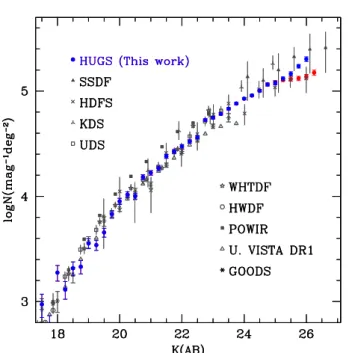
Fig. 12.Number counts in the K-band, from HUGS and from the recent literature (see text for full references for the previous surveys). In blue are the HUGS counts corrected for incompleteness assuming a faint galaxy size distribution spanning the range rhl= 0.1–0.3 arcsec. In red
we show the counts that are derived assuming point-like sources. Recent results from the literature are also shown: SSDF:Minowa et al.(2005), HDFS: Labbé et al. (2003), KDS: Moustakas et al. (1997), UDS: Cirasuolo et al. (2010), WHTDF:Cristóbal-Hornillos et al. (2003), HWDF:Huang et al.(1997), POWIR:Conselice et al.(2008), U.VISTA DR1:McCracken et al.(2012), GOODS:Grazian et al.(2006).
fluxes this effect can easily be 0.1–0.15 mag, and neglecting it would bias the estimate of the slope of the number counts. Finally, there is the effect of flux-boosting; fainter sources can be promoted to brighter magnitudes (hence contaminating the number counts) when they happen to fall on a positive noise fluctuation. Technically, this is done by first extracting from the simulations the transfer matrix Toi that gives the fraction of galaxies with input magnitude mi that are detected with out-put magnitude mo. We then build the probability matrix Piothat gives the probability that an artificial object detected with mi ac-tually has a magnitude mo. The elements of Pioare computed as Pio= Toini/ PkToknk, where niis the number of artificial objects with magnitude mi. In building this matrix the relative fraction of input galaxies must scale with a realistic slope, in order to appropriately weight the number of galaxies close to or fainter than the magnitude limit. To ensure this is done properly, ob-jects are simulated up to K ' 27.5, much deeper than the formal 5-σ detection limit of even the deepest regions of our Hawk-I imaging. This is done assuming the true intrinsic number counts follow a power-law whose slope is varied until a consistent result is achieved with the recovered number counts. The final number counts are finally computed as ncori = PoPion
gal
o , where n gal o are the raw (observed) number counts. We defer toMinowa et al.
(2005) for more details.
The estimate of the size and magnitude dependence of the correction depends on a critical assumption, namely the distri-bution of galaxy sizes. At the exquisite resolution of the HUGS images the difference between compact and point-like sources is measurable, as in theMinowa et al.(2005) data. To get an esti-mate of the real size distribution of the galaxies at faint K-band magnitudes, we have looked at the half-light radius (rhl) of galaxies as measured by SExtractor in the H-band WFC3 images
Table 3. K-band galaxy number counts derived from the HUGS survey, corrected for incompleteness and other systematic effects as described in the text.
Magnitude bin log (N)a log (σ(N))a log (N)b log (σ(N))b
24.00 4.9274 3.2965 4.9283 3.2969 24.25 4.9582 3.3285 4.9588 3.3288 24.50 5.0033 3.4016 5.0021 3.4010 24.75 5.0639 3.5820 5.0619 3.5810 25.00 5.0827 3.6783 5.0774 3.6757 25.25 5.1068 3.6904 5.1187 3.6964 25.50 5.1147 3.7863 5.1648 3.8114 25.75 5.1203 3.7891 5.2363 3.8471 26.00 5.1391 3.7985 5.3038 4.0063 26.25 5.1758 3.9423 – –
Notes. Number densities are in units of galaxies per magnitude per square degree. The full table is available at the CDS and athttp:// www.oa-roma.inaf.it/HUGS. (a) Assuming unresolved
morpholo-gies for galaxies; see text for details.(b) Assuming a distributions of
galaxy half-light radius from 0.1 arcsec to 0.3 arcsec; see text for details.
in CANDELS-GOODS. While the rhlof stars is 0.15 arcsec (cor-responding to the angular resolution limit of H-band HST imag-ing), we find that galaxies at K ' 26 (the typical magnitude where incompleteness is effective in the deepest GOODS data, see below) have rhltypically in the range 0.15–0.3 arcsec. There is also a clear trend with magnitude, with brighter galaxies being even larger than 0.3 arcsec, while the typical rhl for galaxies at K ' 27 appears to be much closer to 0.15 arcsec (the value in-dicative of unresolved objects). We therefore computed the cor-rection for incompleteness in two cases: i) assuming point-like sources (as inMinowa et al. 2005) and ii) assuming a distribution in size between 0.1 and 0.3 arcsec. We performed this exercise independently in the various images for both fields and then av-eraged the resulting number counts, weighting them by the area of the appropriate parent image. Finally, to minimise the sen-sitivity of our derived number counts to these corrections, we have used the counts from the various images only when the in-completeness is negligible (<5%), the only exception being the deepest areas in GOODS-S where we have of course used our best estimate of the appropriate corrections to push our derived number counts to the faintest limits.
The derived number counts are given in Table3. They are also shown in Fig.12, for both assumptions about galaxy size, compared with a number of recent results from the literature (SSDF:Minowa et al. 2005, HDFS:Labbé et al. 2003, KDS:
Moustakas et al. 1997, UDS: Cirasuolo et al. 2010, WHTDF:
Cristóbal-Hornillos et al. 2003, HWDF: Huang et al. 1997,
POWIR:Conselice et al. 2008, U.VISTA DR1:McCracken et al. 2012, GOODS:Grazian et al. 2006). Uncertainties have been es-timated assuming simple Poisson errors.
As expected, the number counts agree very well with pre-vious results from the literature. It is immediately appreciated that the HUGS number counts exceed in depth and statistical ac-curacy all previous estimates at the faint magnitudes, the only exception being the very faintest bin plotted from the SSDF. The latter used AO-assisted observations to achieve a very small PSF (0.18 arcsec), making these observations more sensitive than HUGS to the detection of very faint point-like sources. The faint counts from SSDF are, however, very uncertain, although we note that they are consistent with the HUGS counts derived as-suming extended galaxy morphology.
At the faint limit, it is immediately clear how dramatic the impact of the assumptions on galaxy size is. Assuming point-like sources we confirm the flattening of the number counts at K ' 24–26 reported by Minowa et al. (2005), with a slope dlog N/dm of about 0.15, in our case with a much larger statisti-cal accuracy (due to the 50× larger field of view of our images). However, assuming instead a typical galaxy size in the range 0.1–0.3 arcsec, we find that the slope of the number counts re-mains essentially unchanged up to K ' 26, with a slope of about 0.18.
This difference in slope is potentially very important for es-tablishing the contribution of detected galaxies to the extragalac-tic background light (EBL). As noted byMinowa et al.(2005), a relatively shallow slope at faint limits (as found assuming point-like sources) would lead to a major discrepancy with the ob-served EBL, leaving space for additional sources, for instance primeval galaxies. Conversely, if we assume that the steep slope that we find for resolved galaxies holds to even fainter limit, the consequence is that most of the diffuse EBL observed from space can be ascribed to ordinary galaxies, without the need to invoke for more exotic populations.
A robust determination of this effect, however, requires more refined simulation and analysis of the galaxy size distribution as a function of magnitude, possibly including even deeper data such as is provided in the H-band by HUDF12. However, such an analysis is beyond the scope of this current paper.
7. Summary
We have present in this paper the results of a new, ultra-deep, near-infrared imaging survey executed with the Hawk-I imager at the ESO VLT. This survey, named HUGS, provides deep, high-quality imaging in the K and Y bands over the portions of the UKIDSS UDS and GOODS-South fields covered by the CANDELS HST WFC3/IR survey. While the bulk of the data presented here comes from a program specifically designed to cover CANDELS (the ESO Large Program 186.A-0898, P.I. Fontana), we have also included in our analysis other data com-ing from previous observations on GOODS-S, which were ac-quired either during the Science Verification Phase (60.A-9284) or in the framework of another program designed to look for z '7 galaxies (the ESO Large Program 181.A0717, P.I. Fontana,
Castellano et al. 2010a,b). These data comprise nearly all the
available Hawk-I data on GOODS-S and have been homoge-neously reduced, discussed and made publicly available here.
This paper describes the survey strategy, the observational campaign and the data reduction process. For further details on the data reduction we refer the reader to the previous sections, which give full details. We simply mention here that we have followed standard recipes for these images, adopting a num-ber of validation controls. First, we have used two independent pipelines (one developed in Rome and one in Edinburgh) to re-duce the first epoch of data, and cross-compared the results, find-ing excellent consistency and agreement. In addition, we used the large wealth of independent images acquired over each field to internally validate the data. At the end of these tests, we are confident that the observation uncertainties are under control, typically at the level of few percent.
Similarly, full details of the observing strategy and resulting data are described in the text. We refer the reader in particular to the tables and figures for further information. We summarise here the fundamental aspects of our survey.
– HUGS has been designed to complement the CANDELS data in the two fields where crucial infrared data of the nec-essary depth cannot or have not been obtained with WFC3: deep K-band imaging in GOODS-S, and deep Y and K-band imaging in the UDS. The depth has been tuned in order to match the depth of the WFC3 J and H imaging. For instance, the K-band limit is set about 0.5 mag shallower than H160 senstivity limit, in order to match the average H − K colour of faint galaxies.
– Pointings have also been optimised to cover CANDELS. In the UDS, we covered 85% of the CANDELS area with 3 different, marginally-overlapping Hawk-I pointings. For the K-band in GOODS-S we adopted a more complicated pattern, comprising 6 different pointings (two “Deep” and four “Wide”) as described in Fig. 2. This has allowed us to vary the exposure time over the field in order to match the varying depth of the CANDELS images. The Y-band in GOODS-S covers about 60% of the eastern CANDELS area. – In the UDS, the exposure times of each pointing are '13 h in the K-band and '8 h in the Y-band. The seeing is 0.37– 0.43 arcsec in the K-band and 0.45–0.5 arcsec in the Y band. The corresponding limiting magnitudes are mlim(K) ' 26, mlim(Y) ' 26.8 (5σ in one FWHM) or mlim(K) ' 27.3, mlim(Y) ' 28.3 (1σ per arcsec2).
– In GOODS-S, the total exposure time in the K-band (summed over six pointings) is '107 h. Because of the com-plex geometry, this corresponds to an exposure of 60–80 h in the central area (the sub-region covered by CANDELS “Deep”) and 12–20 h over the remainder (the CANDELS “Wide area”). The final average seeing is remarkably good and constant, with 4 pointings with FWHM ' 0.38 arcsec (notably including the two deepest) and 2 pointings with FWHM '0.42 arcsec. On the final stacked images, the lim-iting magnitudes in the deepest area are mlim(K) ' 27. (5σ in one FWHM) or mlim(K) ' 28.3, mlim(Y) ' 28.3 (1σ per arcsec2).
– We have derived from the HUGS images two different types of catalogue – a K-band selected catalogue that we use to estimate number counts, and PSF-matched catalogues for all the H-selected galaxies detected in the CANDELS im-ages. For the UDS, the corresponding catalogue published in Galametz et al. (2013) already uses the full HUGS data. However, the catalogue for GOODS-S obtained and made available here supercedes the catalogue already published in Guo et al. (2013, which used only a preliminary version of the HUGS data, obtained from shallower observations of the central area (pointings D1 and D2) only).
– Our key and crucial goal of effectively matching the CANDELS depth (for most useful analyses) has been achieved, as shown in Fig.11, where it can be seen that a large fraction of even the faintest H-band CANDELS objects are also clearly detected in our HUGS K-band imaging. Finally we have presented the galaxy number counts in the K-band, as obtained after combining the two HUGS fields. We describe the simulations that we have adopted to correct for the incompleteness and flux boosting at the faintest limits, making different assumptions for the size distribution of faint galaxies. We show that our number counts extend to magnitude limits fainter than any previous survey, other than the rather uncertain faint counts achieved with the AO-assisted images of the SSDF field. The latter have a FWHM of 0.18 arcsec and exposure times comparable to our survey, and hence reach fainter limits for un-resolved objects, but over such a small area ('1 square arcmin)
that they are statistically very uncertain. We show that the slope of the number counts over the faintest bins depends sensitively on the assumed distribution of galaxy sizes. It ranges from 0.18, if we assume that galaxies at K > 26 are unresolved, to 0.22, if we assume that such galaxies have a typical distribution of half-light radii spanning the range 0.1–0.3 arcsec, as suggested by a preliminary analysis of the deepest CANDELS images.
We have made all of the final HUGS images and derived catalogues publicly available at the ASTRODEEP website3 as
well as from the ESO archive.
Acknowledgements. This work would not have been possible without the sup-port and dedication of the whole ESO staff. We thank in particular our supsup-port astronomer Monika Petr-Gotzens. We are also grateful to the memory of Alan Moorwood, who was fundamental in motivating the development of the Hawk-I instrument, with which our survey has been undertaken. We also thank the ref-eree, V. Manieri, for his accurate report. A.F. and J.S.D. acknowledge the con-tribution of the EC FP7 SPACE project ASTRODEEP (Ref. No: 312725). J.S.D. also acknowledges the support of the Royal Society via a Wolfson Research Merit Award, and the support of the ERC through an Advanced Grant. D.C.K. and S.M.F. were supported by US NSF grant AST08-08133. V.W. acknowledges support of the ERC through the starting grant SEDmorph. R.J.M. acknowledges ERC funding via the award of a consolidator grant. This work uses data from the following ESO programs: 60.A-9284, 181.A0717, 186.A-0898.
References
Ashby, M. L. N., Willner, S. P., Fazio, G. G., et al. 2013, ApJ, 769, 80 Bertin, E., & Arnouts, S. 1996, A&AS, 117, 393
Bertin, E., Mellier, Y., Radovich, M., et al. 2002, in Astronomical Data Analysis Software and Systems XI, eds. D. A. Bohlender, D. Durand, & T. H. Handley, ASP Conf. Ser., 281, 228
Caputi, K. I., McLure, R. J., Dunlop, J. S., Cirasuolo, M., & Schael, A. M. 2006, MNRAS, 366, 609
Castellano, M., Fontana, A., Boutsia, K., et al. 2010a, A&A, 511, A20 Castellano, M., Fontana, A., Paris, D., et al. 2010b, A&A, 524, A28 Cirasuolo, M., McLure, R. J., Dunlop, J. S., et al. 2010, MNRAS, 401, 1166 Conselice, C. J., Bundy, K., U, V., et al. 2008, MNRAS, 383, 1366 Cowie, L. L., Gardner, J. P., Lilly, S. J., & McLean, I. 1990, ApJ, 360, L1 Cristóbal-Hornillos, D., Balcells, M., Prieto, M., et al. 2003, ApJ, 595, 71 Ellis, R. S. 1997, ARA&A, 35, 389
Ellis, R. S., McLure, R. J., Dunlop, J. S., et al. 2013, ApJ, 763, L7 Elston, R., Rieke, G. H., & Rieke, M. J. 1988, ApJ, 331, L77 Fontana, A., D’Odorico, S., Poli, F., et al. 2000, AJ, 120, 2206 Fontana, A., Salimbeni, S., Grazian, A., et al. 2006, A&A, 459, 745 Galametz, A., Grazian, A., Fontana, A., et al. 2013, ApJS, 206, 10 Grazian, A., Fontana, A., de Santis, C., et al. 2006, A&A, 449, 951 Grazian, A., Fontana, A., Santini, P., et al. 2014, A&A, submitted Grogin, N. A., Kocevski, D. D., Faber, S. M., et al. 2011, ApJS, 197, 35 Guo, Y., Ferguson, H. C., Giavalisco, M., et al. 2013, ApJS, 207, 24 Heidt, J., Appenzeller, I., Gabasch, A., et al. 2003, A&A, 398, 49 Huang, J.-S., Cowie, L. L., Gardner, J. P., et al. 1997, ApJ, 476, 12 Illingworth, G. D., Magee, D., Oesch, P. A., et al. 2013, ApJS, 209, 6 Kissler-Patig, M., Pirard, J.-F., Casali, M., et al. 2008, A&A, 491, 941 Koekemoer, A. M., Faber, S. M., Ferguson, H. C., et al. 2011, ApJS, 197, 36 Koekemoer, A. M., Ellis, R. S., McLure, R. J., et al. 2013, ApJS, 209, 3 Labbé, I., Franx, M., Rudnick, G., et al. 2003, AJ, 125, 1107
Laidler, V. G., Papovich, C., Grogin, N. A., et al. 2007, PASP, 119, 1325 McCracken, H. J., Capak, P., Salvato, M., et al. 2010, ApJ, 708, 202
McCracken, H. J., Milvang-Jensen, B., Dunlop, J., et al. 2012, A&A, 544, A156 Minowa, Y., Kobayashi, N., Yoshii, Y., et al. 2005, ApJ, 629, 29
3 http://www.astrodeep.eu/HUGS
Moustakas, L. A., Davis, M., Graham, J. R., et al. 1997, ApJ, 475, 445 Oke, J. B. 1974, ApJS, 27, 21
Retzlaff, J., Rosati, P., Dickinson, M., et al. 2010, A&A, 511, A50 Sawicki, M., & Thompson, D. 2005, ApJ, 635, 100
Smail, I., Hogg, D. W., Yan, L., & Cohen, J. G. 1995, ApJ, 449, L105 Targett, T. A., Dunlop, J. S., McLure, R. J., et al. 2011, MNRAS, 412, 295 Vanzella, E., Pentericci, L., Fontana, A., et al. 2011, ApJ, 730, L35 Williams, R. E., Blacker, B., Dickinson, M., et al. 1996, AJ, 112, 1335 Williams, R. E., Baum, S., Bergeron, L. E., et al. 2000, AJ, 120, 2735 Windhorst, R. A., Cohen, S. H., Hathi, N. P., et al. 2011, ApJS, 193, 27
1 INAF – Osservatorio Astronomico di Roma – via Frascati 33, Monte
Porzio Catone, 00040 Rome, Italy
e-mail: adriano.fontana@oa-roma.inaf.it
2 Institute for Astronomy, University of Edinburgh, Royal
Observatory, Edinburgh EH9 3HJ, UK
3 Department of Physics and Astronomy, Sonoma State University,
Rohnert Park, CA, USA
4 Max-Planck-Institut für extraterrestrische Physik (MPE),
Giessenbachstrasse 1, 85748 Garching bei Munchen, Germany
5 The School of Physics and Astronomy, University of Nottingham,
Nottingham, UK
6 Kapteyn Astronomical Institute, University of Groningen, PO Box
800, 9700 AV Groningen, The Netherlands
7 Spitzer Science Center, MC 2206, California Institute of
Technology, 1200 East California Boulevard, Pasadena, CA 91125, USA
8 Department of Physics and Astronomy, University of California,
Irvine, CA, USA
9 CEA-Saclay/DSM/DAPNIA/Service d’Astrophysique, 91191
Gif-sur-Yvette, France
10 National Optical Astronomy Observatories, Tucson, AZ, USA 11 UCO/Lick Observatory, Department of Astronomy and
Astrophysics, University of California, Santa Cruz, CA, 95064, USA
12 Harvard-Smithsonian Center for Astrophysics, Cambridge, MA,
USA
13 Space Telescope Science Institute, Baltimore, MD, USA
14 Department of Astronomy, University of Massachusetts, Amherst,
MA, USA
15 Aix Marseille Université, CNRS, LAM (Laboratoire
d’Astrophysique de Marseille) UMR 7326, 13388 Marseille, France
16 INAF – Osservatorio Astronomico di Trieste, Trieste, Italy 17 Max Planck Institute for Astronomy, Konigstuhl 17, 69117
Heidelberg, Germany
18 Osservatorio Astronomico di Padova, 35122 Padova, Italy
19 Minnesota Institute of Astrophysics and School of Physics and
Astronomy, University of Minnesota, Minneapolis, MN, USA
20 Department of Astronomy, Steward Observatory, University of
Arizona, Tucson, AZ, USA
21 INAF Osservatorio Astronomico di Bologna, Bologna, Italy 22 School of Physics and Astronomy, University of St Andrews, North
Haugh, St Andrews, KY16 9SS, UK
23 Department of Physics and Astronomy, University of Missouri,
Columbia, MO, USA
24 INAF-Osservatorio Astrofisico di Arcetri, Largo Enrico Fermi 5,