HAL Id: hal-02495471
https://hal.inria.fr/hal-02495471v2
Preprint submitted on 12 Mar 2020
HAL is a multi-disciplinary open access
archive for the deposit and dissemination of
sci-entific research documents, whether they are
pub-lished or not. The documents may come from
L’archive ouverte pluridisciplinaire HAL, est
destinée au dépôt et à la diffusion de documents
scientifiques de niveau recherche, publiés ou non,
émanant des établissements d’enseignement et de
1-Synchronous Programming of Large Scale,
Multi-Periodic Real-Time Applications with Functional
Degrees of Freedom
Guillaume Iooss, Marc Pouzet, Albert Cohen, Dumitru Potop-Butucaru, Jean
Souyris, Vincent Bregeon, Philippe Baufreton
To cite this version:
Guillaume Iooss, Marc Pouzet, Albert Cohen, Dumitru Potop-Butucaru, Jean Souyris, et al..
1-Synchronous Programming of Large Scale, Multi-Periodic Real-Time Applications with Functional
Degrees of Freedom. 2020. �hal-02495471v2�
1-Synchronous Programming of Large Scale, Multi-Periodic
Real-Time Applications with Functional Degrees of Freedom
Guillaume Iooss
∗∗Marc Pouzet
†Albert Cohen
‡Dumitru Potop-Butucaru
∗Jean Souyris
§§Vincent Bregeon
§Philippe Baufreton
¶March 12, 2020
Abstract
The design and implementation of reactive, hard real-time systems involves modeling and generating efficient code for the integration of harmonic multi-periodic tasks. Such a reactive system can be modeled as a synchronous program orchestrating computations, state machine transitions and communications. In a harmonic multi-periodic integration program, task execution rates are related through integral ratios. This paper aims at providing a scalable way to implement large systems composed of modular, synchronous reactive tasks, and to generate efficient code satisfying real-time constraints.
The paper describes three incremental extensions to the Lustre language and evaluates them on production applications. First, we propose a clock calculus for 1-synchronous clocks, i.e. strictly periodic clocks with a single activation on their period; we show how the compiler can exploit this information to raise the level of abstraction when integrating tasks at the system level. Second, we allow some variables to have unknown phases, extending the clock inference to gather constraints on unknown phases, using a solver for load balancing over multi-periodic real-time schedules, before instantiating this solution to assign clocks to all reactions of the system. Third, we propose temporally underspecified operations, relevant to many discrete control scenarii, for example on variables with low temporal variability; we show how to express this in a composable way, retaining the Kahn semantics of the synchronous program outside these controlled relaxations, and exploiting slack in the computation to relax the constraints of the real-time load-balancing problem.
Keywords: synchronous languages, clock inference, underspecified computation.
1
Introduction
Dataflow synchronous languages (such as Lustre [6], Signal [3] and many others) provide a simple and rigorous model to reason about, to implement and to validate concurrent computations on streams of data and state machines interactions. These computations and reactions are defined by data flow equations and organized according to their associated clock, which encodes their activation condition. Operationally, synchronous clocks are streams of booleans that determine if a computation or reaction has to be performed at a given logical time step. At
∗Inria
†École normale Supérieure, Université Pierre et Marie Curie ‡Google France. Work done as Inria/ENS
§Airbus ¶
compilation time, clocks define a type system to reason about and to generate efficient code. By definition, clocks implement a logical model of time, but they can also be associated with real-time behavior for applications where the temporal aspect is vital.
In the most general setting, clocks define a very abstract type system carrying little information besides the name of the parent clock they derive from, the name of the associated boolean condition, and mutual exclusion with other clocks deriving from the same parent [6]. Many works considered other classes of clocks with richer properties, and used these to improve code generation or to enable more advanced verification schemes. For example, the N-synchronous model [7] considers ultimately periodic clocks and uses these to relax the synchronous composition hypothesis while determining the maximal size of communication buffers implementing such relaxed compositions.
We study the implementation of large real-time applications, with a special focus on avionics applications certified at the highest levels of criticality. In this context, a so-called integration program orchestrates the com-munication and activation of a large number of tasks, implemented as stateful nodes. Both integration program and individual nodes are implemented in a synchronous language. We study the case in which these nodes are scheduled over multiple harmonic periods and are activated only once over each period.
There is a mismatch between what an engineer wishes to specify and what the syntax of a synchronous language requires. In particular, a programmer might not know when a task should be executed compared to another, or how two tasks on different periods should communicate. Forcing the programmer to fix these details might cause him to take a bad decision, which can degrade the program performance or violate a latency property. In this paper, our idea is to let the programmer specify exactly what he has in mind, without forcing him to specify everything but while leaving him enough control if he wish so. The missing implementation details are left to be filled by the compiler, so that he can select the best decisions.
Contribution This paper contains three contributions, corresponding to three consecutive extension to the Lustre language. The first contribution considers a specialization of a Lustre program to harmonic 1-synchronous clocks, which are periodic clocks that activate exactly once during their period. A single program may compose nodes with multiple periodic activation rates, but these periods must be linked through harmonic ratios. This kind of clocks is essential when capturing the integration of real-time systems from individual synchronous nodes: the integration program orchestrates the whole system from the top-level, following harmonic rates. Individual nodes may trigger finer-grained computations and reactions by sub-sampling their parent clocks with arbitrary boolean conditions (i.e., not necessarily periodic). Our formalization abstracts away the heavy administrative code which would be needed to declare and build all such periodic clocks.
However, this extension alone is difficult to use in the context of large applications. Indeed, writing a program with 1-synchronous clocks involves explicit phase computations, scheduling short-period tasks over the hyperpe-riod (i.e., the least common multiplier of all pehyperpe-riods of the program). For the clock inference and verification to succeed on the integration program, one needs (i) to set the phase of all local variables and, (ii) for every temporal operators changing the clock of a program, to specify exactly which data to communicate from a period to another. In other words, with this formalization, the user is required to manually specify the periodic, top-level schedule of the application, which may be very tedious on real-world systems integrating thousands of tasks, and tricky when embedding architectural and system constraints such as real-time load-balancing across phases, parallelism, etc.
To address this challenge, our second contribution offers to partially specify the clock of local variables in a program, by only specifying the period and not the phase. This program does not have a well-defined synchronous semantics but still implements a Kahn network with a well-defined functional semantics. We present a compilation flow to determine the value of the under-specified phases, resulting in a “classical” Lustre program with fully-specified 1-synchronous clocks. This flow is composed of a clock inference algorithm which gathers the constraints
on the unknown phases, a solver which figures out a valid set of phases, and a pass to reinject these phases inside the integration program. We evaluate our approach on a large real-world avionic application. The solver has to pick a single solution out of the many valid solutions. In order to orient this selection, we also consider two optional variants of a load-balancing cost function, in order to balance the computational work across all phases.
To further align with the needs of control automation applications, our third contribution adds underspecified temporal operators, i.e. operators where the control flow is underspecified and is left to the compiler to decide. This is useful when the user does not care about which precise data is operated upon, e.g. in physical measurements with robustness of the temporal variability, as long as some real-time constraints are enforced on the time range of the data being sampled. We can use this extra information to relax the constraints on the phases.
These extensions were integrated in the open-source Heptagon compiler1.
Outline Section 2 introduces some background about synchronous languages. Section 3 presents our 1-synchronous clock language extension and hyperperiod expansion. Section 4 presents the under-specified clock extension and the associated compilation flow. Section 5 considers the underspecified operators and how it impacts the previous compilation flow. We review some related work in Section 6, before concluding in Section 7.
2
Background
In this section, we provide some background knowledge about synchronous languages. In particular, we define a kernel language on top of which we will build our extensions, and explain it through a running example.
Syntax We consider a simplified version of a synchronous language (inspired by [4]):
node ::= node f (lvardecl) returns (lvardecl) var lvardecl let leq tel lvardecl ::= vardecl; lvardecl |
vardecl ::= id : type(:: ck)? ck ::= . | ck on x leq ::= eq | eq; leq eq ::= pat = exp
exp ::= cst | id | op(exp, . . . , exp) | if id then exp else exp | c fby exp | exp when id | exp whenot id | merge id exp exp
To illustrate this syntax, an example of synchronous program is presented in Figure 1.
For each tick of his clock, the node dummy reads from a variable i and writes to a variable o. These variables produces (resp. consumes) one new integral data per tick of the clock of the node. In order to compute the value of o for a given tick, we declare 2 local variables: half which is a boolean variable on the base clock (.), and temp which is an integer whose clock is . on half, i.e., which is present only when the value of the variable half is true.
The local variable half is computed by the first equation: its value at the very first tick is true, then it is the value of false fby half from the previous tick. The value of this latter expression is false at the first tick, then the value of half from the previous tick. So, the two first values of half are true, then false, then the value of itself 2 ticks in the past. Therefore, half’s value is true for all even ticks, and false for all odd ticks.
node dummy(i : int) returns (o : int) var
half :: bool : .;
temp :: int : . on half; let
half = true fby false fby half; temp = multiply(2, i when half);
o = merge half temp ((0 fby o) whenot half); tel
Figure 1: Example of synchronous program.
The local variable temp is computed by the second equation: its value is twice the value of i. Because i is always present and temp is only present during the even ticks, we need to subsample i to keep only the values from the even ticks (i when half).
Finally, the output variable o is computed by the third equation. Because o is present more often than temp, we need to oversample temp by distinguishing the cases when temp is present or not. Its value is either the value of temp when it is there (half=true), or its previous value (0 fby o) when it is not there (half=false).
Clocks and periodicity In a general Lustre program, a clock can be either the base clock (.), or a sub-clock of another clock (ck on x), according to a sampling defined by a boolean variable x. The clocking analysis associates a clock to every sub-expression, and ensure that they match on both side of an equation, or on all the argument of a function. We can accelerate (resp. decelerate) the clock of an expression by using the operator when (resp. merge).
Notice that in general, this boolean variable can have values which cannot be known statically (if it is an input). However, this is not the case in our example: we have built the variable half to define a clock which activates once every 2 ticks. Its values form a pattern which repeat itself indefinitely, with a period of 2. Because of this repetition, we says that the clock . on half is periodic, and we note its activation value (10). Likewise, we can note the value of half as (T F), where T is true and F is false.
This notation is coming from the N-synchronous model [7, 15, 17]. In general, infinite binary words (w := 0w|1w) can be used to describe the behavior of a clock, where a 1 corresponds to an activation of the clock. An ultimately periodic binary word u(v), where u and v are two finite binary words, is a word built of a prefix u before infinitely repeating v. An ultimately periodic clock is a clock associated to a ultimately periodic binary word. In this paper, we will only consider periodic clocks (v), which are clocks associated to a periodic binary word, i.e. an ultimately periodic binary word with no prefix.
In our example, we had to build half from an equation to define the clock. This becomes quickly heavy in a program with multiple harmonic periods and this is part of the thing we wish to automatize in the rest of this paper. The current operator In our example, we produce o by oversampling temp and by using the merge and the fby operators. As a syntactic sugar, we introduce an operator current(x, c, exp) which oversamples exp according to the boolean variable x, with the initial value c. This initial value is only used if x is false at its first tick.
During compilation, we can remove the current expression by substituting it with a fresh variable v, itself defined by a new equation as a merge expression. The substitution is:
Semantics We consider two semantics for synchronous programs. The first one is the Kahn semantic [10], which keeps track of the sequence of values produced by any flow. Any timing aspect (when this value is produced) is ignored. The second alternative is the dataflow semantics [18, 12], for which both the values and the tick when these values are produced are considered. The later semantic is more strict than the first one.
3
1-synchronous clocks
This section presents our first extension of the Lustre language, which introduces constructs for 1-synchronous clocks.
3.1
1-synchronous clocks and language extension
Definition 1. A 1-synchronous clock is a strictly periodic clock with only one activation per period. This means that a 1-synchronous clock is of the form(0k10n−k−1) (or alternatively 0k(10n−1)), where 0 ≤ k < n; n is called the period and k the phase.
We create a special kind of node, called model node, in which the clock calculus is restricted to 1-synchronous clocks using harmonic periods (i.e., periods which are integral multiple of another). Even if the expressiveness power is reduced on these nodes, this is enough to express integration programs at the top level of real-time system design and implementation. Notice that a model node can use other sub-nodes, corresponding to tasks of the system and which may still use more general Lustre clocks. This restriction also allows us to simplify greatly the key concepts introduced by the N-synchronous formalism.
We add to the syntax defined in Section 2 the following constructions:
model ::= model f(lvardecl_m) returns (lvardecl_m) var lvardecl_m let leq_m tel lvardecl_m ::= vardecl_m; lvardecl |
vardecl_m ::= x : type ::oneck oneck ::= [ph, per]
leq_m ::= eq_m | eq_m; leq_m eq_m ::= pat = exp_m
exp_m ::= c | x | op(exp_m, . . . , exp_m) | if x then exp_m else exp_m | c fby exp_m |exp_m when [k, ratio]|current([k, ratio], c, exp_m)
|delay(d) exp_m|c delayfby(d) exp_m
There are some differences, marked inred, compared to the syntax of a classical Lustre node. First, all variables declarations must have a declared one-synchronous clock (oneck). The first argument ph is the phase and the second argument per is the period (where 0 ≤ ph < per). We also impose that all inputs and outputs are on the base clock [0,1].
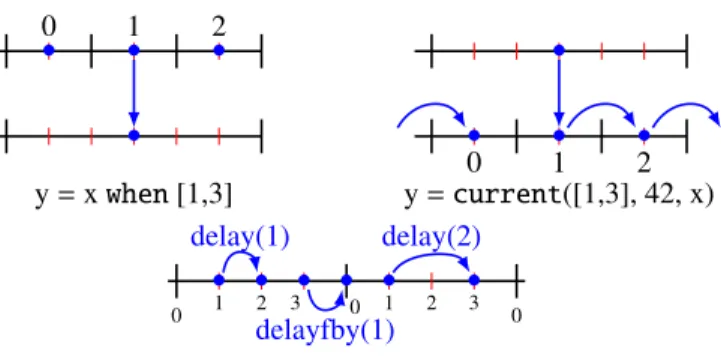
The other different happens at the level of the expression of a model node (exp_m). First, we specialize the when and the current expressions to one-synchronous clocks (cf Figure 2). Instead of having to provide a boolean variable, we give two integers k and ratio. For both expressions, ratio is the integral ratio between the two involved periods (which must be harmonic). For the when expression, because the fast period executes ratio times during one slow period, k specifies which one of these instance is sub-sampled (0 ≤ k < ratio). For the current expression, the fast period repeats the last slow value which is produced and k specifies for which of these fast value the update occurs (0 ≤ k < ratio).
• 0 • 1 • 2 • y= x when [1,3] • • 0 • 1 • 2 y= current([1,3], 42, x) delay(1) • • delay(2) • • delayfby(1) • • 0 1 2 3 0 1 2 3 0
Figure 2: Graphical representation of the when, current, delay and delayfby expressions for 1-synchronous clocks. In the left and right parts, the two periods are 6 and 2 and the bullets are labeled by the value of k needed to select this instance. In the bottom part, the period is 4 and the ticks are labeled by their phase.
Second, the merge expression is not available for these nodes. Indeed, if we try to use it to link two periods of ratio which is more than 2, then the clock of the last branch of the merge is activated more than once per period, thus is not 1-synchronous.
Finally, we have added the delay and delayfby expressions. These expressions do not change the period of an expression, but increases the phase of a given integral value d. The delay expression cannot increase the phase of an expression above its associated period, because we would enter into the next period with no value for the current one, thus we would not have a strictly periodic clock. Instead, we can use the delayfby with an initial value provided on its left and which must cross a period. Also, notice that a fby does not change the clock of an expression, thus it can be seen as a particular case of a delayfby.
3.2
Clocking analysis for 1-synchronous operators
Same period operators Let us consider first the delay and the delayfby expressions. As described previously, these operator delay the phase of the clock by a constant value d. Their clocking rules are:
H ` x:: [k, n] 0 ≤ d < n − k H `delay(d) x :: [k+ d, n]
H ` x:: [k, n] H ` i:: [k+ d − n, n] 0 ≤ k + d − n < n H `i delayfby(d) x :: [k+ d − n, n]
Fast to slow period Let us consider a when expression of period m, whose subexpression is of period n. Because of the harmonicity hypothesis, we have an integer r such that m= n.r. The clocking rule for this operator is:
H ` x:: [p, n] m= n.r q = k.n + p H ` xwhen [k, r] :: [q, m]
Figure 3a explains the relation between the phases of the two clocks. The phase q of the when expression is the sum of (i) the number of phases from the periods of the previous non-sampled instances (k.n), and (ii) of the phase of the subexpression (p). Notice that the relation between p and q is linear.
• • • • k × n + p q (a) y= x when [k,r] • • • • p k × n + q (b) y= current([k,r], 0, x)
Figure 3: Typing rule of when and current operator specialized to 1-synchronous clocks.
model main() returns () var a :: [0,1]; b :: [1,2]; c :: [2,6]; d :: [0,2]; e :: [0,1]; let b = f1(a when [1,2]); c = delay(1) f2(b when [1,3]); d = delay(2) f3(current([2,3], 0, c)); e = f4(current([0,2], 0, d)); tel •a • b • c • d •e
Figure 4: Example of fully specified 1-synchronous program (all phases are known). The black lines correspond to the period boundaries (and a phase value of 0). The red lines correspond to the phases inside a period. The blue arrows show an instance of chain of sub/over-sampling between the 5 variables of the program.
Slow to fast period Let us consider a current expression of period n, whose subexpression is of period m. Again, because of the harmonicity hypothesis, we have a ratio r such that m = n.r. The clocking rule for this operator is:
H ` x:: [p, m] H ` i:: [q, n] m= n.r q = p − k.n H `current([k, r], i, x) :: [q, n]
Figure 3b explains the relation between the phases of the two clocks. The phase p of the subexpression is the sum of (i) the number of phases from the periods of the previous repeated instances (k.n), and (ii) of the phase of the current expression (q). Again, the relation between p and q is linear.
Example Figure 4 presents an example of model node, spawning over 3 periods (1, 2 and 6).
3.3
Code generation
We have several options for the code generation of a 1-synchronous program. We can either translate the model nodes back into classical Lustre node, and plug ourselves into the classical Lustre compilation flow. Alternatively, we can have a specialized code generator strategy, using the exposed properties of the clocks to generate code.
Model to classical node translation Given a model node, we want to convert it into a classical Lustre node: we need to replace the one-synchronous clocks by classical clocks, and to translate the specific 1-synchronous expressions. First, we build the period graph, an acyclic directed graph in which a node is a period of the program, its root is the period 1, and an edge corresponds to a harmonic relation between two periods and is labeled by their ratio. For each when and current expression in the program, there must be a path in the period graph from its fast period to its slow period.
Then, we replace the delay expressions by the combination of a when expression of a current expression. To find the correct clock between these two expressions, we consider the clock [p, n] of a delay expression and its argument d. The common clock is the clock with the slowest period which is the sub-clock of both [p, n] and [p+ d, n]. So, it is [q, m] where m = gcd(d, n) and q = p mod m. Therefore, the substitution is:
(delay(d) e)::[p,n] { (current([(p-q)/m, n/m], i, e)) when [(p+d-q)/m, n/m] This translation is exactly the same for the delayfby expression. Notice that we need to provide an initial value i for the current expression. This value will never be used in the translation of a delay, because we have the guaranty that the clock of the delay always activates after the clock of its inner expression. In the case of a delayfby, this initial value will be used the first time.
Then, we consider the clocks whose period are not a direct child of the root of the period graph, thus which are separated from the root by several intermediate periods. We decompose these clocks into several clocks of smaller periods, using the on construct, such that each clocks corresponds to a single edge in the period graph. For example, [1, 6] is decomposed by [1,2] on [0,3] if the period 2 is between the periods 1 and 6. We perform the same decomposition for the argument of the when (resp. current) expressions, when one of the period of these expressions are not a direct child of the other. For example, if we have (e when [1,10]) :: [2,3] and the period 6 is between 3 and 30 in the period graph, we decompose this expression into (e when [1,2]) when [0,5].
Finally, we build the local periodic clocks (similar to the half variable in the example of Section 2). For each expressions e when [k,r], where e::[p,n], we register the values of the tuple (k, r, p, n) into a set L. Like-wise for the expressions current([k,r], i, e) :: [p,n]. For the periodic clocks which were previously decomposed into a succession of clocks ([p1, n1] on . . . on [pl, nl]), we register the values of the tuples for all intermediate clocks, which are the (pi, ni, Pj<ipj(Qk≤ jnk),Qj<inj), for 1 ≤ i ≤ l.
For each (k, r, p, n) ∈ L, we build a new periodic boolean variable of clock [p, n] and whose values are (FkT Fr−k−1). For example, in Section 2, half is the local periodic clock for the tuple value (0, 2, 0, 1) (its value is (T F) and its clock [0, 1]). We build its corresponding equation from a succession of r fby expressions. We use these new variables to replace the argument of the when and current expressions, and to replace the 1-synchronous clocks in the variables declarations. The main reason we perform this decomposition of local clocks is so that the classical clocking analysis manages to unify clocks.
Specialized code generation Another option is to exploit the property of 1-synchronous clocks to generate specific code. We can use a classical Lustre code generation scheme [4], producing a step and a reset function for the compiled node. The resulting step function will correspond to the base clock: one execution corresponds to one phase of the computation. Also, because of the presence of many clocks, there will be many if statements in the code.
Another option is to produce one specialized step function per different computation which can be performed during a phase. In order to run this computation, the main while loop must cycle through these step functions in order. Because we know precisely which clocks are activated on a given phase, we can remove all the if statements in the generated code. This leads to more efficient code, at the expense of a much larger generated code.
A third option is to unroll the computation and to produce a single step function corresponding to the smallest common multiplier of all periods in the program (called the hyperperiod). The unrolling of the computation can be considered as a program transformation called the hyperperiod expansion. This transformation is a way to remove the multiperiodic aspect of a program. However, the transformation has two drawbacks. First, the duplicated functions must be stateless. Indeed, all the instances of a node in the hyperexpanded program must share the same internal state. Thus, if we have a stateful node, we need to make it stateless by exposing its internal memory as a new input and output beforehand. The initial state is generated by a separated function (similar to a reset function which would be generated in classical Lustre code generation). Through hyperperiod expansion, these states will be shared across instances.
Another drawback is that all the input and output of the state are assumed to be available at the beginning of the hyperperiod. However, in the real world, input and output are not available or made available at the same time. Thus, if we want to run that as a real application, there are other timing requirements to be enforced on the usage of inputs and production of outputs, in the form of scheduling constraints for the statements of the step function.
4
Phase inference
In this section, we study the possibility of under-specifying phases, to dramatically improve the practicality of the language. We present a language extension and show how to extract constraints on the under-specified phases. We study how to solve these constraints in reasonable amount of time for realistic cost functions and scaling to large real-time applications. Once a solution is found, we show how to transform the program back to a classical 1-synchronous Lustre program.
4.1
Omitting phases of 1-periodic clocks
In a 1-synchronous program, the phases of the clocks of a program can also be viewed as a coarse-grain sched-ule. Their values directly affect the quality of the generated code. Moreover, finding a good set of values is a complex problem, which generally depends on other non-functional factors, such as processor architecture and microarchitectural details. However, experimenting with and changing the phase of a node is a heavy operation. Indeed, the phase of a variable also impacts the equation which defines it and all of those that use it. This is a direct consequence of the clocking algorithm enforcing the synchronous composition hypothesis on the program. Also, changing the phase of a variable might introduce, remove or retime a delay operation in many other equa-tions. Therefore, asking a programmer to decide and fix the phases of a program manually is error-prone and unreasonable, especially in the case of large applications and in safety-critical ones.
In order to solve this problem, we introduce the possibility to associate a 1-periodic clock with an unknown phase with a phase variable. This implies the following modification to the syntax presented in Section 3.1:
oneck ::= [ph, per] | [.., per]
exp_m ::= . . . | buffer exp_m | c bufferfby exp_m
We have introduced a new syntax for one-synchronous clocks, where the phase of a clock is not specified and only the period is provided. In term of dataflow (Kahn) semantics, this is still valid and functionally deterministic: the same sequence of values is computed. However, the synchronous semantic is no longer applicable: the tick of the global clock on which the computation of a given value occurs might change, according to a decision taken internally by the compiler.
Because we have variables and expressions with no precise phase, we cannot set a constant length to a delay operator inside a given dataflow equation. Thus, we need to use a more relaxed buffer operator. Thus, we introduce
buffer and bufferfby which are variants of the delay and delayfby operators where the delay is not specified. Notice that the buffer operator is the same used in the N-synchronous model.
4.2
Clocking analysis and constraint extraction
Symbolic phases Because the clocking rules manipulates phases, which might be unknown, we need to introduce some fresh variables (called phase variable) representing the phases of the application. These phases can be manipulated symbolically through the clocking rules, as linear expressions (var+ const), and might issue equality constraints during unification of clocks (in order to ensure that both side of an equation or the arguments of an operator have the same clock). In the rest of the paper, we will use the same notation [p, n] for a 1-synchronous clock, whichever the nature of p is (either a constant or a expression of phase variables).
Clocking rule of the new expressions Because the buffer operator only delays the clock of an expression of an unknown quantity, (i) both clocks must have the same period and (ii) the phase of the clock of the subexpression must be smaller or equal to the phase of the clock of the buffer expression. Its clocking rule is:
H ` x:: [p, n] 0 ≤ p ≤ q < n H `buffer x :: [q, n]
Notice that we now have a constraint p ≤ q between the phase p of the subexpression of the buffer and the phase q of the buffer expression. This is the classical dataflow constraint: the producer must happen before the consumer. During the clocking analysis, we gather these constraints in order to check the coherence of the phases or to solve them if there are unknown phases involved.
The clocking rule of a bufferfby expression is:
H ` x:: [p, n] H ` i:: [q, n] H ` ibufferfby x :: [q, n]
Notice that there is no constraint linking p and q: indeed the value of x used is coming from the previous instance of the period, so the bufferfby expression does not need to wait for anything. If we wish to share the memory of the old value of x and the new one, we have to ensure that the old value of x is used before the new one is computed. This adds the (optional) constraint q ≤ p.
Example We consider again the example of 1-synchronous program given in Figure 4, and now assume that all variables do not have a phase specified. The resulting program and extracted constraints are shown in Figure 5. Non-functional constraints We can enrich the syntax of the language defined in Section 4.1 with annotations that encode additional constraints on the phases. In particular, our compilation flow is able to manage (i) minimal or maximal value constraints (p ≤ M or m ≤ p), (ii) precedence constraints (p1 ≤ p2) and (iii) latency constraints over a chain of dependence (e ≤ L, bounding the number of phases delayed because of the operators of the chain of dependences).
4.3
Constraint resolution and cost function
Form of the constraints There are several sources of constraints on the phases, most of them being exposed through clocking analysis. Before enumerating them, note that the phase of any expression in the program is either
model main() returns () var a :: [..,1]; b :: [..,2]; c :: [..,6]; d :: [..,2]; e :: [..,1]; let
b = buffer f1(a when [1,2]); c = buffer f2(b when [0,3]);
d = buffer f3(current([2,3], 0, c)); e = buffer f4(current([0,2], 0, d)); tel
List of extracted constraints:
• Bounds from variable declarations: – 0 ≤ pa, pe< 1
– 0 ≤ pb, pd< 2 – 0 ≤ pc< 6
• Constraints from buffer clocking rule: – pa+ 1 ≤ pb
– pb ≤ pc – pc− 4 ≤ pd – pd ≤ pe
Figure 5: Example of 1-synchronous program where all phases are unknown. pxis the phase of the variable x.
a constant (typically, if the phase is known), or the sum of a phase variable and a constant. This invariant can be proved by induction, using the different clocking rules. The encountered constraints are:
• The boundary conditions on the phases of the underspecified clocks, which can be extracted from the variable declarations. An annotation imposing a minimal/maximal value can refine it. These constraints have the form m ≤ p or p ≤ M, p being a phase variable and m, M constants.
• The dependence constraints coming from the buffer clocking rules, or precedence annotations. Due to the form of the phases of all sub-expression of the program, there are at most 2 phase variables in these constraints, on opposite side of the inequality and with coefficients of 1. So, these constraints have the form p1+ C ≤ p2, or the form of a boundary condition if one of the compared phase is a constant.
• The latency constraints coming from dependence annotations. If the considered dependence chain has only one edge, the constraint has the same form than a dependence constraint. Else, an arbitrary number of phase variable might occur in these constraints.
• The unification constraints, which are equalities coming from the equations and the application. Because we will always have a phase variable with a coefficient of 1 in this equalities, we can use them as substitution to reduce the number of phase variables of the system of constraints. Therefore, we can safely ignore them. Resolution of the constraints If we do not have complicated latency constraints, then all constraints are di fference-bound constraints. Thus, we can use a Floyd-Warshall algorithm [8] to solve them. We pick by default the solution composed of the minimal feasible value for each phase variables, which corresponds to scheduling every compu-tation at the earliest. If the constraints are more complicated, we need to rely on an ILP solver to find a solution. Cost functions The selected phase values is a coarse-grain schedule of the application, so selecting an arbitrary solution might have a negative impact of the performances. Therefore, we wish to consider other criteria, such as memory allocation or load balancing across the phases.
These criteria are encoded in our problem as a cost function, which will try to optimize it through ILP. In many case, getting an optimal solution is much more than needed, and just finding a solution which balances the workload well enough to fit a real-time constraint, or save enough memory to fit in a hardware memory, is enough.
Memory cost function We can consider a cost function which minimizes the memory used by the bufferfby expressions. This is done by using the optional constraint of the bufferfby expression, and by conditioning its activation using a binary variable δ. A binary variable is an integral variable which can be either 0 or 1. If the original constraint is q ≤ p, the new constraint will be q ≤ p+ δ.per, where per is the period of the bufferfby expression (which dominates all possible value of q in this constraint). We can easily see that this constraint is voided when δ = 1. This means that when δ = 1, there are not possible reuse of the memory of a bufferfby. Therefore, the cost function is the summation of all the δ of the program: minimizing this cost function corresponds to maximizing the number of δ equal to 0, thus the number of constraints satisfied.
WCET load balancing cost function An interesting cost function when mapping the application into a sequen-tial architecture is the WCET load balancing. Each node is associated with a weight (corresponding to its WCET) and the goal is to balance it across all phases of the application, so that it fits in the allocated time for every phase. The phase pTof a node T is the phase shared by its output variables. WT is the weight of the node T (WCET in our case). In order to encode the sum of the weights of the nodes scheduled on a given phase, we need to introduce a dual binary encoding of the integral phase variables. We introduce, for all node T and possible phase k, a binary variable δk,T which encodes if a node T is scheduled at phase k. We also introduce a final integral variable Wmax which is also our cost function to minimize. The list of additional constraints introduced by the load-balancing is:
(∀T ) P k
δk,T = 1 (unicity of the 1 value) (∀T ) P
k
k.δk,T = pT (link integral-binary) (∀k) P
T
(δkmod period(T ),T × WT) ≤ Wmax (max weight)
Binary WCET load balancing We have a variant of this cost function, called binary WCET load balancing, where we only use the binary variables in place of the integral phase variables. This avoid two sets of variables representing the same information, and it can be solved faster in some situations. The main issue is to translate the constraints on the integral variables (dependences or latency) into an equivalent set of constraints on binary variables. If the constraint is a difference-bound constraint (which is the case for all dependence constraints), the translation is straight-forward:
p ≤ q+ C { (∀k) δp,k≤ X
l≥k+C δq,l
In the case of complicated latency constraints with more than 2 phase variables, we have at least a phase variable q whose coefficient is 1 that we can isolate from the rest of the constraint:
X
k
ck.pk≤ q
We introduce a new integral temporary variable e = Pkck.pk, and we consider its binary variables (δe,k)k. The constraint becomes e ≤ q, which is translatable using the straight-forward case. We still need to translate the equation e= Pkck.pk. We consider all combination of values (vk)kof the pks, and by classifying the combination according to the value V of e it corresponds, we obtain the following constraint using the binary variable:
(∀V) X (vk)k P kck.vk= V Y k δpk,vk = δe,V
These constraints are polynomial, however it is possible to transform them into affine constraints by the fol-lowing way:
(∀(vk)k) X k
δpk,vk − (card(vk) − 1) ≤ δe,V, where V=
X
k ckvk
This translation works because we have a single δe,kthat is equal to 1 (unicity constraint), and there is exactly one combination vk such that all δpk,vk are also 1. For this combination, the sum
P
kδpk,vk will be equal to the
number of vk, thus δe,V will be forced to be 1. For all the other combinations, we havePkδpk,vk < card(vk), thus
their corresponding δe,Vis not constrained.
For example, let us consider the constraint p1+ p2 ≤ p3, where 0 ≤ p1 < 2, 0 ≤ p2 < 2 and 0 ≤ p3< 4. We introduce the new temporary variable e= p1+ p2. The constraint becomes e ≤ p3which can be translated in the straight-forward manner. We still have to translate the equalities, and the constraints on it are:
δp1,0.δp2,0= δe,0 δp1,1.δp2,0+ δp1,0.δp2,1= δe,1 δp1,1.δp2,1= δe,2
After transformation, we have the following set of linear constraints on binary variables: δp1,0+ δp2,0− 1 ≤ δe,0 δp1,1+ δp2,0− 1 ≤ δe,1 δp1,0+ δp2,1− 1 ≤ δe,1 δp1,1+ δp2,1− 1 ≤ δe,2
These constraints are affine, thus can be solved by an ILP solver.
4.4
Experiments
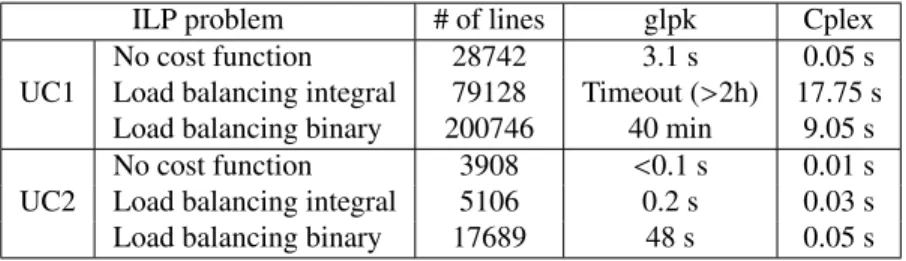
Description of the use cases We consider two real-world avionic integration program as our use cases. The first use case (called UC1) is composed of 5124 Lustre nodes and 32006 variables. This application has 4 harmonic periods (1, 2, 4 and 12, corresponding to 10, 20, 40 and 120 ms) and each node are activated exactly once per period. We also have a WCET associated to each node of the application. The nodes of this application are already scheduled across phases, but we intentionally forget this information for our experiment. There are no latency constraints on this application.
The second use case (called UC2) is composed of 142 Lustre nodes. This application has 5 harmonic periods (1, 2, 4, 8 and 16, corresponding to 15, 30, 60, 120 and 240 ms). Each nodes are activated exactly once per period. This UC was implemented as a hierarchy of Scade nodes, and did require a lot of normalization steps to extract a suitable dependence graph. Because the situation of this application is common (its nodes are generated from a collection of hierarchical Scade sheets), we take the time to summarize these normalization steps:
• First, we expose the parallelism of the application in the top most node. This is done by successive recursive inlining of the nodes, in order to have all equations under the same node. The depth of this recursive inlining transformation controls the granularity of the parallelization. In our case, we choose to inline all integration nodes, i.e., “administrative” nodes which contains only function calls and data structure manipulation, but no computation by themselves.
• Then, in order to remove false dependences, we destruct all the arrays of the application into their elements. However, the nodes called by the main node have arrays as inputs and outputs. Thus, for each of these nodes,
ILP problem # of lines glpk Cplex UC1
No cost function 28742 3.1 s 0.05 s
Load balancing integral 79128 Timeout (>2h) 17.75 s Load balancing binary 200746 40 min 9.05 s UC2
No cost function 3908 <0.1 s 0.01 s Load balancing integral 5106 0.2 s 0.03 s Load balancing binary 17689 48 s 0.05 s
Figure 6: Time spent by solvers to find a valid phase solution for the 2 use cases and three cost functions. The glpk results were obtained from a local installation. The Cplex results were obtained from the NEOS servers.
we create a corresponding scalarified node with scalars as inputs and outputs, which internally builds the array, calls the original node, then deconstructs the output arrays. We substitute the original nodes by the scalarified node in the integration program, so that we can destruct all the remaining arrays of the program. An alternative approach was explored, in which the scalarified nodes were built later in the compilation flow, by aggregating equations. However, it did not give convincing results.
• The clocks are encoded through conditional activation (condact operator), taking as an argument one of the 41 boolean variables produced by a sequencer node (scheduled on the base period). These boolean variables are 1-synchronous clocks, computed by a modulo. We manually flagged the values produced by the sequencer node with its corresponding 1-synchronous clock information.
Interestingly, two of these clocks have a different phase according to a boolean input. In order to manage this case, we overapproximate the execution of the corresponding computation node, by splitting it into two instances of the same node, both scheduled into the 2 different phases. Internally, we can add a condition on the boolean input to know if we should activate this node for a given phase.
• Finally, we perform various normalization steps on the program, such as the removal of the copy equations, deadcode elimination or constant propagation.
Once these preprocessing steps are realized, our main node only contains function calls and fby equations. We extract the dependence graph and, once more, intentionally forget this information for our experiment.
Experiment: scalability of the ILP solving Given the dependence graph of two applications, we used a proto-type to generate the set of constraints on the phases, according to different cost functions. We evaluate the time spent by a ILP solver (glpk [1] and Cplex2) on these problems, to estimate the feasibility of our compilation flow.
Figure 6 shows the time spent by the two solvers to find a phase solution for the 3 variants of the ILP formulation of the two use cases. We can draw two conclusions from these numbers: (i) it is possible to find a solution in a reasonable time (less than a minute) for a very large real-world application; (ii) none of the variant for the load balancing function is faster than the other in general. This might be caused by the fact the UC2 is a magnitude of order smaller than the UC1. Therefore, both versions are pertinent.
4.5
Substitution of the phase solution
Once a set of valid values for the phases of the program is found, we use these values to obtain a classical 1-synchronous program, in which all phases are known. This is done by completing the clock of all variable dec-larations and by transforming all buffer into delay (resp. bufferfby into delayfby). Given a phase solution S, which is a mapping from a phase variable px(of variable x) to a valid value v, the transformation rules of this transformation are:
x:type::[..,n] { x : ty :: [v,n], where S(px)= v
e::[f(p1, . . . , pr),n] { e::[f(S(p1), . . . , S(pr)),n], for every expression e buffer e { delay(d) e, where d= q − p > 0,
(buffer e)::[q,n] and e::[p,n] buffer e { e, where q= p,
(buffer e)::[q,n] and e::[p,n] i bufferfby e { i delayfby(d) e, where d= n + q − p
(buffer e)::[q,n] and e::[p,n]
We can verify the validity of the solution while performing this replacement. For example, if the parameter of a delay is found to be a negative number, its corresponding dependence constraint was violated by the solution.
5
Underspecified one-synchronous operators
The previous section proposed an extension where the phases of some clocks are not given, but inferred later by the compiler, by using a ILP. However, such a formalization is still over-constrained for a wide range of real-time control scenarii where it does not matter which value is being consumed as long as this value is “fresh” enough and the computation takes place early enough. The typical example is that of a sensor sampling a physical value with with low temporal variability. Fixing the dataflow arbitrary restricts the set of valid schedules to be explored, and might invalidate potentially interesting schedules. The goal of this section is to express this variability with operators whose incoming dependence is underspecified. Then, we use this information to relax the constraints on the phases, and when the phases are set, to derive a fully specified 1-synchronous program.
5.1
Underspecified one-synchronous operator
We introduce the underspecified one-synchronous operator through an extension of the syntax first presented in Section 3.1, and extended in Section 4.1:
expm ::= . . . | c fby? expm| c bufferfby? expm | expm when? r | current?(r, c, expm)
We have introduced 4 underspecified operators, which are underspecified versions of one-synchronous opera-tors. Their semantic is:
• The value of (c fby? e) can be either (c fby e) or e.
• The value of (c bufferfby? e) can be either (c bufferfby e) or (buffer e). • The value of (e when? r) is (e when [k,r]), for a 0 ≤ k < r.
model loop() returns (y:int) let
x = 0 fby? y; y = 1 fby? x; tel
(a) First example.
model loop() returns (y:int) let
x = 0 fby y; y = x; tel
(b) Determinized first example.
model loop(x:int) returns (z:int) var y:int::[..,2];
let
y = x when? 2;
z = current?(2, 0, buffer y); tel
(c) Second example.
model loop(x:int) returns (z:int) var y:int::[0,2];
let
y = x when [0,2];
z = current([1,2], 0, delay(1) y); tel
(d) Determinized second example.
Figure 7: Examples of underspecified 1-synchronous programs. Notice that the determinized versions are not unique.
The when? operator corresponds to a 1-synchronous when operator for which we do not know which value is sampled. Likewise, we do not know when the update of the fast value of a current? operator happens. Technically, we could build the operators when? (resp. current?) as syntactic sugar from the operator when (resp. current) and a succession of fby? operators on the faster period. However, it is more convenient and meaningful to define them as part of the language. The value of all underspecified operator are taken by the compiler, and fixed during the clocking analysis as part of the solution found for the phases.
Notice that, the very computation performed by the program changes according to this decision. By using these operators, the programmer assumes the compiler that all possible version of the program is correct and lets the compiler pick whichever it prefers.
Figure 7 shows two examples of model nodes using non-deterministic operators, and one of their corresponding deterministic version, which corresponds to any combination of choice that generates a valid program.
5.2
Clocking analysis and constraint extraction
Symbolic decision variables In order to represent which value is selected for a underspecified operator, we introduce new integral symbolic variables d , called decision variables. Due to these new variables, during the clocking analysis, the phases can be general affine expressions, instead of just linear expressions.
Clocking rule of the fby? and bufferfby? expressions Like a fby expression, the fby? expression has the same clock than its subexpression. We still associate a decision variable d ∈ [0, 1] to this operator, such that d= 1 corresponds to a fby and d= 0 corresponds to a simple copy.
The clocking rule of a bufferfby? expression is:
H ` x:: [p, n] H ` i:: [q, n] p ≤ q+ n.d 0 ≤ d ≤ 1 H ` ibufferfby? x :: [q, n]
When the decision variable of bufferfby? d is 1, we have a bufferfby and when it is 0, we have a buffer. Thus, we have to activate the constraint of the buffer only when d = 0. This is done by using the period n of the expressions, which will always be bigger than p.
Clocking rule of the when? and current? expressions The clocking rule of a when? expression is: H ` x:: [p, n] m= n.r q = d.n + p 0 ≤ d < r
H ` xwhen? r :: [q, m]
This is simply the clocking rule of a 1-deterministic when expression, where the index of the sampled value (which was k in Section 3.2) is the new decision variable d.
Likewise, the clocking rule of a current? expression is:
H ` x:: [p, m] H ` i:: [q, n]
m= n.r
q= p − d.n 0 ≤ d < r H `current?(r, i, x) :: [q, n]
Again, this is simply the clocking rule of a 1-deterministic current expression, where the index of the sampled value (which was k in Section 3.2) is the new decision variable d.
Causality constraints The causality analysis ensures that no variable depends on itself, instead of depending on the values from the previous periods. Because the fby? and bufferfby? operators might either use a value of the current instance of period or from the previous instance of the period, they interact with this analysis. If we consider the first example of Figure 7, if none of the two fby? are transformed into a fby, then the resulting program has a causality loop and is not valid. Thus, we wish to add a constraint on the decision variables of the fby? and bufferfby? expressions to reject these programs.
We consider all the loops in the dependence graph of a model nodes:
• If they have a fby or a bufferfby expression, then we are sure to use a value from a past period. No constraint is needed for this loop.
• If there is no fby/bufferfby/fby?/bufferfby?, we are still on the same period and, because there is only one clock activation per period, the value used is the value produced: we have to reject the program. • If there is no fby/bufferfby but there is at least a fby?/bufferfby?, we have to ensure that at least one
of their decision variable is equal to 1. Thus, we generate the constraintP
kdk ≥ 1, where the dkare the decision variables of the encountered fby?/bufferfby?
In the first example of Figure 7, the extracted constraint is d1+ d2≥ 1, where d1is the decision variable of the expression (0 fby? y) and d2the decision variable of the expression (1 fby? x).
5.3
Solving the constraints
Compared to Section 4.3, the constraints are also affine in general. The coefficient in front of the decision variables might be different of 1. If we wish to use the binary version of the load balancing cost function, we can also introduce binary variables for the decision variables. Else, the solving process is strictly identical to the previous section and the solution found also contains values for the decision variables.
5.4
Determinizing the program
As shown in Section 4.5, once a valid solution is found for the phases, one may use it to return to a classical 1-synchronous Lustre program. Before substituting the values of the phases, we use the decision variables to substitute the underspecified expressions by their chosen value. We assume that the chosen solution (D) for the decision variables is a mapping associated a underspecified expression to the value of the decision variable. The corresponding rules of this transformation are:
c fby? e { e if D(c fby? e)= 0
c fby? e { c fby e if D(c fby? e)= 1
c bufferfby? e { c buffer e if D(c bufferfby? e)= 0 c bufferfby? e { c bufferfby e if D(c bufferfby? e)= 1
x when? r { x when [k,r] if D(x when? r)= k
current?(r, c, x) { current([k,r], c, x) if D(current?(r, c, x))= k
At this point, the program is a classical deterministic 1-synchronous Lustre program, and one may carry on with the rest of the compilation.
6
Related work
1-synchronous clocks Smarandache et al. [19] studied affine clocks which are similar to our 1-synchronous clocks, in the context of the Signal language. The formalization does not set bounds on the phase, which means that clocks may have no activations during the first periods at the start of the computation. The authors investigated the clock unification problem, across different periods and phases.
Plateau and Mandel [14, 17] studied the possibility of not specifying the phase of some clocks, in the context of the synchronous model [7]. In [14], the authors extract the constraints on the activation of a general N-synchronous clock in the Lucy-n language [15]. While their formalization generalizes our work, they did not study the scalability of the extracted constraints on large applications, nor did they model real-time load balancing or efficient code generation.
Forget, Pagetti et al [9, 16] introduced Prelude, an equational language aimed at multi-periodic integration program. It proposes three operators to manipulate clocks: /.k (corresponding to a when which samples the first occurrence), *.k (corresponding to a current which updates on the first occurrence) and → (corresponding to a delay and used to orchestrate phases). Some real-time information are encoded in the language, and the nodes are associated with a WCET. In term of scheduling, they adopt the relaxed synchronous hypothesis: the execution of a node must end before the next tick of its clock, and not the next tick of the base clock. Thus, the classical step function code generation strategy, where a step function corresponds to a tick of the base clock, is not applicable. Therefore, the earliest paper on Prelude assumed a preemptive operating systems. However, following papers [5] considered the generation of parallel code, allowing bare metal implementations.
Henzinger et al [13] introduced Giotto, a time-triggered language for multi-periodic integration programs. In their model, drivers are instantaneous computations which are used to communicate between periodic tasks. The periods of those tasks are not required to be harmonic. A driver can be guarded and transmit the last computed value when it is not activated. Finally, they support modes, which can periodically replace the set of tasks of the application with another.
Underspecified operators In Simulink, the rate transition block [2] allows communication between different periods. It can communicate from a fast period to a slow one, or the opposite, which correspond to the when and
current operators. It also has the choice between being deterministic while introducing extra communication delay, or non-deterministic but with a better latency.
Wyss [20] introduced the "don’t care" operator (dc), which corresponds to our fby? operator. He defines the semantic of this operator and studies its impact on the latency requirements, and on the causality analysis and generates a set of pseudo-boolean constraints which are similar to our causality constraints in Section 5.2.
Maraninchi and Graillat [11] have considered bounded non-deterministic delays to deal with the variable communication latency over computation clusters of the Kalray MPPA. They describe a fundamentally non-deterministic system behavior, while our approach uses the same operator to describe a collection of functionally deterministic programs, among which the compiler can pick to optimize the load of a real-time implementation.
7
Conclusion
This paper proposes three variations of the Lustre language. First, the modeling of 1-synchronous clocks, i.e. strictly periodic clocks with a single activation. These clocks allow to explore multiple inference and code gen-eration possibilities. These include the option to relax the synchronous composition hypothesis by not specifying the phases of some 1-synchronous clocks. Dataflow and real-time constraints on these phases are collected in a modular and structural way, and may then be solved at the top level of the integration program.
We also introduce underspecified operators, for which the control flow is underspecified, to further relax the constraints on the phases. This increases the space of valid schedules while exploiting the slack in control au-tomation contexts. We determinize the program once the phases are found. Finally, we present cost functions and algorithms to solve these constraints and evaluate their scalability on two large real-world avionic applications. All the operators and algorithms described in this paper were integrated in an open-source compiler, along with additional syntactic extension to encode several additional constraints on the phases.
As future work, we can improve the automatic selection of the phase solution. Indeed, the WCET load bal-ancing cost function we consider is suitable for sequential architectures. In the context of parallel architecture, we might want to optimize for other criteria, such as minimizing the critical path of the computation inside any phases of the program.
Acknowledgments: This work has been realized as part of the project ITEA ASSUME, then as part of the col-laboration "All-In-Lustre" between Inria and Airbus. We would also like to thank Paul Feautrier for our discussions about the encoding of the ILP problem, and about the solvers used by this paper.
References
[1] Gnu linear programming kit. https://www.gnu.org/software/glpk/. Accessed: 2020-02-07.
[2] Rate transition simulink documentation. https://www.mathworks.com/help/simulink/slref/ ratetransition.html. Accessed: 2020-02-07.
[3] Albert Benveniste, Paul Le Guernic, and Christian Jacquemot. Synchronous programming with events and relations: the SIGNAL language and its semantics. Science of Computer Programming, 16(2):103–149, 1991.
[4] Darek Biernacki, Jean-Louis Colaco, Grégoire Hamon, and Marc Pouzet. Clock-directed modular code generation of synchronous data-flow languages. In ACM International Conference on Languages, Compilers, and Tools for Embedded Systems (LCTES), Tucson, Arizona, June 2008. ACM.
[5] Frédéric Boniol, Hugues Cassé, Eric Noulard, and Claire Pagetti. Deterministic execution model on COTS hardware. In Andreas Herkersdorf, Kay Römer, and Uwe Brinkschulte, editors, Architecture of Computing Systems (ARCS), pages 98–110, Berlin, Heidelberg, 2012. Springer Berlin Heidelberg.
[6] P. Caspi, D. Pilaud, N. Halbwachs, and J. A. Plaice. LUSTRE: A declarative language for real-time pro-gramming. In Proceedings of the 14th ACM SIGACT-SIGPLAN Symposium on Principles of Programming Languages, POPL’87, pages 178–188, Munich, West Germany, 1987. ACM.
[7] Albert Cohen, Marc Duranton, Christine Eisenbeis, Claire Pagetti, Florence Plateau, and Marc Pouzet. N-synchronous kahn networks: A relaxed model of synchrony for real-time systems. SIGPLAN Notices, 41(1):180–193, January 2006.
[8] Robert W. Floyd. Algorithm 97: Shortest path. Communication of ACM, 5(6):345, June 1962.
[9] Julien Forget. A Synchronous Language for Critical Embedded Systems with Multiple Real-Time Constraints. PhD thesis, Institut Supérieur de l’Aéronautique et de l’Espace, November 2009.
[10] Kahn Gilles. The semantics of a simple language for parallel programming. Information Processing, pages 471–475, Aug 1974.
[11] Amaury Graillat. Code Generation for Multi-Core Processor with Hard Real-Time Constraints. PhD thesis, Université Grenoble Alpes, November 2018.
[12] Grégoire Hamon. Calcul d’horloges et structures de contrôle dans Lucid Synchrone, un langage de flots synchrones à la ML. PhD thesis, Informatique Paris 6, 2002.
[13] Thomas A. Henzinger, Benjamin Horowitz, and Christoph M. Kirsch. Giotto: A time-triggered language for embedded programming. In Thomas A. Henzinger and Christoph M. Kirsch, editors, Embedded Software, pages 166–184, Berlin, Heidelberg, 2001. Springer Berlin Heidelberg.
[14] Louis Mandel and Florence Plateau. Scheduling and buffer sizing of n-synchronous systems. In Mathematics of Program Construction, pages 74–101, Berlin, Heidelberg, 2012. Springer Berlin Heidelberg.
[15] Louis Mandel, Florence Plateau, and Marc Pouzet. Lucy-n: a n-Synchronous Extension of Lustre, pages 288–309. Springer Berlin Heidelberg, Berlin, Heidelberg, June 2010.
[16] Claire Pagetti, Julien Forget, Frédéric Boniol, Mikel Cordovilla, and David Lesens. Multi-task implementa-tion of multi-periodic synchronous programs. Discrete Event Dynamic Systems, 21(3):307–338, September 2011.
[17] Florence Plateau. Modèle n-synchrone pour la programmation de réseaux de Kahn à mémoire bornée. PhD thesis, Université Paris XI, 2010.
[18] Marc Pouzet. Lucid Synchrone: un langage synchrone d’ordre supérieur. PhD thesis, Université Pierre et Marie Curie, Paris, France, Nov 2002.
[19] Irina Madalina Smarandache. Transformations affines d’horloges : application au codesign de systemes temps-reel en utilisant les langages Signal et Alpha. PhD thesis, Université Rennes 1, 1998.
[20] Rémy Wyss, Frédéric Boniol, Julien Forget, and Claire Pagetti. A synchronous language with partial delay specification for real-time systems programming. In 10th Asian Symposium on Programming Languages and Systems, pages 223–238, Kyoto, Japan, December 2012.