HAL Id: cea-01952648
https://hal-cea.archives-ouvertes.fr/cea-01952648
Submitted on 12 Dec 2018
HAL is a multi-disciplinary open access
archive for the deposit and dissemination of
sci-entific research documents, whether they are
pub-lished or not. The documents may come from
teaching and research institutions in France or
abroad, or from public or private research centers.
L’archive ouverte pluridisciplinaire HAL, est
destinée au dépôt et à la diffusion de documents
scientifiques de niveau recherche, publiés ou non,
émanant des établissements d’enseignement et de
recherche français ou étrangers, des laboratoires
publics ou privés.
Marina Filipovic, Eric Barat, Thomas Dautremer, Claude Comtat, Simon
Stute
To cite this version:
Marina Filipovic, Eric Barat, Thomas Dautremer, Claude Comtat, Simon Stute. PET reconstruction
of the posterior image probability, including multimodal images. IEEE Transactions on Medical
Imaging, Institute of Electrical and Electronics Engineers, 2018, �10.1109/tmi.2018.2886050�.
�cea-01952648�
PET reconstruction of the posterior image
probability, including multimodal images
Marina Filipovi´c, ´
Eric Barat, Thomas Dautremer, Claude Comtat, and Simon Stute
Abstract—In PET image reconstruction, it would be useful to obtain the entire posterior probability distribution of the image, because it allows for both estimating image intensity and assessing the uncertainty of the estimation, thus leading to more reliable interpretation. We propose a new entirely probabilistic model: the prior is a distribution over possible smooth regions (distance-driven Chinese restaurant process), and the posterior distribution is estimated using a Gibbs MCMC sampler. Data from other modalities (here one or several MR images) are introduced into the model as additional observed data, providing side information about likely smooth regions in the image. The reconstructed image is the posterior mean, and the uncertainty is presented as an image of the size of 95% posterior intervals. The reconstruction was compared to MLEM and OSEM algorithms, with and without post-smoothing, and to a penalized ML or MAP method that also uses additional images from other modalities. Qualitative and quantitative tests were performed on realistic simulated data with statistical replicates and on several clini-cal examinations presenting pathologies. The proposed method presents appealing properties in terms of obtained bias, variance, spatial regularization, and use of multimodal data, and produces in addition potentially valuable uncertainty information.
Index Terms—PET, image reconstruction, posterior probability distribution, uncertainty, multimodal, MCMC sampler, Bayesian inference, spatial regularization.
I. INTRODUCTION
M
OST iterative reconstruction methods formulate an objective function relating the observed (i.e. acquired or measured) data to the unknown image. The reconstructed image is equivalent to a minimum or maximum solution of this objective function, found using numerical optimization methods. The reconstruction problem is ill-posed and the so-lution may not be unique. In the context of PET reconstruction, the maximum likelihood - expectation maximization (MLEM) based algorithms are widespread. Improvements may aim at accelerating convergence (e.g. OSEM), or at reducing the noise and the partial volume effect in the image by introducing some spatial or temporal regularization. A thorough review of existing iterative methods can be found in [1].In the MLEM PET reconstruction method, the observed data are modeled as a random variable, where the randomness is due to the emission detection process. However, the image being reconstructed (emission concentration) is regarded as
M. Filipovi´c, C. Comtat and S. Stute are with the Imagerie Mol´eculaire In Vivo, IMIV, CEA, Inserm, CNRS, Univ. Paris Sud, Universit´e Paris Saclay, CEA-SHFJ, Orsay, France e-mail: marina.filipovic.work@gmail.com
´
E. Barat and T. Dautremer are with CEA, LIST, Laboratory of Systems Modelling and Simulation, Gif-sur-Yvette, France.
Copyright (c) 2018 IEEE. Personal use of this material is permitted. However, permission to use this material for any other purposes must be obtained from the IEEE by sending a request to pubs-permissions@ieee.org.
deterministic and fixed. As the solution may not be unique, and as the MLEM estimator variance increases with con-vergence, some methods introduce additional constraints and prior assumptions which can drive the final solution into some desirable direction. These methods have two interpretations leading to equivalent algorithms: 1) the image is deterministic, but a penalty term is added to the maximum likelihood objective function (penalized ML) 2) the image is a random variable, and the solution corresponds to the maximum of the posterior distribution (maximum a posteriori or MAP). The spatial regularization is driven by the acquired PET data, and possibly by additional images from other modalities, that might show a better delineation of tissues.
A common assumption is that PET emission concentration is likely to be smooth or homogeneous in some anatomically delimited areas (e.g. gray matter, white matter, organs). When used for PET reconstruction, CT and MRI information is often described as anatomical, because it tends to highlight more anatomical features and may provide better spatial resolution and more contrast between some tissues. Different modali-ties and imaging parameters highlight different morphological and/or functional features of the imaged tissues and possibly different types of edges, especially when they are targeted at specific pathologies. A variety of methods using CT or MR images have been proposed, as reviewed in [2]. Some interesting methods and comparisons between them can be found in [3], [4] and [5], the latter using a generalized equation framework that unifies a large family of algorithms.
All of these methods focus on a single optimal solution and do not deal with posterior probability distribution aspects. However, some theoretical work has been done regarding statistical uncertainty properties (bias, variance, noise prop-agation) of ML (e.g. [6]) and penalized ML algorithms (e.g. [7]).
Few groups have explored more in depth the random nature of Bayesian models, i.e. using sampling methods to recover the entire posterior probability distribution of the image instead of a single solution. The main advantage of estimating the whole posterior distribution is to obtain uncertainty information from all the processes involved, i.e. from the observed data, from the measurement noise and the background signal (e.g. random and scattered coincidences), from the reconstruction process itself, and also possibly from hyperparameters (parameters of the prior). In visual interpretation of the reconstructed image, the uncertainty can be displayed simultaneously to provide information about the reliability of voxel intensities: an es-timated voxel intensity comes with its range. The posterior distribution has also been used to estimate the scanning time
necessary for obtaining an image with a defined reliability in [8], or to perform statistical tests for a specific diagnostic task in [9]. The main difficulties for sampling the posterior consist in building the sampler (deriving equations and choosing sampling strategies and parameters), and in dealing with the computational load. Markov chain Monte Carlo (MCMC) samplers are widely used.
At the very beginning of the development of MAP meth-ods, the solution was approached stochastically using MCMC samplers and simulated annealing in [10], this algorithm being midway between objective function optimization and posterior sampling. In [11] and [12], SPECT reconstruction was performed by sampling the joint posterior probability distribution of the image and of the hyperparameters, using a Gibbs/Markov Random Field (MRF) prior and Metropolis-Hastings (MCMC) samplers on simulated and phantom data. In [13], a Gibbs sampler was built for PET reconstruction, with a nonparameteric Dirichlet Process Mixture prior, which was spatially continuous and thus implied some spatial regulariza-tion. The results were tested on simulated data and compared to MLEM and to a MAP method. Using a similar model, statistical tests were performed on the posterior distribution in [14] and the method was applied to clinical data. In [15], an other random model, named ”origin ensembles recon-struction”, was built for PET reconstruction. A Metropolis-Hastings sampler was used to sample a probability distribution which is formally neither the posterior nor the likelihood. The resulting mean image was shown to be related to a maximum likelihood solution, and the method was tested on simulated data. The same author [9] built a relationship between this distribution and the posterior distribution, for different priors, and performed statistical tests for detection tasks on simulated data. In [8], a more recent Riemann manifold MCMC sampler was used for PET reconstruction because of its suitability for high-dimensional models with highly correlated variables. The prior was non informative, and the tightening of posterior distribution was used as a reconstruction reliability indicator for estimating the required patient scan time.
In this paper, we present a new probabilistic PET reconstruc-tion model, called ”Random Clustering Prior - Gibbs Sampler” (RCP-GS), that seeks to infer the entire posterior probability distribution of the imaged emission concentration. It uses also additional data coming from other modalities, which was not the case with previous methods. The term clustering here refers to spatial clustering of adjacent voxels into homoge-neous areas, which are sometimes also called ’supervoxels’ in image processing literature. The prior is a distance-dependent Chinese Restaurant Process (ddCRP) [16], which represents here a probability distribution of possible spatial clusterings of image voxels into uniform or smooth areas. This is a true prior, especially compared to MAP methods, in the sense that no PET nor MRI observed data are used in the construction of the prior itself. The observed data in the model are the acquired PET raw data, and any amount of additional coregistered, already reconstructed images of any type (here we use one or several different MR images). The posterior probability distribution is sampled using a Gibbs (MCMC) sampler. This reconstruction approach belongs to the domain of Bayesian
inference, and in the tomographic reconstruction community it has been referred to as ”fully Bayesian”, to mark the difference with respect to MAP methods that are often called Bayesian. We avoid using the label Bayesian here because it has different meanings in different contexts and can be confusing. The proposed reconstruction is analyzed and compared to reference methods (MLEM, OSEM, and a MAP (Penalized ML) method which uses an MR image, called MR-MAP from now on) using both simulated and clinical static data. Simulations are built with reality in mind (real scanner description, attenuation, scatter and random rate) [17], producing repeated acquisitions (statistical replicates), and the clinical data come from various patient examinations from the Signa PET/MR scanner (GE Healthcare, Milwaukee, WI, USA).
II. THEORY
The probabilistic model is based on all the assumptions used in MLEM PET reconstruction: independent Poisson distribu-tions (likelihood) for the measurements (counts detection), system matrix, additive contribution of random and scattered coincidences, and use of complete data, i.e. the random variable representing the number of true unscattered counts detected in a line of response and originating from a voxel.
A. The prior
The ddCRP prior distribution models two aspects: grouping of voxels into homogeneous regions or clusters, and assign-ment of an intensity to each cluster (all the voxels belonging to a cluster have the same intensity). Each ddCRP sample represents thus a random spatial clustering of the image, where each cluster is assigned a single random intensity. The main assumptions introduced by this prior are: i) the clusters are built out of neighbour (adjacent) voxels, ii) an indirect prior information is introduced about approximate average size of clusters. Drawing samples from this distribution can be done using a dedicated Gibbs sampler, described in [16]. The sampling process itself gives a good understanding of how the prior works and how it models the image.
1) The spatial clustering: First, voxels are grouped into clusters (uniform regions) by using links c between voxels (a cluster is composed of linked voxels). For each voxel, a categorical distribution (multinomial distribution with a single trial/experience) is built for drawing a single link toward a neighbour voxel or onto the voxel itself. So the possible outcomes for this distribution are link destinations, with the following probabilities: i) the probability of drawing a link from the current voxel onto itself (meaning that the voxel either stays independent or does not include other voxels into its current cluster) is equal to a free parameter or hyperpa-rameter α, divided by the sum of all the link probabilities for this voxel, ii) the probability of drawing a link to any neighbourhood voxel is equal to 1, divided by the sum of all the link probabilities for this voxel.
The hyperparameter α has an indirect influence on the overall average size of the clusters: the tendency would be the larger the α, the smaller the clusters in average.
2) The intensity: When the links c are drawn for each voxel, we get a sample of voxel clustering into uniform regions (i.e. a clustering sample). Then, if λsis the cluster intensity, for each
cluster s we can draw an intensity sample from a previously defined prior probability distribution of cluster intensity p(λs).
This distribution is independent of the clustering process, and has to be chosen according to the properties of PET images. We chose a Gamma distribution, Gamma(a, b), for several practical and realistic reasons: i) the Gamma distribution has the convenient property of being the conjugate prior for the Poisson likelihood, which means that the equations become simpler (the posterior cluster intensity distribution can be expressed analytically as another Gamma distribution), ii) it ensures the non-negativity of the reconstructed image intensity, and iii) by choosing appropriate values for its shape parameter a and rate parameter b, the Gamma distribution is able to approximate various other distributions, such as uniform or other non informative or low informative distributions.
B. The posterior distribution and its sampler
Let yi be the observed number of counts acquired in the
line of response (LOR) i, nij the complete data (number of
true unscattered counts detected in LOR i and emitted in voxel j), qithe additive contribution of random and scattered counts
for LOR i, Aij elements of the system matrix (including all
the scaling and correction factors, e.g. acquisition duration time, calibration factor, projector coefficients with or without TOF weights, attenuation, detector efficiency), λsthe intensity
(emission concentration in Bq per volume) of the cluster s, and c the spatial clustering of the image, implemented using links between neighbour voxels. Additional observed data from other modalities m represent the intensity of already reconstructed MR images. As all the voxels in a cluster have the same intensity, individual voxel intensity is noted λj and
stems from the variables (λs, c), as λj = λs3j.
The posterior distribution for the model is thus p(λ, c, {n, q}|y, m), where λ and c fully describe the reconstructed image. A Gibbs sampler requires conditional probability distributions for each posterior variable given all the other variables. These conditional distributions are then sampled one after another iteratively, and a single iteration produces a sample of the posterior distribution. Below are given the three conditional distributions required for our model, for the posterior variables λ, c and {n, q}. The complete summary and derivations for the Gibbs sampler are given in the Appendix. Some variables become irrelevant for some probability distributions, so they will be omitted when appropriate for simplifying the notation of equations.
1) Step1: The conditional posterior probability of the com-plete data and random/scatter contribution p(n, q|λ, c, y) is derived directly from basic assumptions used for MLEM PET reconstruction. For each LOR observation yi, we build a
multinomial distribution with yi trials, where the outcomes
are all the relevant voxels j belonging to the LOR i and the source of random and scattered counts qi (see the derivation
in the Appendix A). In other words, each count, detected at LOR i, is randomly backprojected into one of the possible
emission origins, i.e. either into one of the relevant voxels j, or into the source of random and scattered counts qi. Outcome
probabilities are determined using the system matrix and the random/scatter expectation ¯qi, as
Aijλj
P
kAikλk+ ¯qi
(1) for the voxels, and
¯ qi
P
kAikλk+ ¯qi
(2) for random/scatter contribution.
2) Step2: The conditional posterior probability distribution of the spatial clustering (links) p(c|n, m) is implemented using a dedicated Gibbs sampler presented in [16]. It is similar to the sampler of the ddCRP prior distribution (described in section II-A), except that now the observed data are introduced. The main difference in the sampling procedure is the probability of drawing a link between two voxels that do not belong to the same cluster, i.e. a link that will cause two distinct clusters s1 and s2 to merge. This probability conveys how likely the
merging of the two clusters is, depending on the samples of all the other variables, and depending on actual observations (i.e. acquired data). The complete derivation is given in Appendix B and follows the procedure described in [16]. The probability of a link that causes two clusters to merge, when the PET observed data are taken into account, is given in Eq.3:
Γ(ns1+ ns2+ a) Γ(ns1+ a)Γ(ns2+ a) (As1+ b) (ns1+a)(A s2+ b) (ns2+a) (As1+ As2+ b) (ns1+ns2+a) (3) For brevity, bold symbols are used for representing sums of variables over some dimensions, for instance the sensitivity for voxel j is noted Aj =PiAij, and the sum of nij for a
cluster s becomes ns=Pi
P
j∈snij.
In order to include MR images as observed data providing information about the spatial clustering part of our model, each MR image must also be represented by a probabilistic model. Here we use a Gaussian random model for each MR image (both prior and likelihood and therefore also the posterior are Gaussian). σ is the known (estimated) standard deviation of MRI observation noise, Ns1 is the number of voxels in
the cluster s1, ms1 being the sum of observed MR image
intensities for the cluster s1, and ρ the ratio of noise standard
deviation to image prior standard deviation (see Appendix B for details). The probability of a link that causes two clusters to merge, when MR observed data (one MR reconstructed image) are taken into account, is given in Eq.4:
1 ρ s Ns1Ns2 Ns1+ Ns2 e− 1 2σ2( ms2 Ns2− ms1 Ns1) 2 Ns1 Ns2 Ns1 +Ns2 (4)
The final probability of a link that merges two clusters, including both PET and MRI data, is simply the product of PET and MRI contributions (Eq.3 and 4), because these prob-abilities are mutually independent. It is thus straightforward to build this model either only with PET data, or with as many additional independent images as advisable.
We introduced a small empirical modification of ddCRP posterior sampling, by making a further distinction regarding neighbourhood voxels: if a neighbour voxel belongs to the same cluster as the current voxel, the link probability is no longer equal to 1 but to α (divided by the sum of all link probabilities). This means that, for a voxel, the probabili-ties are the same for drawing a link into itself and into a neighbour voxel that already belongs to the same cluster. This is considered appealing because both these outcomes have a similarly low impact on the clustering sample, and mainly produce unnecessary permutations of voxel links inside the same cluster.
3) Step3: The conditional posterior probability distribution of cluster intensity p(λ|c, n) can be built independently for each cluster s, which results in a Gamma distribution with the following shape and rate parameters (see the Appendix C for derivation).
p(λs|nj∈s) = Gamma(ns+ a, As+ b) (5)
As the expectation of a Gamma distribution is the ratio of its shape and rate parameters, the expectation of the posterior conditional cluster intensity is equal ns+a
As+b. The influence of
the prior parameters on the final reconstructed image intensity is thus explicit: the influence is smaller if the parameters are small, it decreases when cluster size or the number of counts in a cluster increase, and it increases in small clusters with few observed counts.
An image sample is obtained after successively sampling the three conditional probabilities. Each iteration of the sampler produces a new sample, but the first iterations are discarded, because a MCMC sampler requires a so-called burn-in period (a certain number of iterations) to converge to the actual posterior distribution that it is designed to sample. It should be noted that the notion of sampler convergence is different from the usual notion of convergence when solving for a min/max of objective functions. A sampler converges when it starts producing samples that correspond to the targeted posterior probability distribution. After the convergence, the sampler should be iterated as long as possible, in order to produce enough samples for depicting accurately the whole posterior distribution. To this purpose, the sampler has to ’mix’ well: change has to occur between subsequent samples, so that the produced samples span the whole range of possible values and do not get stuck or restrained to a small area.
C. Interpretation of the model
The properties and purposes of this model can be sep-arated into three distinct categories: i) providing valuable uncertainty information thanks to the fully probabilistic nature of the model, ii) performing spatial regularization thanks to the ddCRP prior, which is a distribution featuring spatial regularization suitable for fully probabilistic models, and iii) including additional information about locally smooth areas thanks to the possibility of including supplementary observed data, e.g. MR images.
Regarding the final reconstructed image, there are several possibilities for choosing an image estimator from the pos-terior probability distribution. In this study we focused on posterior expectation, estimated by averaging the samples. The final PET image represents therefore an average of generated samples of clustering and cluster intensities.
It is interesting to explore the relationship between the proposed model (RCP-GS) and the MLEM model. In order to approximate the MLEM model with our model, the prior distribution of cluster intensity should approximate a uniform distribution, for instance by setting the prior Gamma param-eters to a = 1 and b = 0. Then, the maximum likelihood solution would correspond to the mode (the maximum) of the cluster intensity posterior distribution (Eq.5), which in this setting would be ns
As, according to the formula for Gamma
distribution mode. This estimation has an intuitive interpreta-tion, as shown in [15]. The notable differences with respect to MAP methods are that i) the MRI data are not included in the prior and ii) the final image estimation is based on the posterior mean and not on the posterior mode or maximum.
The observed data in this probabilistic model are PET raw data containing detected counts, formatted either in sinogram or in list mode, and already reconstructed MR images. The PET data contain observations about both spatial uniformities and intensities in the PET image, whereas MRI data contain observations about spatial uniformities and intensities in the MR image. So the meeting point of PET and MRI in the model are the homogeneous regions (clusters). Each clustering sam-ple should be composed of clusters shared by both modalities, and of clusters specific to each modality. Thus, the MR images have an influence only on the clustering part of the model.
It should be noted that PET observations are indirect, because a reconstruction inverse problem lies between the acquired data and the reconstructed image. On the contrary, MR images are already reconstructed and so represent direct observations. The noise in MR observations tends to be lower than in PET observations. One could say that, over sampler iterations, two processes unfold in parallel: the sampler con-vergence to the true posterior distribution, and the solving of the PET reconstruction inverse problem. The first conditional probability requires an initial PET image estimation, similar to conventional reconstructions. Hence, if a uniform initial PET image is supplied to the sampler, the PET probabilistic model is rather inconsistent in the first iteration, whereas the MRI probabilistic model is rather consistent from the start. This unbalanced initial status of the models may be disadvantageous for the PET, because in the first iterations the MRI may have a stronger influence on the clustering part of the model. To even out the initial influence of PET and MRI observed data, we introduced the following feature: the MRI data start playing a part in the model only after a certain number of iterations, after the PET model has already become more consistent (i.e. when the solving of the inverse problem has already progressed). It should be noted that the tuning of the α parameter depends on whether additional information about spatial smoothness (MR images) are included or not. If the α parameter is tuned with the MR image in mind, and the MR image is included after a certain number of iterations,
the α value is less adapted for the first iterations. This is not deemed an issue because the main purpose of the first iterations is to make rough progress towards inverse problem solving.
The uncertainty contained in the posterior distribution is conveyed through an image of the size of 95% posterior inter-vals, computed empirically: for each voxel, generated posterior intensity samples are used to build an interval containing 95% of sampled intensity values, by selecting a lower bound at the 0.025 quantile and a higher bound at the 0.975 quantile. Then, for each voxel, the size of the posterior interval is computed as higher bound minus lower bound, and presented as an image. By definition, the 95% (Bayesian) posterior interval is the interval on the posterior distribution that contains the true voxel intensity with a probability of 0.95. It is closely linked though not equivalent to (frequentist) confidence intervals, which by definition contain the true voxel intensity in 95% of repeated experiences. There are various theoretical and empirical methods for estimating both kinds of intervals. [18] and [19] provide interesting discussions on the relationships between these intervals and on the complementarity and the interaction of frequentist and Bayesian approaches to intervals in applied statistics. It should be noted that the actual coverage properties (95 or other percentage) will be fullfilled for ideal models, that fit the data and the reality perfectly and do not result in ill-posed inverse problems. When dealing with realistic data, the models (i.e. MLEM, MAP, RCP-GS) fit the data only to some extent, so the ideal estimation properties regarding bias, variance, intervals coverage, model fitness, etc. can only be approached asymptotically. In addition, the estimation of posterior intervals is closely linked to bias and variance properties of the estimation of image intensity.
III. MATERIALS AND METHODS
First, we present all the implementation and validation details that are global and common to both simulated and patient data. Second, we present the details that are specific to each type of data.
All the reconstruction methods, the proposed and the ref-erence algorithms, were entirely implemented using the CAS-ToR (Customizable and Advanced Software for Tomographic Reconstruction) platform in C++, [20], [21].
A. General implementation
Concerning the Gamma prior for cluster intensity, we chose its parameters such as to approximate a distribution which contains as few prior information about the cluster intensity as possible. There are various non-informative prior distri-butions, which bring no or few information into the model, e.g. a uniform distribution, Jeffreys priors [22]. We opted for the Jeffreys prior that is built for Poisson likelihood: p(λs) ∝ λ
−1
2
s . To approximate this distribution, the Gamma
prior shape parameter is set to a = 0.5 and the Gamma rate parameter to an arbitrary very small value b = 10−18. It should be noted that in this study, from now on, these prior parameters are regarded as fixed, and are not treated as free prior parameters (hyperparameters) in the model. The
implementation used double floating point precision, and some numerical optimizations and checks were made to minimize the loss in precision due to floating point operations. The voxel neighbourhood for the ddCRP was defined as minimal: it consisted of adjacent voxels on each axis, without diagonal neighbours, so 4 neighbours for 2D images and 6 neighbours for 3D images.
We observed that the sampler had some difficulties mixing and converging to the posterior distribution (the samples changed slowly and depended on the initialization of random generators), which is not a rare issue in MCMC samplers. Taking also into account the required computation time, we opted for an empirical solution: the sampler was run several times in parallel starting from different random initializations. The main criteria for choosing the number of sampler iter-ations, runs, the burn-in period and the number of samples used for building the final posterior distribution, was to assess empirically when the change in the posterior mean image (averaged over all the runs) becomes negligible.
The performance and the characteristics of the proposed re-construction method were analyzed and compared to standard reconstruction methods (MLEM for simulated data and OSEM for clinical data) and to a reference MR-MAP method. Among the variety of MAP methods, we chose a Gibbs or Markov random field (MRF) prior which includes an MR image, with the following features: the relative differences potential function [23], Euclidian distance proximity weights, and Bow-sher similarity weights based on a single MR image [24]. These features were chosen because they have been used and tested often in the literature, and because they present some advantages: the Bowsher similarity weights are simple and do not require any preprocessing nor segmentation of the MR image, and the relative differences potential function allows for some edges and is differentiable. The implementation followed [5] in terms of the optimization algorithm (Green’s one-step-late MAP-EM) and in terms of Bowsher weights. There are 4 parameters or hyperparameters for this MAP method: the size of the neighbourhood Nj, defined here with a sphere whose
radius is given in mm and not in voxels, the parameter β weighting the whole penalty, the parameter γ which regulates the tolerance of edges in the relative differences potential function, and the number of ’most similar’ voxels in the neighbourhood for the Bowsher similarity weights, defined here as a percentage of the (fixed) number of voxels in the predefined neighbourhood. The logarithm of the penalty is thus given by Eq.6, where wjk is the Bowsher weight (0 or 1) for
voxel j and its neighbour k, and djk is the Euclidian distance
between voxels j and k:
−βX j X k∈Nj 1 djk wjk (λj− λk)2 (λj+ λk) + γ|λj− λk| (6)
All the reconstructions were fully quantitative: they took into account all the correction factors (attenuation, random and scattered coincidences, detector efficiency, dead time correction, etc.). There was no system resolution modeling in the reconstructions.
The reconstructions were run on a Dell station PowerEdge R930, with 256GB RAM, and 4 CPUs (Intel Xeon E7-4850v3), each having 14 cores, with hyperthreading.
B. Simulated data
First, simulations were run in order to perform extensive quantitative tests.
A 2D realistic noisy MRI T1 weighted brain image based on a label image was generated from the BrainWeb database, [25], [26]. The label image was used to generate a 2D 18
F-FDG PET image with realistic uptake values in kBq/cm3
for a healthy brain. The MR and the PET images were thus perfectly registered. It should be noted that the MR image does not present strong edges for all the structures visible in PET. In order to include further edge mismatches, we added a hyperintense lesion in the PET image but not in the MR image. In-house simulation library [17] was used to simulate 30 statistical replicates (repeated acquisitions) of realistic PET raw data, using the Siemens Biograph PET/CT geometry. The simulation included attenuation, random and scattered coinci-dences, and PSF-based resolution modeling. The total number of true, random and scattered coincidences was estimated approximately with the aim of matching the noise equivalent counts of a central 2D slice of standard 10min patient brain 3D acquisitions from the GE Signa PET/MR scanner. The total number of counts was 1e7 and the corresponding noise equivalent counts was 2.5e6.
The number of iterations for the Gibbs sampler was set to 1000, the number of runs to 30, the last 100 samples from each run were used for the final posterior distribution, and the MRI data were included after the first 100 iterations.
In both the proposed and the MR-MAP method, the spatial regularization and the influence of images from other modal-ities depend on hyperparameter values. Selecting values for hyperparameters implies making compromises regarding bias, variance, root mean square error, and visual characteristics of the final image (sharpness, noise, preservation of PET unique features, etc). Due to the lack of universal criteria for choosing optimal parameter values, and to the difficulty of finding matching values for different methods with different behaviours, we selected near optimal values for the RCP-GS and the MR-MAP methods based on low mean square error with respect to the true image and on some visual assessment (e.g. preservation of PET only features). The influence of hyperparameter values was investigated by performing recon-structions with a range of values, including the near optimal value. In the proposed method, the ddCRP free prior parameter α was set to a range of values (10−20, 10−10, 1, 1010, 1020), with 1 being the optimal value. For the MR-MAP method, the parameter β weighting the entire penalty was also set to a range of values (4, 8, 12, 16, 20), with 12 being the optimal value, whereas the other parameters were fixed to values that tended to produce images with lower mean square error with respect to the true image (6mm for the sphere radius, 20% for the Bowsher percentage of most similar voxels in the neighbourhood, and γ = 2 for the relative difference penalty). The properties of the proposed RCP-GS image estimator (the posterior mean) were analyzed and compared to reference
methods in terms of estimator bias, variance, and root mean square error, using the simulated statistical replicates. Regions of interest were defined using the label image, by selecting the entire gray matter, white matter, cerebrospinal fluid and the entire lesion. The ROI bias was computed as the difference between the estimated ROI mean and the true ROI value and was averaged over replicates. The ROI standard deviation was computed as the standard deviation of the estimated ROI mean across replicates. The root mean square error was computed for all the brain voxels, as the root of the sum of the voxel-wise variance across replicates and of the squared voxel-wise bias across replicates, and then summed over brain voxels. The MLEM reconstruction was run until convergence using 500 iterations, and post-smoothed with Gaussian filtering using several FWHM values, ranging from 0 to 4mm, which corresponds to the PSF of the simulated PET acquisition system. The MR-MAP reconstruction was run using the same number of iterations, during which it did reach the final solution.
95% posterior intervals were available only for the proposed method. They were computed independently for each replicate and their coverage of true image intensities was analyzed. It is a first step towards a more rigorous validation of estimated posterior intervals (for more details and discussions see [18]).
C. Patient data
Three patient data sets were obtained from a Signa PET/MR scanner (GE Healthcare, Milwaukee, WI, USA): 1) The brain bed step of a whole body 18F-FDG oncological exam with a 2D T2 weighted fast spin echo MRI acquisition and a 3D T1 weighted fast spin echo MRI acquisition after Gadolinium injection, showing a metastatic lesion in the brain stem, and having 4.5e7 noise equivalent counts; 2) An epilepsy 18
F-FDG brain exam with a 3D T1 weighted gradient echo MRI acquisition, showing no diagnostic signs of epilepsy in either modality, and having 6.2e8 noise equivalent counts; 3) A glioma 18F-DOPA brain exam with a 2D FLAIR MRI acquisition, and two T1 weighted MRI acquisitions after Gadolinium injection (3D gradient echo and late enhancement 2D fast spin echo), each acquisition showing different tumor characteristics, and having 4.5e8 noise equivalent counts.
The proposed method was compared to OSEM with 8 iterations and 27 subsets (parameters close to usual clini-cal brain reconstructions), with and without Gaussian post-smoothing matching the FWHM of system PSF, and to the MR-MAP method with the same number of iterations and subsets. All the reconstructions were performed on sinograms including TOF information. They were entirely quantitative and comparable to clinical reconstructions. The correction factors were estimated using the manufacturer PET Toolbox library. System resolution modeling was not used.
All the MR images were resampled with a trilinear interpo-lation to match the voxel size of the reconstructed PET image, which entailed down-sampling and/or over-sampling of MR images, depending on the axes and on their spatial resolu-tion. The PET voxel size was chosen according to clinical TOF reconstructions performed on the PET/MR scanner, as
1.56 × 1.56 × 2.78mm3for the metastatic lesion and epilepsy
data sets, and 1.17 × 1.17 × 2.78mm3for the glioma data set.
The proposed method used as much MR images as available (2 for the metastasic lesion exam, 1 for the epilepsy, 3 for the glioma). The MR-MAP method used a single MR image having the best spatial resolution (the T2w image for the metastasic lesion and 3D T1w for the epilepsy and the glioma exams), because Bowsher similarity weights have not been extended to more than one additional image until now. In addition, the metastatic lesion exam was also reconstructed with the proposed and with the MR-MAP method using each of the 2 MR images separately.
The Gibbs sampler was run 30 times as for the simulated data set. The number of iterations per run was 250, the last 50 samples of each run were used for the final posterior probability distribution, and the MRI data were included after the first 50 iterations. The ddCRP free prior parameter α was roughly adjusted for each examination, in order to obtain a similar average volume of cluster samples, ∼ 50mm3± 20%. This average cluster volume was chosen empirically by trial and error. The final parameter values for the metastatic lesion data set were α = 1 with 2 MR images, α = 102 with T1w MRI and α = 102 with T2w MRI. For the epilepsy dataset α = 106, and for the glioma α = 10−18, using all the available
MR images. A mask covering the entire head was applied during reconstruction to speed-up the computation time.
The parameters for the MR-MAP method were tuned to produce images with similar visual properties and with similar SUV mean and standard deviation values in manually drawn 3D regions of interest as the proposed method. The parameter values were γ = 2, Bowsher percentage 40%, neighbourhood sphere radius 8mm and the β was 0.001 for the metastasic lesion data set with T1w MRI and 0.0007 with T2w MRI, 0.004 for the epilepsy, and 0.002 for the glioma data set. The quantitative difference with respect to OSEM was thus similar for the proposed and for the MR-MAP method.
For visual comparison, we presented and analyzed slices which contained relevant features in terms of pathology, high-lighted differently by different image types (PET and various MR images). The uncertainty images (images of 95% posterior intervals) produced with RCP-GS were analyzed visually.
IV. RESULTS
A. Simulated data
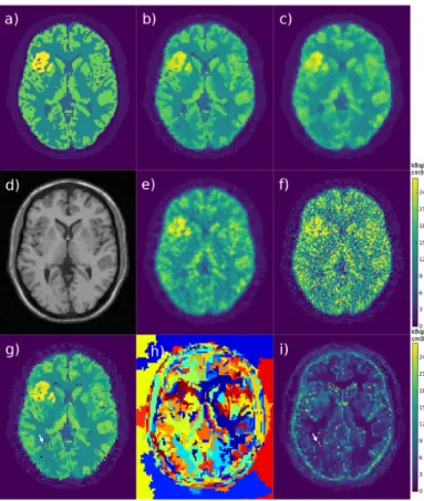
Fig.1 shows the simulated PET (Fig.1a) and MR (Fig.1d) images, the MLEM reconstruction without post-smoothing (Fig.1f) and with a post-smoothing matching the system res-olution (Fig.1e). The proposed method (Fig.1b) and the MR-MAP method (Fig.1c) are shown for near optimal parameter values that produced low estimator root mean square error and better visual image characteristics (sharper edges, but preserved PET unique features), α = 1 and β = 12.
In the proposed reconstruction, the edges are sharper than with other methods and overlap well with the edges in the true image, which can be interpreted as an improvement in spatial resolution. Some edges that do not exist in the MRI image are less visible in the reconstructed PET image,
Fig. 1. Simulation results for a single replicate: a) simulated PET image, b) RCP-GS mean, c) MR-MAP, d) simulated MR image, e) post-smoothed MLEM, f) converged MLEM, g) a sample of RCP-GS emission image, h) a sample of voxels clustering, i) RCP-GS 95% posterior intervals image; the MLEM colorscale in kBq/cm3 is common to all the PET emission images
for instance the lower edge of the lesion compared to the MR-MAP image. Image areas that have uniform intensity in the true image approach uniformity also in the proposed reconstruction, except for some individual voxels near strong edges which tend to have ’noisy’ artefacted values.
A sample of the PET emission image (Fig.1g) is shown along with the corresponding sample of voxels clustering (Fig.1h). Each cluster is composed of a certain amount of adjacent voxels. The clusters change in shape and size from sample to sample, and a single sample can contain both small and large clusters. When the hyperparameter α is increased, the overall spatial regularization is decreased, and the cluster size tends towards a single voxel, and vice versa.
In the image of 95% posterior intervals size (Fig.1i), areas with larger intervals tend to match areas in the reconstructed image where the intensities differ more from the true image, especially in the ’noisy’ artefacted voxels, which is promising regarding the diagnostic relevance of obtained uncertainty information. An example of noisy artefacted voxels is pointed out by a white arrow in the image sample (Fig.1g) and in the intervals image (Fig.1i), and by a black arrow in the clustering image (Fig.1h). They usually correspond to clusters containing a single or very few voxels, located near the edges of regions with different intensities.
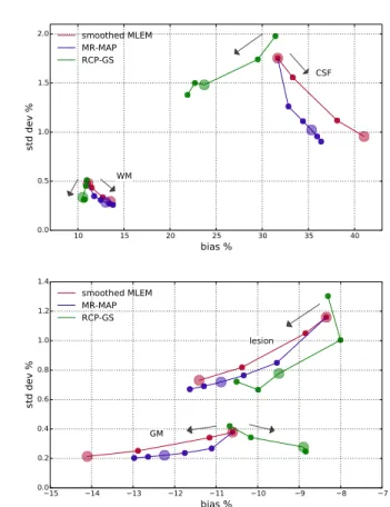
Fig.2 presents estimator (across replicates) bias - standard deviation plots for the selected regions of interest. For
hy-10 15 20 25 30 35 40 bias % 0.0 0.5 1.0 1.5 2.0 std dev % CSF WM smoothed MLEM MR-MAP RCP-GS 15 14 13 12 11 10 9 8 7 bias % 0.0 0.2 0.4 0.6 0.8 1.0 1.2 1.4 std dev % GM lesion smoothed MLEM MR-MAP RCP-GS
Fig. 2. Comparison of estimator bias - standard deviation for ROIs : larger dots correspond to images shown in Fig.1, and the arrows show the direction from lowest to highest spatial regularization)
perparameter values corresponding to images shown in Fig.1 (large dots in Fig.2), the proposed method presents lower bias compared to all the other methods for all the regions except for the lesion, for which the bias is higher than for converged MLEM (large red dot with lowest regularization) and lower than for the other methods, whereas the variance of the proposed method is lower compared to converged MLEM and higher compared to all the other methods. For all the methods, the hyperintense lesion and the gray matter are underestimated, and the CSF and WM are overestimated. For a fixed level of variance, the proposed method has the lowest bias for all the regions. The standard deviation percentage values are very low because large ROIs were selected (e.g. entire gray/white matter). The changes of bias values remain moderate.
Changing the strength of spatial regularization (based on both PET and MR data) in the proposed and in the MR-MAP method shows some similarities and some differences. For both methods, when the regularization strength is low, the estimator bias and variance tend to approach converged MLEM (large red dot with lowest regularization), and when the strength is high, the bias and variance tend to pull away from converged MLEM. For the proposed method, increasing the strength of regularization tends to lower both the bias and the variance, except in the lesion, where the bias tends to increase. For the MR-MAP method, increasing the strength tends to increase the bias and lower the variance. For the
proposed method, the tendency is not as strictly increasing or decreasing. It has been observed that for both the proposed and the MR-MAP method, increasing the strength of spatial regularization tends to cause the MR features to override slightly the PET features.
For hyperparameter values corresponding to images shown in Fig.1, the proposed method reduces the root mean square error of whole brain voxels by 66% compared to converged MLEM, by 36% compared to the MLEM with strongest post-smoothing, and by 22% compared to the MR-MAP.
The computation time for a single RCP-GS reconstruction was approximately 15min (30 runs × 1000 sampler iterations), compared to 22s for MR-MAP and 19s for MLEM (500 iterations). 20 10 0 10 20
spatial regularization [ log(α) ]
40 50 60 70 80 90 100
coverage of true value % GM
CSF WM lesion
Fig. 3. Simulated data: 95% posterior intervals’ coverage of true values for different values of RCP-GS hyperparameters (large dots correspond to the image shown in Fig.1b), for several ROIs; (lowest α = highest regularization)
The 95% posterior intervals are available only for the proposed method. Fig.3 presents for each ROI the percentage of ROI voxels for which the computed 95% posterior intervals include the true voxel intensity value (averaged over repli-cates), as a function of hyperparameter values (corresponding to different degrees of spatial regularization). As discussed in section II-C, this percentage should amount to 95% to be fully reliable, but it may drop when the models are not perfect (which is always the case to some extent with realistic data) and when estimators are biased. When the spatial regulariza-tion is low, the coverage of the posterior intervals approaches the required percentage, because the proposed method presents some bias and large variance (similar tendency as the con-verged MLEM), causing large intervals which are more likely to contain the true value in the presence of some bias. When the spatial regularization is high, the coverage drops, because the proposed method presents lower variance with still some bias (similar tendency as spatially penalized methods), causing tighter intervals that are less likely to contain the true value in the presence of bias. For near optimal hyperparameter values, corresponding to the image shown in Fig.1b, the percentage of whole brain voxels whose 95% posterior intervals contain the true value amounts to 70%, in average over replicates.
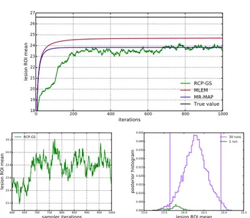
As mentioned in section II-C, the MCMC sampler iter-ations do not have the same meaning as MLEM or MAP optimization iterations. Fig.4(up) illustrates the evolution of the lesion ROI mean over iterations for RCP-GS (single
0 200 400 600 800 1000 iterations 18 19 20 21 22 23 24 25 26 27
lesion ROI mean RCP-GS
MLEM MR-MAP True value 600 650 700 750 800 850 900 950 1000 sampler iterations 23.2 23.4 23.6 23.8 24.0 24.2
lesion ROI mean
RCP-GS
23.0 23.5 24.0 24.5 25.0 25.5
lesion ROI mean
0.000 0.005 0.010 0.015 0.020 0.025 0.030 0.035 0.040 0.045 posterior histogram 30 runs 1 run
Fig. 4. Simulated data: (top) lesion ROI mean value over optimization iterations for MLEM and MR-MAP, and over sampler iterations for RCP-GS (single example run); (bottom left) the same single run RCP-RCP-GS curve zoomed to the last 400 samples and (bottom right) the posterior histograms of lesion ROI mean values, using the last 400 samples from the same single run (green) and from all the runs (violet, the vertical lines mark the bounds of the 95% posterior interval)
example run), MLEM and MR-MAP. Sampler iterations are different from optimization iterations in that the ROI mean is a random variable in this context: at each iteration, the computed value of the ROI mean represents a random sample from the posterior distribution, resulting in a randomly varying curve. The behaviour of RCP-GS sample curves, the imperfect mixing and the need for several runs of the sampler, are illustrated in detail in Fig.4(bottom). Fig.4(bottom left) shows the same single run RCP-GS curve zoomed to the last 400 samples: it can be observed that adjacent samples still show some correlation and explore the possible values relatively slowly. Fig.4(bottom right) shows the corresponding histogram (green), which represents only a partial contribution to the posterior histogram of the last 400 samples produced by all the runs (violet). The histogram for all the runs (violet) illustrates also the posterior distribution that can be obtained from the generated samples for the lesion ROI mean, with the corre-sponding 95% posterior interval bounds marked by vertical lines. The jump at iteration 100 for RCP-GS corresponds to the inclusion of the MR image, when the chosen α parameter becomes more appropriate (feature explained in section II-C). Sampler iterations are similar to optimization iterations in that the inverse problem is being solved: for MLEM the ROI mean tends towards a certain value, and for RCP-GS the ROI mean averaged over adjacent iterations (moving average) tends towards a certain value.
B. Patient data
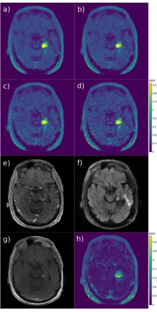
For the oncological 18F-FDG data set, a slice featuring the metastatic lesion in the brain stem is presented in Fig.5. The proposed reconstruction using both MR images (Fig.5h) presents sharper edges and more details compared to OSEM.
The lesion is sharper mostly thanks to the T1w MRI and some gray and white matter structures contain more details mostly thanks to the T2w MRI. The proposed and MR-MAP reconstructions using a single MR image show the influence of that image: the lesion edges become visually more similar to the edges in the MR image. The T1w MR image presents sharper depiction of the lesion, whereas the T2w MR image does not show much contrast in the lesion area. When using only the T1w MR image, lesion edges in the RCP-GS image (Fig.5f) are sharper and remain more consistent with the approximate edges in the OSEM image, compared to the MR-MAP image (Fig.5c). On the contrary, when using only the T2w MR image, lesion edges in the MR-MAP image (Fig.5d) are smoother and remain more similar to the approximate edges in the OSEM image, compared to the RCP-GS image (Fig.5g). The same 2D slice of a 3D sample of voxels clustering is also presented in Fig.5k: each color shade corresponds to a cluster label, containing only adjacent voxels. The clusters are smaller than actual anatomical or functional structures. The shape of clusters surrounding the head are caused by the mask applied during reconstruction for speed-up.
The computation time was 4 days for RCP-GS (30 runs × 250 sampler iterations), compared to 1h20 for MR-MAP and 50min for OSEM (8 iterations × 27 subsets).
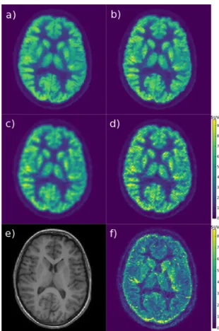
For the epilepsy18F-FDG data set, a slice featuring
struc-tures well delineated in PET and less delineated in MRI (thalamus, putamen, caudate nucleus, etc.) is presented in Fig.6. The proposed reconstruction (Fig.6a) presents sharper edges and more details, even in these central structures which are not well delimited in MR images. Small structures are better delineated than in the MR-MAP image (Fig.6b), and there is less noise, except for a couple of gray matter voxels which have a much higher intensity than they should. The image of posterior intervals (Fig.6f) presents larger intervals for these voxels with noisy artefacted intensities, and for the areas around some edges which are not visible in both images. For the glioma 18F-DOPA data set, a slice featuring the largest portion of the glioma is presented in Fig.7. The proposed reconstruction (Fig.7a) presents sharper edges, more details, and the lowest noise, in non pathological tissues and in the lesion. The lesion has different characteristics in different modalities. The proposed reconstruction is influenced by all the images, but the final shape remains approximately similar to the standard OSEM PET reconstruction (Fig.7c), though it is more round and smooth compared to OSEM and MR-MAP (Fig.7b). The image of posterior intervals (Fig.7h) presents larger intervals for some noisy artefacted voxels, for some areas whose edges are not visible in both modalities, and also for the lesion, especially near the edges.
V. DISCUSSION
The proposed method, RCP-GS, shows some interesting properties with respect to the MLEM/OSEM and to the MR-MAP method, in terms of bias and variance in the simulated data, and in terms of spatial regularization and influence of one or several MR images for both simulated and clinical data.
Fig. 5. Lesion exam: a) smoothed OSEM, b) OSEM, c) MR-MAP (T1w), d) MR-MAP (T2w), e) RCP-GS interval (both MR images), f) RCP-GS mean (T1w), g) RCP-GS mean (T2w), h) RCP-GS mean (both MR images), i) T1w MRI, j) T2w MRI, k) RCP-GS clustering sample; the OSEM colorscale in SUV is common to all the PET emission images
One of the main advantages of the proposed method is its ability to provide uncertainty information through the posterior distribution of the reconstructed image. Describing and presenting the posterior distribution of many correlated variables remains a challenge in statistics. These preliminary results summarize the posterior distribution through posterior intervals of individual voxels. Other features and represen-tations of the uncertainty and their applications remain to be explored in the future (e.g. posterior voxels covariance, statistical comparison of regions of interest). Further work is required to validate and characterize the resulting posterior dis-tribution and the derived uncertainty information, for instance by measuring the discrepancy and the fitness of the model with respect to the acquired data as in [27]. The uncertainty is propagated from several sources: from the prior distribution of intensity and spatial clustering, from observed PET data
Fig. 6. Epilepsy exam: a) RCP-GS mean, b) MR-MAP, c) post-smoothed OSEM, d) OSEM, e) T1w MRI, f) RCP-GS 95% posterior intervals; the OSEM colorscale in SUV is common to all the PET emission images
providing information about PET emission concentration and from observed PET and MRI data providing information about homogeneous regions. This is an interesting feature because it captures the complexity of the reconstruction process, but it also makes the interpretation of posterior intervals challeng-ing, because the various sources of uncertainty are difficult to separate. In Poisson and Gamma distributions, variance increases when the mean increases (this tendency has also been observed and explored theoretically in the context of standard MLEM [6]). Therefore, posterior intervals naturally tend to be wider in image regions with higher intensity. For the interpretation of PET images, it appears useful to analyze simultaneously an image of estimated emission concentration and the corresponding estimation uncertainty. Further work is needed for investigating more in depth the application of uncertainty information to diagnostic interpretation and diagnostic tasks.
This model was designed for standard patient acquisition protocols, so it is not intended for improving the reconstruc-tions of very noisy PET data. Further tests are required for evaluating the performances and the limits of the proposed method in terms of the SNR of PET raw data.
It should be noted that there is no final piece-wise clustering of the image: the grouping of voxels into homogeneous regions occurs only in individual samples of the posterior distribution, with clusters being usually much smaller than the actual anatomical or uniform areas in either image.
Fig. 7. Glioma exam: a) RCP-GS mean, b) MR-MAP, c) post-smoothed OSEM, d) OSEM, e) T1w MRI (Gd), f) FLAIR MRI, g) T1w late enhance-ment MRI (Gd), h) RCP-GS 95% posterior intervals; the OSEM colorscale in SUV is common to all the PET emission images
The ddCRP prior is more general and flexible than our current implementation. It models probabilistic grouping of voxels into spatial clusters with identical characteristics, which characteristics are arbitrary and independent of the clustering process. Here we chose a single simple characteristic, i.e. the cluster intensity, but more complex features could be used, in order to avoid the patchy aspect of individual image samples. Also, the distance weighting between voxels is here simply 1 for neighbour voxels and 0 for the others, but more complex weighting of distances between voxels could be tested, as in MAP methods. The ddCRP prior puts some assumptions on the overall average size of smooth regions and almost no assumption on regions intensity except the non-negativity. It should be noted that a deterministic method for solving inverse problems, such as MLEM, might also be viewed as a probabilistic method with a uniform (non-informative) prior. Further refinement of matching the statistical model to reality would imply using more accurate distributions, taking into
account the physics of the emission process and the complexity of the detection process that may be available in scanner raw data.
The lack of PET system resolution modeling in the recon-struction impairs slightly the matching of structures in MR and PET images. Hence, improvements are expected after the introduction of resolution modeling. As the backprojection is probabilistic in the proposed method, image convolution with system PSF cannot be used as easily as in conventional reconstructions. A solution consists in implementing the PSF directly into system matrix coefficients, but it is computa-tionally costly, even for usual reconstruction methods such as OSEM. Therefore, future work shall introduce PSF modeling in a probabilistic manner in the model.
Using Gaussian models for MRI processing or reconstruc-tion is common and widespread, even though the noise in MR magnitude images is best modeled with a Rayleigh distribu-tion. The model used here produced good initial results. As only the PET image is of interest here, sampling the posterior MRI cluster intensity is not relevant, but it could be done in order to obtain denoised MR images.
The computational load for MCMC methods is high, be-cause of the number of samples needed for converging to the actual posterior distribution and of the number of sam-ples needed afterwards for exploring thoroughly the space of possible unknown values and thus rendering accurately the posterior distribution. The Gibbs sampler’s mixing and conver-gence to the posterior distribution presented some difficulties, which is not a rare issue when applying MCMC samplers to realistic data and to models with many correlated random variables. In PET reconstruction inverse problem, the hidden variables (complete data n) imply high correlations, which tend to cause slower mixing and exploration of the domain of sample values. Our current solution to the mixing/convergence problem produces good results but remains empirical, and further work is needed for exploring more efficient and more theoretically sound solutions, as well as assessing the mixing properties more in depth, using methods described in [28]. When the sampler mixing improves, the number of iterations, the burn-in period, etc. shall be chosen in a less empirical way. There shall be no need for several runs, which should decrease the computation time. Convergence issues may show up especially in some very small or single-voxel clusters, whose intensity becomes trapped in inappropriate or ’noisy’ artefacted values. Small amount of backprojected counts per cluster, small cluster size and low cluster sensitivity increase the influence of the wide intensity prior, making the intensity of such clusters more difficult to sample.
The issue of potential detrimental influence of MRI on PET has to be addressed, as in MR-MAP methods. In the proposed method, the MR images do not affect the PET image intensity directly: they have an influence only on the clustering part of the model. The proposed and the MR-MAP method do not have the same approach to the spatial regularization and to the inclusion of side images, but there are some substantial similarities. Both methods have parameters that require tuning (1 free parameter for the proposed method and 4 for the MR-MAP method), and there is no universal automatic procedure
for choosing optimal parameters, especially for real data. In both methods, the spatial regularization depends on both PET and MRI, and the influence of parameter tuning shows similar trends: when parameters are tuned to increase the influence of MRI data, the shapes in the reconstructed PET image tend to fit the shapes in the MR image, regardless of whether they exist in the PET data or not. In the MR-MAP method, this issue occurs with strong smoothing penalty and strong reliance on MRI for the choice of neighbourhood voxels. In the proposed method, this issue occurs when allowing for larger clusters, especially when PET observed data are less reliable than MRI observed data, i.e. when MR images contain large homogeneous structures and have low noise, while the PET raw data have high noise level and contain inconsistencies. As far as differences between the methods are concerned, in the proposed method the MR image is neither a prior nor a part of the prior, contrary to usual MR-MAP methods. The MRI data are part of the observed noisy data that supply side information about smooth regions and structures. Including additional images requires also dealing with different voxel sizes and partial volume effects in PET and MRI data. Subsampling of MR images, mostly in axial direction, may impair the delineation of different tissues and create partial volume effects, while oversampling may create questionable structures, mostly when the spacing between 2D slices is large. Future work is needed to explore the behaviour of RCP-GS without the additional MR images, and to compare the spatial regularization performance to a MAP method based only on PET data.
To estimate a PET emission concentration image using posterior samples, it is easier and more reliable to estimate the posterior expectation than the posterior maximum, because of the quantity of available samples. The proposed estimator is thus optimal rather in the quadratic sense than in the maximum likelihood or maximum a posteriori sense.
VI. CONCLUSION
A new probabilistic PET reconstruction method named ”Random Clustering Prior - Gibbs Sampler” (RCP-GS) is presented, with the aim of reconstructing both a spatially regularized image and the associated uncertainty. This opens new areas for exploration and for applications. The proposed reconstruction showed appealing properties on both simulated and clinical data. Future work shall focus on improvements of sampler behaviour and on quantitative validation and interpre-tation of the estimated uncertainty.
ACKNOWLEDGMENT
The authors would like to thank Catherine Chiron (protocol EPIPED) and Micka¨el Soussan (protocol PROMISE) for pro-viding the clinical data, and Ma¨el Millardet for implementing penalized ML or MAP methods in CASToR. This work is supported by the Lidex-PIM project funded by the IDEX Paris-Saclay, ANR-11-IDEX-0003-02, by the ”MMIPROB” project funded by ITMO Cancer (France), and by the French national research agency (ANR-16-CE17-0011-001).
REFERENCES
[1] J. Qi and R. M. Leahy, “Iterative reconstruction techniques in emission computed tomography,” Physics in Medicine & Biology, vol. 51, pp. 541–578, 2006.
[2] B. Bai, Q. Li, and R. M. Leahy, “Magnetic resonance-guided positron emission tomography image reconstruction,” Seminars in Nuclear Medicine, vol. 43, no. 1, pp. 30–44, Jan. 2013.
[3] K. Vunckx, A. Atre, K. Baete, A. Reilhac, C. M. Deroose, K. V. Laere, and J. Nuyts, “Evaluation of three mri-based anatomical priors for quantitative pet brain imaging,” IEEE Transactions on Medical Imaging, vol. 31, no. 3, pp. 599–612, Mar. 2012.
[4] W. Hutchcroft, G. Wang, K. T. Chen, C. Catana, and J. Qi, “Anatomically-aided pet reconstruction using the kernel method,” Physics in Medicine & Biology, vol. 61, no. 18, p. 6668, 2016. [5] A. Mehranian, M. A. Belzunce, F. Niccolini, M. Politis, C. Prieto,
F. Turkheimer, A. Hammers, and A. J. Reader, “Pet image reconstruction using multi-parametric anato-functional priors,” Physics in Medicine & Biology, vol. 62, no. 15, p. 5975, 2017.
[6] H. H. Barrett, D. W. Wilson, and B. M. W. Tsui, “Noise properties of the em algorithm. i. theory,” Physics in Medicine & Biology, vol. 39, no. 5, p. 833, 1994.
[7] Y. Li, “Noise propagation for iterative penalized-likelihood image recon-struction based on fisher information,” Physics in Medicine & Biology, vol. 56, no. 4, p. 1083, 2011.
[8] S. Pedemonte, C. Catana, and K. V. Leemput, “Bayesian tomographic reconstruction using riemannian mcmc,” in Medical Image Computing and Computer-Assisted Intervention – MICCAI 2015. Springer Inter-national Publishing, 2015, pp. 619–626.
[9] A. Sitek, “Data analysis in emission tomography using emission-count posteriors,” Physics in Medicine & Biology, vol. 57, no. 21, p. 6779, 2012.
[10] S. Geman and D. Geman, “Stochastic relaxation, gibbs distributions, and the bayesian restoration of images,” IEEE Transactions on Pattern Analysis and Machine Intelligence, vol. PAMI-6, no. 6, pp. 721–741, Nov. 1984.
[11] I. S. Weir, “Fully bayesian reconstructions from single-photon emission computed tomography data,” Journal of the American Statistical Asso-ciation, vol. 92, no. 437, pp. 49–60, Dec. 1995.
[12] D. M. Higdon, J. E. Bowsher, V. E. Johnson, T. G. Turkington, D. R. Gilland, and R. J. Jaszczak, “Fully bayesian estimation of gibbs hyper-parameters for emission computed tomography data,” IEEE Transactions on Medical Imaging, vol. 16, no. 5, pp. 516–526, Oct. 1997. [13] E. Barat, C. Comtat, T. Dautremer, T. Montagu, and R. Trebossen, “A
nonparametric bayesian approach for pet reconstruction,” in 2007 IEEE Nuclear Science Symposium Conference Record, 2007, pp. 4155–4162. [14] M. D. Fall, E. Barat, C. Comtat, T. Dautremer, T. Montagu, and S. Stute, “Continuous space-time reconstruction in 4d pet,” in 2011 IEEE Nuclear Science Symposium Conference Record, Oct. 2011, pp. 2581–2586. [15] A. Sitek, “Reconstruction of emission tomography data using origin
ensembles,” IEEE Transactions on Medical Imaging, vol. 30, no. 4, pp. 946–956, Apr. 2011.
[16] D. M. Blei and P. I. Frazier, “Distance dependent chinese restaurant process,” Journal of Machine Learning Research, vol. 12, pp. 2461– 2488, 2011.
[17] S. Stute, C. Tauber, C. Leroy, M. Bottlaender, V. Brulon, and C. Comtat, “Analytical simulations of dynamic pet scans with realistic count rates properties,” in 2015 IEEE Nuclear Science Symposium and Medical Imaging Conference (NSS/MIC), Oct 2015, pp. 1–3.
[18] D. B. Rubin, “Bayesianly justifiable and relevant frequency calculations for the applies statistician,” The Annals of Statistics, vol. 12, no. 4, pp. 1151–1172, 1984.
[19] M. J. Bayarri and J. O. Berger, “The interplay of bayesian and frequentist analysis,” Statistical Science, vol. 19, no. 1, pp. 58–80, 2004. [20] T. Merlin, S. Stute, D. Benoit, J. Bert, T. Carlier, C. Comtat, M.
Fil-ipovic, F. Lamare, and D. Visvikis, “Castor: a generic data organization and processing code framework for multi-modal and multi-dimensional tomographic reconstruction,” Physics in Medicine & Biology, vol. 63, no. 18, p. 185005, 2018.
[21] (2017) Castor - customizable and advanced software for tomographic reconstruction. [Online]. Available: http://www.castor-project.org/ [22] H. Jeffreys, The Theory of Probability, 1961.
[23] J. Nuyts, D. Beque, P. Dupont, and L. Mortelmans, “A concave prior pe-nalizing relative differences for maximum-a-posteriori reconstruction in emission tomography,” IEEE Transactions on Nuclear Science, vol. 49, no. 1, pp. 56–60, Feb. 2002.
[24] J. E. Bowsher, H. Yuan, L. W. Hedlund, T. G. Turkington, G. Akabani, A. Badea, W. C. Kurylo, C. T. Wheeler, G. P. Cofer, M. W. Dewhirst, and G. A. Johnson, “Utilizing mri information to estimate f18-fdg distributions in rat flank tumors,” in IEEE Symposium Conference Record Nuclear Science 2004., vol. 4, Oct 2004, pp. 2488–2492.
[25] Brainweb: Simulated brain database. [Online]. Available: http://www.bic.mni.mcgill.ca/brainweb/
[26] D. L. Collins, A. P. Zijdenbos, V. Kollokian, J. G. Sled, N. J. Kabani, C. J. Holmes, and A. C. Evans, “Design and construction of a realistic digital brain phantom,” IEEE Transactions on Medical Imaging, vol. 17, no. 3, pp. 463–468, Jun. 1998.
[27] A. Gelman, X.-L. Meng, and H. Stern, “Posterior predictive assessment of model fitness via realized discrepancies,” Statistica Sinica, vol. 6, no. 4, pp. 733–760, 1996.
[28] N. Madras and A. D. Sokal, “The pivot algorithm: A highly efficient monte carlo method for the self-avoiding walk,” Journal of Statistical Physics, vol. 50, no. 1, pp. 109–186, Jan 1988.