HAL Id: halshs-01169268
https://halshs.archives-ouvertes.fr/halshs-01169268
Submitted on 29 Jun 2015
HAL is a multi-disciplinary open access
archive for the deposit and dissemination of sci-entific research documents, whether they are pub-lished or not. The documents may come from teaching and research institutions in France or
L’archive ouverte pluridisciplinaire HAL, est destinée au dépôt et à la diffusion de documents scientifiques de niveau recherche, publiés ou non, émanant des établissements d’enseignement et de recherche français ou étrangers, des laboratoires
Risk or Regulatory Capital? Bringing distributions back
in the foreground
Dominique Guegan, Bertrand Hassani
To cite this version:
Dominique Guegan, Bertrand Hassani. Risk or Regulatory Capital? Bringing distributions back in the foreground. 2015. �halshs-01169268�
Documents de Travail du
Centre d’Economie de la Sorbonne
Risk or Regulatory Capital?
Bringing distributions back in the foreground
Dominique G
UEGAN,Bertrand K. H
ASSANIRisk or Regulatory Capital?
Bringing distributions back in the foreground
May 22, 2015
• Dominique Guégan: Université Paris 1 Panthéon-Sorbonne, CES UMR 8174, 106 boule-vard de l’Hopital 75647 Paris Cedex 13, France, phone: +33144078298, e-mail: dguegan@univ-paris1.fr.
• Bertrand K. Hassani1: Grupo Santander and Université Paris 1 Panthéon-Sorbonne CES
UMR 8174, 106 boulevard de l’Hopital 75647 Paris Cedex 13, France, phone: +44 (0)2070860973, e-mail: bertrand.hassani@malix.univ-paris1.fr.
Abstract
This paper discusses the regulatory requirement (Basel Committee, ECB-SSM and EBA) to measure financial institutions’ major risks, for instance Market, Credit and Operational, regarding the choice of the risk measures, the choice of the distributions used to model them and the level of confidence. We highlight and illustrate the paradoxes and the issues observed implementing an approach over another and the inconsistencies between the methodologies suggested and the goal to achieve. This paper make some recommendations to the supervisor and proposes alternative procedures to measure the risks.2
Key words: Risk measures - Sub-additivity - Level of confidence - Extreme value distri-butions - Financial regulation
1
Disclaimer: The opinions, ideas and approaches expressed or presented are those of the authors and do not necessarily reflect Santander’s position. As a result, Santander cannot be held responsible for them.
2This paper has been written in a very particular period of time as most regulatory papers written in the past
20 years are currently being questioned by both practitioners and regulators themselves. Some distress or disarray has been observed among risk managers as most models required by the regulation were not consistent with their own objective of risk management. The enlightenment brought by this paper is based on an academic analysis of the issues engendered by some pieces of regulation and it has not for purpose to create any sort of polemic.
1
Introduction
The ECB-SSM3, the EBA4and the Basel Committee are currently reviewing the methodological framework of risk modelling. In this paper, we analyse some of the issues observed measuring the risks as prescribed that would be useful to address in the future regulatory documents.
1.1 Problematic
During the current crisis, the failure of models and the lack of capture of extreme exposures led regulators to change the way risks were measured either by requiring financial institutions to use particular families of distributions (Gaussian (BCBS (2005)), sub-exponantial (EBA (2014b))), either by changing the way dependencies were captured (EBA (2014b)) or suggesting switching from the VaR (Value-at-Risk)5 to sub-additive risk measures like the ES (Expected Shorfall)6 (BCBS (2013)). Indeed, risk modelling had played a major role during the crisis which began in 2008 either as catalysts or triggers. The latest changes proposed by the authorities have been motivated by the will to come closer to the reality of the financial markets.
Before capturing dependencies, the choice of the probability distributions used to model the risks and their associated measures are key points for practitioners and regulators. From a technical point of view, it is now accepted that the most relevant piece of information for risk managers is contained in the tails of the distributions characterising the risk factors they are willing to control. Thus it appears sensible that regulators, following theoretical and empirical studies and evolution of the risks associated to markets, financial products and actors behaviours adjust
3European Central Bank - Single Supervisor Mechanism 4European Banking Authority
5Given a confidence level p ∈ [0, 1], the VaR associated to a random variable X is given by the smallest number
x such that the probability that X exceeds x is not larger than (1 − p)
V aR(1−p)%= inf(x ∈ R : P (X > x) ≤ (1 − p)). (1.1)
6
For a given p in [0, 1], η the V aR(1−p)%, and X a random variable which represents losses during a prespecified
period (such as a day, a week, or some other chosen time period) then,
their requirements. Nevertheless analysing in details these requests, we note - inside the guide-lines - some confusions and misleading interpretations which cannot help to robustly evaluate and control these risks in financial institutions and also do not permit constructive exchanges between regulators and practitioners in order to reach the stability objective of the financial industry.
Thus, the purpose of this paper is to discuss some parts of the methodological framework pro-posed for risk modelling by the regulators and its evolution from 1995 to 2015, focusing on their strong incentive to use: (i) specific distributions to characterise the risks, (ii) specific risk measures, (iii) specific associated confidence level, and to apply these strategies independently from each others. We illustrate in the following that distributions, risk measures and confidence levels are three facets of a single object and are therefore indivisible. Thus, we argue that the approaches proposed by the regulators in the guidelines focusing on risk modelling engender a bias (positive or negative) in the computation of the risks, and consequently a distortion in the corresponding capital requirements, as soon as the problem of the measurement is not being dealt with in its globality.
Some of the following points are mainly addressed in this paper:
1. Is the choice of a particular risk measure ensures conservativeness?
2. What is the impact of the choice of a particular distribution on the associated risk measure?
3. For a single kind of risk: given a risk measure, what choice of the confidence level p is really appropriate?
4. When we use a V aRp measure, for which distributions is the sub-additivity7 property
fulfiled as soon as we consider several risk factors?
7
A coherent risk measure is a function ρ : L∞→ R:
• Monotonicity:If X1, X2∈ L and X1≤ X2 then ρ(X1) ≤ ρ(X2)
• Sub-additivity: If X1, X2∈ L then ρ(X1+ X2) ≤ ρ(X1) + ρ(X2)
• Positive homogeneity: If λ ≥ 0 and X ∈ L then ρ(λX) = λρ(X) • Translation invariance: ∀k ∈ R, ρ(X + k) = ρ(X) − k
5. Given that each risk type is modelled considering different distributions and using different
p-s, how can the sub-additivity criterion be fulfilled?
1.2 Questions raised by Regulatory proposals
For three categories of risks (market, credit8and operational), regulatory proposals regarding the choice of the distributions, the risk measures and the associated confidence level p are analysed. Issues related to their implementation have been highlighted in the following.
1.2.1 Market risks
1 - In the BCBS (1995) document, it is explicitly written:"The Committee has examined carefully how banks’ value-at-risk measures based on the parameters described above can be converted into a capital requirement that appropriately reflects the prudential concerns of supervisors. One of the problems of recognising banks’ value-at-risk measures as an appropriate capital charge is that the assessments are based on historical data and that, even under a 99% confidence inter-val, extreme market conditions are excluded. The Committee does not believe that a ten-day value-at-risk measure provides sufficient comfort for the measurement of capital for a number of reasons, which include: the past is not always a good guide to the future; the assumptions about statistical "normality" built into some models may not be justified, i.e. there may be "fat tails" in the distribution curve; the correlations assumed in the model may prove to be incorrect; market liquidity may become inadequate to close out positions.”
These proposals suggest several remarks concerning various very different concepts.
• First, the regulator says that the choice of the VaR as the risk measure excludes to take into account extreme events. This statement is not correct as the choice of the VaR is not the issue, it is the choice of the underlying distribution with which the associated quantile is evaluated that determines if the extreme events are captured or not. This question actually implied a second question about what is an extreme event as answering this question would suppose a complete information set.
• Second, the regulator discusses the inadequacy of using a "ten-day value at risk...." for the
8
measurement of the capital. Indeed, it is generally an error to use "the ten-day value at risk" but the reasons evoked by the regulators are sources of confusion. The errors found their origins in two main issues, the choice of the model by the practitioners (independence between the risk factors) on the first hand, and the implied Gaussian behaviour of the risk models, on the other hand. It would be more appropriate from a practical point of view to invite practitioners to work in a more robust way investigating both the properties and the patterns of their data: (i) Are they independent or not? (ii) Whatever the answer to this first question, what is the most appropriate model (according to adequacy, con-servativeness, or some other criteria)? (iii) How to capture the dependencies (not only between two risk factors using the concept of correlation which assumes also that there is some linearity between the risk factors, but a more general dependence architecture)? (iv) What is "the" distribution characterising the data set (it can be Gaussian, fat tailed, thin tailed, asymmetric, symmetric, multimodal etc....)? (v) How to justify the choice of the probability distribution they retain?
• Third, the question of the choice of the information set is crucial, but saying that the use of historical data is "not a good way to work" is particularly dangerous. Indeed, the historical data set is the only original information set available for the modeler. Concerning this information set, a more relevant question is to decide the period the modeler has to use and the length of this period. Thus, there is a huge mis-understanding from the regulator concerning the information set the practitioners have to use : "good" data sets do not exist.
• Fourth, when regulators said that modellers need to capture market liquidity with the information set, it was only rhetorical. As soon as a market is illiquid it creates a systemic risk which is another problem, consequently the question of the definition of liquidity risk should be raised. Why did the regulator introduce this issue in 1995? A debate is largely opened on the concept and even in 2015, to our knowledge, it does not emerge a "correct" and useful definition for this kind of risk in the literature, as the liquidity coverage ratio (LCR) supposed to evaluate the buffer covering the risk of being illiquid converges to zero as soon as the market tends to dry up. Note that we will not address this issue in the following as it is out of scope of this paper, but it was worth mentioning it with respect to the question of the data set quality.
2 - In Interpretive Issues with respect to the revisions to the market risk framework in November 2011, Page 8, paragraph 718 (xciii) (BCBS (2011b)) regarding the incremental risk capital, the Basel Committee stipulates that "in combination with the relevant rules on IRC, it is accepted that banks model issuer interdependence assuming multivariate normal distributions or normal copula (e.g. between asset values, credit spreads or default times) or must they show that such model assumptions do not underestimate risk?".
This proposal is surprising and very restrictive looking at the modelling of dependencies between the risk factors. Indeed the Gaussian copula takes the same information in both tails (it does not consider that asymmetry between information sets can exist). Furthermore, it does not consider the importance of fat tails, which is not consistent with the behaviour of most risks observed on financial markets (especially during the crisis). Since 2011, a lot of research using copula (like the Archimeadean copula for instance) and vines which take asymmetrical behavior and information in the tails has been conducted. This remark, is interesting as a Gaussian copula structure correspond to the inverse of a multivariate Gaussian distribution. We see that once again the world seems Gaussian regulatory speaking. We are quickly illustrating the issue below, though we will see that it is not helping addressing issues related to risk measures.
3 - Nevertheless the regulator in the same document states (page 9): "The onus is on the bank to justify the modelling choices and their impact to the national supervisor. Normal distributions or normal copula may not be assumed uncritically. The impact of such modelling choices must be analysed in the validation."
One may wonder why regulators propose so restrictive models (Gaussian framework in the pre-vious paragraph) to say after that they may not be good enough? Why not just giving the possibility to financial institutions to model the risk factors in the way they consider to be the best fit, and then rely on an independent validation process to validate their choice. 9
4 - In the Consultative Document concerning the Fundamental review of the trading book (BCBS (2013)) "A revised market risk framework", October 2013, Page 3, the Basel Committee proposes
9
to move from Value-at-Risk (VaR) to Expected Shortfall (ES) as "a number of weaknesses have been identified with using VaR for determining regulatory capital requirements, including its inability to capture “tail risk”". The ES measures the riskiness of a position by considering both the size and the likelihood of losses above a certain confidence level. The Committee has agreed to use a 97.5th ES for the internal models-based approach and has also used that approach to calibrate capital requirements under the revised market risk standardised approach.
With this more recent document it appears that the regulator thinks that the use of the ES instead of the VaR risk would permit to capture the most relevant information to measure the risks. This is not necessarily true as it still depends on the choice of the distributions used for the computation of this ES. Nevertheless, we know that this last measure is more interesting than the VaR as considering the same distribution it provides a better information concerning the amplitude of the risk, but if the fitted distribution is inappropriate the problem of capture of the extreme events remains the same. Besides, the choice of the level of confidence, for instance 97.5 is also arbitrary (this point has been illustrated in the next Section). Why does the regulator move from 99 % (in 1995) to 97,5 % (in 2012)? - Why do not they propose 95% or another value
p?.
1.2.2 Credit Risk and Counterparty Credit Risk
1 - In the International Convergence of Capital Measurement and Capital Standards, November 2005, Page 60 recommendation 71 (BCBS (2005)), the Basel Committee explicitly discusses the evaluation of the credit risk using an underlying Gaussian distribution along other parameters.
This proposal remains very limited and a dangerous approach, even if some robust works can be done when practitioners compute the probability of default (PD) (Guégan et al. (2013)), the loss given default (LGD) and the exposure of default (EAD). Using a Gaussian distribution even shifted considering the other parameters implies that the essence of the modelled risk has a Gaussian behaviour. Indeed, the intensity of default is transformed into a Gaussian quantile and somehow compared to the 99th percentile of the same Gaussian distribution. This is highly questionable and overly simplistic. What led to that conclusion? How is that possible to be backtested? This approach is nothing more than a transformed VaR. To the regulators’ credit
this model did not lead (yet) to massive failures, though low default portfolio credit risk mod-elling is currently being highly questioned.
Another issue that is worth mentioning but not dealt with in this paper is the independence between PD, LGD and EAD. This is not consitent with the piece of regulation requiering banks to capture wrong way risk, i.e. the upper tail dependence between PD and EAD (BCBS (2011a)).
2 - In the Article 383(4) of Regulation 575/2013 European Banking Authority - Consultation Paper - On Draft Regulatory Technical Standards (RTS) on credit valuation adjustment risk for the determination of a proxy spread and the specification of a limited number of smaller portfolios, and in the Article 383 of Regulation (EU) 575/2013 Capital Requirements Regula-tion - CRR, July 2013, Page 7 (EBA (2014a)), it is said "that instituRegula-tions are permitted (i) to use a VaR model for the measurement of specific market risk of debt instruments, (ii) to use an internal Expected Positive Exposure (EPE) model for the calculation of the exposure values to counterparty credit risk on the majority of their business, but use other methods (Mark-to-Market Method, Standardised Method or Original Exposures Method) for smaller portfolios".
It appears that these proposals are problematic as some "norms" are defined for banks internal models even if these models are totally inadequate when we fit them to real data. Nowhere regulators or experts from regulatory institutions provide the assumptions which justify the use of such models or such methodology. How can we interpret this absence of justifications? Is that a political decision? If the answer is yes, then what are the objectives? It seems to be the will of a "one size fits all" approach to be able to compare banks risk management performance. Unfortunately, if the model is inadequate, then the quality of the risk management will not be properly reflected and therefore the outcomes of the model misleading for both the authorities and the practitioners. Besides, it appears to be a bit despotic and to transfer the burden from the regulator onto the banks.
The credit value adjustment (CVA) is closely related to the evaluation of derivatives. The as-sumption is that models used to evaluate derivatives such as Black & Scholes as these models do not capture the risk of a counterparty defaulting. The CVA in its nature challenges the
use of Gaussian like distributions as it questions the soundness of the risk neutral valuation. Indeed the risk neutral valuation does not capture the risk of a counterparty to default, there-fore an adjustment has been created to add a buffer in capital. The expected positive exposure (EPE) used to evaluate the CVA is quite interesting too, as a symmetrical distribution such as the Gaussian distribution is used to capture an asymetric exposure (positive) (Gregory (2012)). This does not seem very sensible. It seems that once again, the regulation implies the use of a particular distribution even if it is not appropriate except maybe to simplify the calculations.
1.2.3 Operational risks
1 - In their article 312 of Regulation (EU) No 575/2013, June 2014, Page 43, the European Banking Authority - Consultation Paper - Draft Regulatory Technical Standards on assessment methodologies for the Advanced Measurement Approaches for operational risk (EBA (2014b)) states that "the competent authority shall verify that an institution pays particular attention to the positive skewness and leptokurtosis of the data when selecting a severity distribution. When the data are much dispersed in the tail, empirical curves shall not be used to estimate the tail region. Sub-exponential distributions shall be used for this purpose unless there exist exceptional reasons to apply other functions, which shall be in any case properly addressed and fully justified to prevent undue reduction of the capital figures." In Pages 17-18, "sub-exponential distributions" are defined as distributions whose right tail decreases slower than the exponential distribution. The class of sub-exponential distributions includes the lognormal, gamma, log-logistic, generalised Pareto, Burr, and Weibull (with shape parameter < 1) (Guégan and Hassani (2014)). The Weibull (with shape parameter > 1) and gamma distributions do not belong to the class of Sub-exponential distributions. Sub-exponential distributions can better represent the shape of the data in the tail (other than their skewness in the body) by allowing estimates of parameters that do not depend on the higher order statistical moments".
Comparing the proposal for operational risk modelling (Guégan and Hassani (2009), Guégan and Hassani (2013b)) with proposals to model other types of risks, we observe that for operational risks, experts thinking is ahead, however, some questions should be raised.
which is not specified, probably refers to the non-parametric fit which can be used, avoiding the price to pay with analytical forms. It is a pity not inciting practitioners to use this technique because it is well known by modelers that non-parametric fittings when they are correctly conducted, provides better fits than any parametric distributions and is generally used as a benchmark.
• Second, it is difficult to understand - from a parametric point of view - why the regulators focus on the limited list of distributions and why they consider them "at the same level" knowing that they have specific behaviors which cannot take into account all the features of the risks, and also knowing that the methodologies to fit them are so different. On the other hand, this list cannot be exhaustive as there exist other classes of distributions (quite common) useful to fit these kinds of risks and the regulatory paper does not make any reference to them assuming that a good fit would be found anyway using the distributions enumerated. The approach is in our opinion far too restrictive.
• As it seems that there is a mis-understanding regarding the foundation of their proposals concerning this list of distributions, we provide here an alternative and complementary approach for the choice of the distributions the modelers can use. If we consider the class of sub-exponential distributions and in particular those listed in the document we can say that from a probabilistic and statistical point of view, these distributions have very differ-ent properties. The generalised Pareto distribution belongs to the class of extreme value distribution and is fitted on data sets selected above a certain threshold. The Weibull distribution belongs to the class of extreme value distributions through the Theorem of Fisher-Tippett (Fisher and Tippett (1928)) appearing as the max -distribution for a cer-tain class of distributions. In practice we will fit this distribution on data sets built from the original data using block maxima method selecting the maxima inside the original data set. The other distributions, if they present any interest in risk modelling (what about the Burr distribution?) will be fitted on the whole sample. In fine, there is a lot of confusion for the choice of these distributions. It would be more interesting to introduce and classify correctly the classes of distributions they propose for their use in practice. Indeed, a large panel of classes of distributions can be considered: the Generalised Hyperbolic (GH) Class of distributions (Barndorff-Nielsen (1977)), the α-stable distributions (Samorodnitsky and
Taqqu (1994)), the g-and h distributions (Hoaglin (1985)) from one hand, and the extreme value distributions (Weibull, Fréchet, Gumbel), and the GPD distributions on the other hand. It is important to make a distinction between these two classes of distributions because the former ones are fitted on the whole sample and the latter ones on some spe-cific sub-samples which is fundamental in terms of risk management. Note also that the techniques of estimations differ for all these classes of distributions. Indeed, we use the whole sample (original data set) to estimate the GH, α-stable and g-and-h distributions, and maximum likelihood procedures will be used; Hill and Pickand methods are considered for estimating the parameters of the GPD distributions, and maximum likelihood method associated with block maxima methodology is used for the extreme value classes of dis-tributions. The choice of the distributions cannot be split from the difficulty to estimate its parameters and the underlying information set. For instance the GPD distribution is very difficult to fit on nearly all data set because of the estimation of the threshold which is a key parameter for this class of distributions and whose estimate is generally very unstable. An error in its estimation can create error, distortion and confusion on the allocation of the capital. It is surprising that the regulators do not take into account these issues before imposing such distributions. Their proposal is worthy of a Prévert setting but, unfortunately, does not correspond to a robust approach.
2 - In the same document (page 17, item 24), regulators discuss the choice of risk measure:"risk measure means a single statistic extracted from the aggregated loss distribution at the desired confidence level, such as Value at Risk (VaR), or shortfall measures (e.g. Expected Shortfall, Median Shortfall)".
This definition is particularly limitative. How the risk measures computed for different factors with different levels can be aggregated? Does the regulator has in mind the use of a spectral measure, then how can we use it? This would be interesting but the concept has never been discussed in any regulatory document. Thus, how robust is the method proposed?
1.3 To summarise
While these documents are addressing the main issues, we believe that some documents are too prescriptive, preventing banks from going beyond the proposals and focusing more on the
capital calculations than the risk management itself. Regarding the calculation of the capital requirement from the knowledge of the risk factors, the main points concerns the choice of the distribution, the choice of the risk measure and the choice of p. The regulator would like to impose some choices. In the previous subsection these ones and the strategies to evaluate the risks independently from each other are questioned. Consequently, in the following we discuss the distributions suggested in the regulatory documents to model the risks and we analyse the soundness of the risk measures and a priori confidence levels associated to these ones.
2
Alternative strategies to the regulatory papers
In the previous Section, the methodological choices implied by the regulation have been pre-sented and discussed, focusing on the nature of the distributions used to characterise a risk, the type of risk measure and the dependence structure to be applied. We point out some confusion and mis-understanding concerning the proposals of the regulators for these very technical points which are fundamental for the risk management of a banking institution as soon as these choices are determinant in the computation of the capital requirements, i.e. these should be risk sensi-tive. Thus, in this Section, using some data sets we illustrate and highlight the impact of these choices on practitioners10 perceptions of a risk.
2.1 Data set and strategy
We have selected a data set provided by a Tier European bank representing "Execution, Delivery and Process Management" risks from 2009 to 2013. "Execution, Delivery and Process Manage-ment" risk is a sub-category of operational risk. This data set is characterized by a distribution right skewed (positive skewness) and leptokurtic.
In order to follow regulators’ requirements in their different guidelines, we choose to fit on this data set some of the distributions proposed inside the regulatory documents and also others which seem more appropriate regarding the properties of the data set. We retain seven
tions. They are estimated (i) on the whole sample: the lognormal distribution (asymmetric and medium tailed), the Weibull distribution (asymmetric and thin tailed), a Generalised Hyperbolic (GH) distribution (symetric or asymmetric, fat tailed on an infinite support), an Alpha-Stable distribution (symmetric, fat tailed on an infinite support), a Generalised Extreme value (GEV) distribution (asymmetric and fat tailed), (ii) on an adequate subset: the Generalised Pareto (GPD) distribution (asymmetric, fat tailed) calibrated on a set built over a threshold, a Gener-alised Extreme value (GEVbm) distribution (asymmetric and fat tailed ) fitted using maxima coming from the original set. The whole data set contains 98082 data points, the sub-sample used to fit the GPD contains 2943 data points and the sub-sample used to fit the GEV using the block maxima approach contains 3924 data points. The objective of these choices is to evaluate the impact of the selected distributions on the risk representation, i.e. how the initial empirical exposures are captured and transformed by the model.
Table 1 exhibits parameters’ estimates for each distribution selected11. The parameters are esti-mated by maximum likelihood, except for the GPD which implied a POT (Guégan et al. (2011)) approach and the GEV fitted on the maxima of the data set (maxima obtained using a block maxima method (Gnedenko (1943))). The quality of the adjustment is measured using both the Kolmogorov-Smirnov and the Anderson-Darling tests. The results presented in Table 1 show that none of the distribution is adequate. This is usually the case when fitting unimodal distri-butions to multimodal data set. Indeed, multimodality of the distridistri-butions is a frequent issue modelling operational risks as the risk categories combine multiple kinds of incident, for instance, a category combining external fraud will contain the fraud card on the body, commercial paper fraud in the middle, cyber attack and Ponzi scheme in the tail. This comes back to an issue we have discussed previously, where empirical distributions would be more appropriate than fitted analytical distributions as it may help capturing multimodality. Unfortunately this solution has been crossed out by regulators as this solution is considered not being able to capture the tail properly. The use of fitted analytical distributions has been preferred despite the fact that sometimes no proper fit can be found and the combination of multiple distributions may lead to a high number of parameters and consequently to even more unstable results. Nevertheless
11In order not to overload the table the standard deviation of the parameters are not exhibited but are available
the question of multi-modality becomes more and more important concerning the fitting of any data set. In this paper we do not discuss this issue in more details as it is out of the scope of our objective as the regulators never suggest this approach: we provide some discussion on this methodological aspect of risk modelling in the conclusion (some references are for instance, Wang (2000) or Guégan and Hassani (2015a)).
Using this data set and the fit of the seven distributions, we compute for each distribution the associated VaRp and ESp for different values of p: the results are provided in Table 3. Then, in order to consider the question of sub-additivity and the competition between VaRp and ESp
when we have more than one risk factor we show the impact of the choice of the distributions on the computation respectively of the VaRp(X + Y ) and VaRp(X) + VaRp(Y ) where X and Y
are two risk factors. In this exercise, we compute the previous quantities in the following way:
• As VaRp(X) is a quantile, p ∈ [0, 1], we can build the whole spectrum of the VaR, i.e. the inverse of the cumulative distribution function. Summing VaRp(X) and VaRp(Y ) for each
value of p provides us with VaRp(X) + VaRp(Y ).
• To obtain VaRp(X +Y ), another approach is adopted. In a first step we randomly generate X and Y using the distribution fitted previously. Then X and Y are aggregated. The resulting cumulative distribution function is built and its inverse provide the spectrum of VaRp(X + Y ).
The results are provided in the Tables 4 to 15. We also illustrate these last results by graphes: they are given in Figures 1 to 7. We analyse now the results of these tables and Figures.
2.2 VaR
In this Section we analyse the results presented in Table 3 which provides the values obtained for the VaRp and the ESp computed from the seven distributions fitted on the data set or some
sub-samples, and also of Tables 4 to 15 which permit to address the property of non sub-additivity associated to the VaR. We also discuss figures 1 to 7 which illustrate this notion for the VaR, combining different distributions.
First and foremost, from Table 2, we can see that, p given, the choice of the distribution has a tremendous impact on the value of the risk measure, i.e. if a lognormal distribution is used, then the 99% VaR is equal to 3 039, while it is 22 for a Weibul adjusted on the same data and 84 522 using a GPD. A corollary is that the 90% VaR of the GPD is much higher than all the 99% VaR calculated with any other distribution. A first conclusion would be, what is the point of impos-ing a percentile if the practitioners are free to use any distribution (c.f. Operational Risk AMA)?
Second, given p, between the four distributions fitted on the whole sample (for instance lognor-mal, Weibull, GH and alpha-stable), compared to the GPD fitted above a threshold, we observe a huge difference for the VaR. A change in the threshold may either give higher or lower values depending, therefore the VaR is highly sensitive to the value of the threshold. Now, comparing the result obtained on the GEV fitted on the whole sample to the GEV fitted on the bock maxima, we observe the one focusing on the tails (GEV block maxima) leads to lower VaRs than a GEV capturing the entire set of information. Therefore, a more conservative information set associated to the appropriate distribution may lead to a lower VaR. The number of blocks considered may have some impact but nothing comparable to the effect of the threshold on a GPD. The Weibull which is a distribution contained in the GEV provides the lowest VaR.
Table 3 exhibits the risk measures obtained from fully correlated random variables. It is inter-esting to note that the risk measures obtained on fully correlated random variables and the sum of the risk measures obtained univariately are really similar. This means that as soon as we sum the VaR obtained on two variables we mechanically assume an upper tailed correlation for the random variables. Therefore, besides of being conservative the sum of univariate VaRs taken at the same level prevents the capture of any diversification benefit. Fully correlated random variables do not embed any diversification benefit by definition. Consequently, the analysis re-garding the sub-additivity of the risk measures have to be performed in another way.
So, as presented earlier, we randomly generated values from the distribution fitted before and combined them two by two. By way of this process we generated some random correlations and as a matter of fact some diversification. Then, we compared the risk measures obtained from the combination of random variables and the sum of the risk measures computed on the
random variables taken independently. Figures 1 to 5 represents the spectra of these two items and consequently allows comparing the risk measure obtained for different confidence levels. These figures show that depending on the combinations of distributions, the VaR may always be sub-additive, never sub-additive, only sub-additive in the tails, only sub-additive in the body or may be more erratic, i.e. can be sub-additive initially, then become non-sub-additive, and finally become sub-additive again in the tails. These observations are supported by Tables 12 to 14. Tables 14 also show the impact of the discretisation of the distributions on the risk measures, as this impact the sub-additivity. This last property is not only associated to the choice of the risk measure but definitively to the choice of the distribution and of the confidence level?
Analysing the results in details, we see in Table 4, for p fixed, that the VaR is never sub-additive if the lognormal distribution is associated to a GPD, while if the lognormal distribution is asso-ciated to any of the others, the VaR is usually sub-additive in the tails but not at the end of the body part. Note that if the lognormal is associated with an identical lognormal, the differences we have observed are only due to numerical errors related to the sampling. We expect the two values to be absolutely identical. Though, it is interesting to note that the random generation of numbers can be the root cause of non sub-additive results. Identical analysis can be done on other combinations (see table 6). Looking at Table 6 it appears that when the GPD has a positive location parameter, this prevents any combination from being sub-additive, because by construction the 0th percentile of the GPD is equal to the location parameter which should be according to Pickand’s theorem (Pickands (1975)), sufficiently high. At the 95th percentile, the VaR is always sub-additive as soon as a lognormal distribution is involved except if it is combined with a GPD. For the other distributions, it is not always true. For example, the VaR obtained combining a Weibull and a GEV fitted on the whole sample is not sub-additive. Table 7 shows that the use of an Alpha-Stable combined with any other distribution except the GPD provides sub-additive risk measures at the 99% level.
In Parallel, Figures 1 to 5 allows a more discriminating analysis of the behaviour of the compo-nent V aRp(X + Y ) versus V aRp(X) + V aRp(Y ). In Figure 1, we show that the sub-additivity
property is only verified for high percentile when we use a combination of a Weibull and a GH distributions, i.e. for p > 90%. Besides, the gap tends to enlarge as the percentiles increase.
Figure 2 exhibits a non sub-additive VaR from the 95th percentile, when we use the combi-nation of an Alpha-Stable distribution and a GEV fitted with the block maxima method, but the differences are not as large as on Figure 1. Figure 3 shows that combining two identical distributions does not always produce sub-additive risk measures though it should always be the case: this can be due to numerical errors engendered by the random generation of data points and the discretisation of the distribution. On Figure 4 and 5 we observe that the VaRs obtained from the combination of an Alpha-Stable distribution and a GH distribution or an Alpha-stable distribution and a GEV calibrated on maxima are never sub-additive below 70% . For com-parison purposes, Figures 6 and 7 illustrate that the combination of two elliptical distributions (respectively the Gaussian and the Student-t distributions) always leads to sub-additive VaRs.
2.3 Expected Shortfall
In this Section the results of the Table 3 are analysed. It provides the values obtained for the VaRp and the ESp computed from the seven distributions fitted on the data set or some sub-samples, and also of the Tables 4 to 15 which permit to verify the sub-addivity property of the ES risk measure.
The ES calculations are linked to the distribution used to model the underlying risks. Looking at Table 2, at the 95%, we observe that the ES goes from 18 for the Weibull to 216 127 for the GPD. Therefore, depending on the distribution used to model the same risk, at the same p level, the ES obtained is completely different. The corollary of that issue is that the ES obtained for a given distribution at a lower percentile will be higher than the ES computed on another distribution at a higher percentile. For example, Table 2 show that the 90% ES obtained from an Alpha-Stable distribution is much higher than the 99.9% ES computed on a lognormal dis-tribution.
The comments regarding the impact of the choice of the information sets on the calculation of the considered risk measure are identical to those stated in the third paragraph of the previous section except regarding 2 points. First, results obtained from the GPD and the alpha-stable distribution are of the same order. Second, the differences between the GPD and the GEV fitted on the block maxima are huge, illustrating the fact that despite being two extreme value
distributions, the information captured is quite different.
Regarding the sub-additivity issue, by building the ES always lead to sub-additive values, con-trary to the VaR for which this property is not always verified and depends on the underlying distribution. It is interesting to note that if we combine two ES taken at two different levels of confidence p, the ES may not be sub-additive anymore. This is a point that the regulator does not discuss when he says that we have to aggregate the risk measures. This issue is particu-larly important for risk managers, as soon as the level of confidence prescribed in the regulation guidelines is different from a risk factor to another and appears totally arbitrary.
While the use of several confidence levels pi, i = 1, · · · , k allowing to have a spectral
represen-tation of the risk measure (VaR or ES) could be interesting but the approach proposed by the regulator which mixes distribution and confidence level is questionable. Indeed, the 70% ES of some combinations may lead to much higher value that the 99.9th (Table 9, WE-GPD vs WE-GH).
2.4 VaR vs Expected Shortfall
Previously we illustrate the fact that, depending on the distribution used and the confidence level chosen, the values provided by VaRp can be bigger than the values derived for an ESp and
conversely. Thus a question arises: What should we use the VaR or the Expected Shortfall? To answer to this question we can consider several points:
• Conservativeness: Regarding that point, the choice of the risk measure is only relevant for a given distribution, i.e. for any given distribution the VaRp will always be inferior to the ESp (assuming only positive values) for a given p. But, if the distribution used to
characterise the risk is to be chosen and fitted, then it may happen that for a given level
p, the VaRp obtained from a distribution is superior to the ESp. For example Table 2
shows that the 99.9% VaR obtained using the GEV distribution fitted with block maxima is superior to the ES obtained for any other distribution at the same level p.
• Sub-additivity: In that case only the expected shortfall guarantees always the sub-additivity of the measure as soon as the p is set, but for some distributions the VaR can be also
sub-additive.
• Distribution and p impacts: Table 2 shows that potentially a 90% level ES obtained on a given distribution is larger than a 99.9% VaR obtained on another distribution, e.g. the ES obtained from a GH distribution at 90% is higher that the VaR obtained form a lognormal distribution at 97.5%. Thus is it always pertinent to use a high value for p?
• Parameterisation and estimation: the impact of the calibration of the estimates of the parameters is not negligible (Guégan et al. (2011)), mainly when we fit a GPD. Indeed in that latter case, due to the instability of the estimates for the threshold, the practitioners can largely overfit the risks. Thus, why the regulators still impose this distribution?
3
Conclusion and Recommendations
In the introduction, analysing several guidelines issued by the EBA and the Basel Committee, we pointed out the fact that the regulators impose specific distributions, risk measures and con-fidence levels to analyse the risk factors in order to evaluate the capital requirements of financial institutions. It appears that their approach is non holistic and their analysis of the risks relies on a disconnection between the choice of the distributions, the risk measures and the confidence level, tools necessary for risks assessments.
In this paper we show that the risk measurement for financial institutions depends intrinsically on how the tools are chosen, i.e. the distribution, the combinations of these distributions, the type of risk measure and the level of confidence. Therefore, the existence of a risk measure as discussed in the regulation is questionable, as for example modifying the level of confidence by a few percents would result in completely different interpretations. The regulators fail to propose an appropriate approach to measure these risks in financial institutions as soon as they do not take into account the problem of risk modelling in its globality.
Regulators are by far too prescriptive and their choices questionable:
• Imposing distributions makes no sense whatever the risks to be modeled. Where are these a priori coming from?
• The regulation reflect some misunderstanding of distributions’ properties (probabilist ap-proach) and of the particular properties surrounding their fitting (statistical apap-proach).
• The levels of confidence p seems rather arbitrary. They neither take into account the flexibility of risk measures nor the impact of the underlying distribution, misleading risk managers.
While these fundamental problems are not addressed, others are completely ignored such as the concept of spectral analysis, or of distortion risk measures (Sereda et al. (2010), Guégan and Hassani (2015a)). Despite the cosmetic changes included in Basel II and III, the propositions do not enable a better risk management, and banks response to regulatory points are not ap-propriate as they do not correspond to the reality. It is therefore not surprising that capital calculations and stress testing are still unclear, and that these are not able to capture asymmet-ric chocs corresponding an extreme incident (black swan, dinosaur or dragon).
Some other questions should also be addressed:
• Is that more efficient in terms of risk management to measure the risk and then build a capital buffer or to adjust the risk taken considering the capital we have? In other word, maybe should banks start optimising their income generation with respect to the capital they already have.
• The previous points are all based on unimodal parametric distributions to characterise each risk factor, what is the impact of using multimodal distributions in terms of risk measurement and management? We believe that an empirical evaluation of the risk pro-vides bank with a reliable benchmark and a starting point in term of what would be an acceptable capital charge or risk assessment.
• One of the biggest issue lies in the fact that we do not know how to combine or aggregate
V aR(X)p1, V aR(Y )p2 and V aR(Z)p3 evaluated on three different kinds of risks at three
different confidence level p1, p2, p3. This mechanically prevents banks from building a
holistic approach from a capital point of view. How should we proceed to solve the problem, should we use p = max(p1, p2, p3), or the min or the average?
• While in this paper we focused on each factor taken independently, the question of the dependence is quite important too. Maybe not as important as the impact of the distri-bution selected for the risk factor (Guégan and Hassani (2013a)) but non addressing this issue properly could lead to a mis-interpretation of the results. The choice of the copula has a direct impact on the dependence structure we would like to apply and the capture of shocks. For instance, a Gaussian or Student t-copula is symmetric, despite the fact that a t-copula with a low number of degrees of freedom could capture tail dependencies, these would not capture asymmetric shocks. Archimedean or Extrema Value copulas associated to a vines strategy would be more appropriate (Guégan and Maugis (2010)).
• In a situation such as depicted by a stress-testing process with forward looking perspective, if the risks are not correctly measured then the foundations will be very fragile and the outcome of the exercise not reliable. Indeed, stressing a situation requires an appropriate initial assessment of the real exposure, otherwise the stress would merely model what should have been captured originally and therefore be useless (Bensoussan et al. (2015), Guégan and Hassani (2015b), Hassani (2015)).
We came up to the conclusion that the debate related to the selection of a risk measure over another is not really relevant, and considering issues raised in the previous sections our main recommendation would be to leave as much flexibility as possible to the modellers to build the most appropriate models for risk management purposes initially and then extended with conservative buffers for capital purposes. The idea would be to bring the idea that a good risk management would mechanically limit the exposure and the losses and therefore ultimately reduce the regulatory capital burden. Models should only be a reflexion of the underlying risk framework and not a tool to justify a reduced capital charge. We would like to see more the supervisory face of the authorities and less their regulatory one, in other words we would like them to stop focusing so much on banks risk measurement comparability and more on financial institutions risk understanding. It would probably be wise if both regulators and risk managers were working together (e.g., academic formation open to both corpus, regular workshops, etc., (Guégan (2009))) instead as opponents in order to reach their objective of stability of the financial system for the first and profitability for the second.
References
Barndorff-Nielsen, O. (1977), ‘Exponentially decreasing distributions for the logarithm of par-ticle size’, Proceedings of the Royal Society of London. Series A, Mathematical and Physical
Sciences (The Royal Society) 353 (1674), 401–409.
BCBS (1995), ‘An internal model-based approach to market risk capital requirements’, Basel
Committee for Banking Supervision, Basel .
BCBS (2005), ‘International convergence of capital measurement and capital standards - a re-vised framework’, Basel Committee for Banking Supervision, Basel .
BCBS (2011a), ‘Basel iii: A global regulatory framework for more resilient banks and banking systems’, Basel Committee for Banking Supervision, Basel .
BCBS (2011b), ‘Interpretative issues with respect to the revisions to the market risk framework’,
Basel Committee for Banking Supervision, Basel .
BCBS (2013), ‘Fundamental review of the trading book: A revised market risk framework’,
Basel Committee for Banking Supervision, Basel .
Bensoussan, A., Guégan, D. and Tapiro, C., eds (2015), Future Perspectives in Risk Models and
Finance, Springer Verlag, New York, USA.
EBA (2014a), ‘Consultation paper- on draft regulatory technical standards (rts) on credit val-uation adjustment risk for the determination of a proxy spread and the specification of a limited number of smaller portfolios and in the article 383 of regulation (eu) 575/2013 capital requirements regulation - crr’, European Banking Authority, London .
EBA (2014b), ‘Draft regulatory technical standards on assessment methodologies for the ad-vanced measurement approaches for operational risk under article 312 of regulation (eu) no 575/2013’, European Banking Authority, London .
Fisher, R. A. and Tippett, L. H. C. (1928), ‘Limiting forms of frequency distributions of the largest or smallest member of a sample’, Proc. Cambridge Philosophical Soc. 24, 180 – 190.
Gnedenko, B. (1943), ‘Sur la distribution limite du terme d’une série aléatoire’, Ann. Math.
Gregory, J. (2012), Counterparty Credit Risk and Credit Value Adjustment: A Continuing
Chal-lenge for Global Financial Markets, 2nd Edition edition, John Wiley & Sons, London.
Guégan, D. (2009), Former les analystes et les opérateurs financiers, in G. Giraud and C. Re-nouard, eds, ‘20 propositions pour réformer le capitalisme’, Flammarion, Paris, France.
Guégan, D. and Hassani, B. (2009), ‘A modified panjer algorithm for operational risk capital computation’, The Journal of Operational Risk 4, 53 – 72.
Guégan, D. and Hassani, B. (2013a), ‘Multivariate vars for operational risk capital computation : a vine structure approach.’, International Journal of Risk Assessment and Management
(IJRAM) 17(2), 148–170.
Guégan, D. and Hassani, B. (2013b), ‘Using a time series approach to correct serial correlation in operational risk capital calculation’, The Journal of Operational Risk 8(3), 31–56.
Guégan, D. and Hassani, B. (2014), ‘A mathematical resurgence of risk management: an extreme modeling of expert opinions.’, Frontiers in Economics and Finance pp. 25–45.
Guégan, D. and Hassani, B. (2015a), Distortion risk measures or the transformation of unimodal distributions into multimodal functions, in A. Bensoussan, D. Guégan and C. Tapiro, eds, ‘Future Perspectives in Risk Models and Finance’, Springer Verlag, New York, USA.
Guégan, D. and Hassani, B. (2015b), Stress testing engineering: the real risk measurement?,
in A. Bensoussan, D. Guégan and C. Tapiro, eds, ‘Future Perspectives in Risk Models and
Finance’, Springer Verlag, New York, USA.
Guégan, D., Hassani, B. and Naud, C. (2011), ‘An efficient threshold choice for the computation of operational risk capital.’, The Journal of Operational Risk 6(4), 3–19.
Guégan, D., Hassani, B. and Zhao, X. (2013), Emerging countries sovereign rating adjust-ment using market information: Impact on financial institutions investadjust-ment decisions, in M. El Hedi Arouri, S. Boubaker and D. Nguyen, eds, ‘Emerging Markets and the Global Economy: A Handbook’, Academic Press, Oxford.
Guégan, D. and Maugis, P.-A. (2010), ‘New prospects on vines.’, Insurance Markets and
Hassani, B. (2015), ‘Risk appetite in practice: Vulgaris mathematica’, The IUP Journal of
Financial Risk Management 12(1), 7–22.
Hoaglin, D. C. (1985), ‘Summarizing shape numerically: the g-and-h distributions’, John Wiley
& Sons pp. 461–513.
Pickands, J. (1975), ‘Statistical inference using extreme order statistics’, annals of Statistics
3, 119–131.
Samorodnitsky, G. and Taqqu, M. (1994), Stable Non-Gaussian Random Processes: Stochastic
Models with Infinite Variance, Chapman and Hall, New York.
Sereda, E., Bronshtein, E., Rachev, S., Fabozzi, F., Sun, W. and Stoyanov, S. (2010), Dis-tortion risk measures in portfolio optimisation, in J. Guerard, ed., ‘Handbook of Portfolio Construction’, Volume 3 of Business and Economics, Springer US, pp. 649–673.
Wang, S. S. (2000), ‘A class of distortion operators for pricing financial and insurance risks.’,
1 2 3 4 5 6 7 0 5000 10000 15000 20000 25000 30000
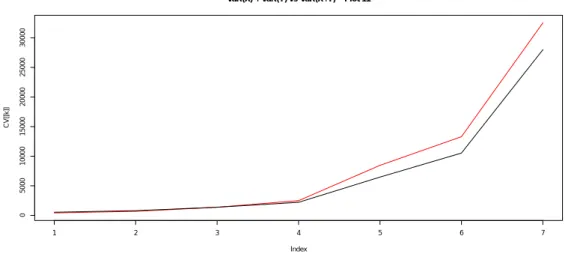
VaR(X) + VaR(Y) vs VaR(X+Y) − Plot 11
Index
CV[[k]]
Figure 1: This plot represents the sum of VaR(X) and VaR(Y) (red) versus VaR(X + Y) (black). The random variable X has been generated using a Weibull distribution and Y has been obtained from a Generalised Hyberbolic distribution. The percentiles represented are the 70th, 80th, 90th, 95th, 99th, 99.5th and 99.9th. For high percentiles, the VaR seems to be sub-additive.
1 2 3 4 5 6 7
0
50000
100000
150000
VaR(X) + VaR(Y) vs VaR(X+Y) − Plot 35
Index
CV[[k]]
Figure 2: This plot represents the sum of VaR(X) and VaR(Y) (red) versus VaR(X + Y) (black). The random variable X has been generated using a Alpha-stable distribution and Y has been obtained from a GEV distribution calibrated on maxima. The percentile represented are the 70th, 80th, 90th, 95th, 99th, 99.5th and 99.9th. For high percentiles, the VaR is not sub-additive.
1 2 3 4 5 6 7 0 20000 40000 60000 80000
VaR(X) + VaR(Y) vs VaR(X+Y) − Plot 43
Index
CV[[k]]
Figure 3: This plot represents the sum of VaR(X) and VaR(Y) (red) versus VaR(X + Y) (black). The random variables X and Y have been obtained from two identical GEV distributions. The percentiles represented are the 70th, 80th, 90th, 95th, 99th, 99.5th and 99.9th. For high per-centiles, the VaR is sub-additive.
0 10 20 30 40 50 60 0 5000 10000 15000 20000 25000
VaR(X) + VaR(Y) vs VaR(X+Y) − Plot 34
Index
CV[[k]]
Figure 4: This plot represents the sum of VaR(X) and VaR(Y) (red) versus VaR(X + Y) (black). The random variable X has been generated using a Alpha-stable distribution and Y has been obtained from a Generalised Hyperbolic distribution. The percentiles represented are sequentially going from the 10th to the 70th with a step of 1% between two points. The VaR represented are never sub-additive.
0 10 20 30 40 50 60 50 100 150 200 250 300 350
VaR(X) + VaR(Y) vs VaR(X+Y) − Plot 35
Index
CV[[k]]
Figure 5: This plot represents the sum of VaR(X) and VaR(Y) (red) versus VaR(X + Y) (black). The random variable X has been generated using a Alpha-stable distribution and Y has been obtained from a GEV distribution calibrated on maxima. The percentiles represented are sequentially going from the 10th to the 70th with a step of 1% between two points. The VaR represented are never sub-additive.
● ● ●● ●●● ● ● ●● ● ● ●● ●● ● ● ●● ●● ● ●● ● ● ● ● ●● ● ●● ● ●● ● ●● ● ● ● ● ●● ● ●● ● ●● ● ● ● ● ●● ● ●● ● ●● ● ●● ● ● ● ● ●● ● ● ● ● ●● ● ● ●● ●● ● ● ●● ● ●●●● ●● ● ● ● 0 20 40 60 80 100 −2 0 2 4 6 8 10 Gaussian illustration Index dd
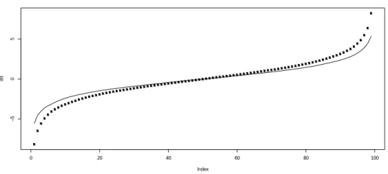
Figure 6: This plot represents the sum of VaR(X) and VaR(Y) (doted line) versus VaR(X + Y) (solid line). The random variable X has been generated using a Gaussian distribution (0, 1) and Y has been obtained from a Gaussian distribution (2, 1). The VaRs represented are always sub-additive.
● ● ● ● ● ●● ●● ●● ● ● ●● ● ● ●● ● ● ● ●● ● ● ● ● ●● ● ●● ● ● ● ● ● ●● ● ● ●● ● ● ● ● ● ● ●● ● ● ●● ● ● ● ● ● ●● ● ●● ● ●● ● ● ● ● ●● ● ●● ● ● ●● ●● ● ● ●● ● ●●● ●● ● ● ● ● ● 0 20 40 60 80 100 −5 0 5
Student t−distribution illustration
Index
dd
Figure 7: This plot represents the sum of VaR(X) and VaR(Y) (doted line) versus VaR(X + Y) (solid line). The random variable X has been generated using a Student-t distribution (3 df) and Y has been obtained from a Student-t distribution (4 df). The VaRs represented are always sub-additive.
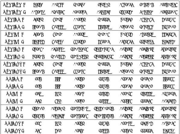
P arameters Distribution LogNormal W eibull GPD GH Alpha-Stable GEV GEV BM µ 4.412992 -1541.558 -5.5846599 -587.855749 50.272385 σ 1.653022 -2137.940297 64.720971 p -0.5895611 -0.1906536 0.86700 -β -182.9008432 1185.8083087 0.1906304 0.95000 -ξ -0.9039617 -675 923 3.634536 1.030459 δ -22.5118547 58.18019 -λ --0.871847 -γ -54.21489 -KS < 2.2e-16 < 2.2e-16 < 2.2e-16 < 2.2e-16 < 2.2e-16 < 2.2e-16 < 2.2e-16 AD 6.117e-09 6.117e-09 6.117e-09 NA 6.117e-09 (d) 6.117e-09 6.117e-09 T able 1: Distribution P arameters -This table presen ts the parameters obtain for the mo del. The p-v alues of b oth K olmogoro v-Smirno v and Anderson -Darl in g tests are also pro vided.
%tile Distribution LogNormal W eibull GPD GH Alpha-Stable GEV GEV BM V aR ES V aR ES V aR ES V aR ES V aR ES V aR ES V aR ES 90% 686 2075 7 13 10 745 142 444 624 2 927 582 50 323 2 097 291 3.072299e+19 626 8 755 95% 1251 3237 11 18 19 906 216 127 1 307 4 961 1 209 99 827 28 699 710 6.144597e+19 1 328 16 617 97 .5% 2107 4875 15 23 37 048 351 202 2 601 8 100 2 563 197 937 373 552 400 1.228919e+20 2 762 31 362 99% 3860 8039 22 31 84 522 715 347 5 916 14 522 7 105 488 689 1.073230e10 3.072299e+20 7 177 71 949 99 .9% 13646 24435 44 55 675 923 4 893 789 26 435 44 727 98 341 4 691 025 4.702884e+13 3.072299e+21 77 463 550 299 T able 2: Univ ariate Risk Measures -This table e xh ibits the V aRs and ESs for the sev en typ es of distributions considered for fiv e confidence lev el (for instance, 90%, 95%, 97.5%, 99% and 99.9%)
X1 X2 LogNormal W eibull GPD GH Alpha-Stable GEV GEV BM V aR X1 ,X 2 E SX 1 ,X 2 V aR X1 ,X 2 E SX 1 ,X 2 V aR X1 ,X 2 E SX 1 ,X 2 V aR X1 ,X 2 E SX 1 ,X 2 V aR X1 ,X 2 E SX 1 ,X 2 V aR X1 ,X 2 E SX 1 ,X 2 V aR X1 ,X 2 E SX 1 ,X 2 LogNormal p1 2 493 6 103 2 328 4 820 75 546 217 916 2 618 7 753 2 552 44 407 2.834332e+07 1.721696e+21 2 658 19 225 p2 4 087 9 057 3 528 6 805 93 442 353 270 4 662 12 064 4 731 85 397 3.665483e+08 3.443392e+21 4 872 34 914 p3 7 252 14 693 5 735 10 419 142 038 716 560 9 291 20 539 10 725 203 193 1.072611e+10 8.608479e+21 10 723 76 829 p4 24 250 43 132 16 710 27 468 746 560 4 871 970 36 925 59 361 111 991 1 789 756 5.390204e+13 8.608479e+22 83 960 551 875 W eibull p1 -2 230 3 637 75 270 219 140 2 424 6 507 2 345 80 360 2.874992e+07 1.648438e+21 2 459 32 126 p2 -3 110 4 663 92 818 356 117 4 019 9 939 4 029 157 714 3.746901e+08 3.296876e+21 4 202 61 102 p3 -4 425 6 176 140 307 725 572 7 651 16 774 9 003 385 667 1.062522e+10 8.242191e+21 8 856 143 962 p4 -8 542 10 777 744 266 4 982 719 29 929 48 745 102 987 3 644 010 4.051415e+13 8.242191e+22 81 979 1 249 637 GPD p1 -150 276 481 590 75 882 198 596 76 003 253 293 2.900050e+07 8.175899e+21 2.852749e+07 8.991075e+20 p2 -185 210 799 161 93 953 314 173 94 929 423 142 3.804500e+08 1.635180e+22 3.719388e+08 1.798215e+21 p3 -281 725 1 667 960 143 016 618 297 149 135 886523 1.055955e+10 4.087950e+22 1.038451e+10 4.495538e+21 p4 -1 482 342 12 136 572 735 168 3 911 547 869 960 6 369 873 5.299107e+13 4.087950e+23 4.773943e+13 4.495538e+22 GH p1 -2 784 9 385 2 705 73 357 2.880134e+07 3.149731e+20 2.875817e+07 6.426626e+19 p2 -5 338 14 981 5 470 142 939 3.771517e+08 6.299462e+20 3.674012e+08 1.285325e+20 p3 -11 469 25 984 13 280 344 980 1.092553e+10 1.574866e+21 1.088133e+10 3.213313e+20 p4 -47 282 75 037 120 486 3 167 054 5.156340e+13 1.574866e+22 4.991674e+13 3.213313e+21 Alpha-Stable p1 -2 649 146 535 2.868921e+07 2.877576e+22 2 822 31 932 p2 -5 648 289 288 3.667449e+08 5.755152e+22 5 644 59 930 p3 -15 890 709 490 1.007457e+10 1.438788e+23 13 339 137 177 p4 -225 543 6 659 012 3.907140e+13 1.438788e+24 96 356 1 107 042 GEV p1 -1.822300e+08 1.096423e+28 2.875582e+07 1.635820e+19 p2 -2.615063e+09 2.192846e+28 3.640431e+08 3.271639e+19 p3 -8.028848e+10 5.482116e+28 1.075443e+10 8.179098e+19 p4 -4.437624e+14 5.482116e+29 4.820065e+13 8.179098e+20 GEV BM p1 -2 894 59 150 p2 -5 985 114 221 p3 -15 597 271 596 p4 -170 339 2 336 019 T able 3: Correlated Risk Measures -this table presen ts the V aRs and the ESs obtained on fully correlated random v ariables.
LN-LN 1 393 663 1, 373 2, 503 7, 721 11, 661 27, 292 LN-LN 2 395 667 1, 376 2, 503 7, 721 11, 677 27, 517 LN-WE 1 447 742 1, 439 2, 427 6, 299 8, 924 18, 498 LN-WE 2 564 826 1, 374 2, 068 4, 654 6, 406 14, 066 LN-GPD 1 4, 321 6, 181 11, 432 21, 158 88, 382 163, 788 689, 569 LN-GPD 2 58, 968 60, 766 65, 759 74, 945 138, 510 209, 859 726, 643 LN-GH 1 364 611 1, 313 2, 569 9, 882 16, 037 41, 329 LN-GH 2 480 742 1, 418 2, 528 8, 205 12, 765 30, 592 LN-AS 1 377 614 1, 269 2, 461 10, 965 21, 402 111, 987 LN-AS 2 476 725 1, 374 2, 472 9, 657 18, 319 101, 929 LN-GV 1 25, 132 137, 464 2, 097, 977 28, 700, 959 10.73e9 134.51e9 47, 029e9 LN-GV 2 25, 313 138, 221 2, 095, 098 29, 156, 891 10.47e9 135.38e9 45, 501e9 LN-GVb 1 366 614 1, 312 2, 579 11, 037 20, 542 91, 109 LN-GVb 2 481 742 1, 423 2, 571 9, 670 17, 603 80, 694
Table 4: The sum of VaR(X) and VaR(Y) (line 1) versus VaR(X + Y) (line 2) for couple of distributions: LN = lognormal, WE = Weibull, GPD = Generalised Pareto, GH = Generalised Hyperbolic, AS = Alpha-Stable, GV = Generalised Extreme Value, GVB = Generalised Extreme Value calibrated on maxima. The percentiles represented are the 70th, 80th, 90th, 95th, 99th, 99.5th and 99.9th.
WE-WE 1 501 820 1, 505 2, 352 4, 878 6, 187 9, 703 WE-WE 2 501 821 1, 510 2, 352 4, 879 6, 185 9, 807 WE-GPD 1 4, 376 6, 259 11, 498 21, 082 86, 961 161, 051 680, 774 WE-GPD 2 58, 916 60, 639 65, 520 74, 662 138, 368 209, 701 726, 035 WE-GH 1 418 690 1, 379 2, 494 8, 460 13, 300 32, 534 WE-GH 2 533 795 1, 379 2, 208 6, 472 10, 534 27, 998 WE-AS 1 431 692 1, 335 2, 386 9, 544 18, 665 103, 193 WE-AS 2 528 779 1, 341 2, 148 7, 556 16, 025 101, 095 WE-GV 1 25, 186 137, 542 2, 098, 044 28, 700, 884 10.73e9 134.51e9 47, 029e9 WE-GV 2 25, 197 138, 107 2, 094, 946 29, 156, 852 10.47e9 135.38e9 45, 501e9
WE-GVb 1 420 692 1, 379 2, 504 9, 616 17, 805 82, 315
WE-GVb 2 534 796 1, 381 2, 237 7, 710 15, 281 79, 250
Table 5: The sum of VaR(X) and VaR(Y) (line 1) versus VaR(X + Y) (line 2) for couple of distributions: LN = lognormal, WE = Weibull, GPD = Generalised Pareto, GH = Generalised Hyperbolic, AS = Alpha-Stable, GV = Generalised Extreme Value, GVB = Generalised Extreme Value calibrated on maxima. The percentiles represented are the 70th, 80th, 90th, 95th, 99th, 99.5th and 99.9th.
GPD-GPD 1 8, 250 11, 699 21, 490 39, 812 169, 044 315, 915 1, 351, 846 GPD-GPD 2 117, 080 120, 546 130, 394 148, 749 276, 271 418, 831 1, 452, 006 GPD-GH 1 4, 292 6, 129 11, 372 21, 224 90, 543 168, 164 703, 606 GPD-GH 2 59, 005 60, 888 66, 096 75, 538 139, 002 209, 869 726, 103 GPD-AS 1 4, 305 6, 131 11, 328 21, 116 91, 627 173, 528 774, 264 GPD-AS 2 58, 987 60, 890 66, 273 76, 314 147, 644 229, 984 834, 971 GPD-GV 1 29, 061 142, 981 2, 108, 036 28, 719, 614 10.73e9 134.51e9 47, 029e9 GPD-GV 2 92, 215 210, 767 2, 181, 852 29, 254, 626 10.47e9 135.38e9 45, 501e9 GPD-GVb 1 4, 292 6, 129 11, 372 21, 224 90, 543 168, 164 703, 606 GPD-GVb 2 59, 005 60, 888 66, 096 75, 538 139, 002 209, 869 726, 103 GH-GH 1 335 559 1, 253 2, 635 12, 043 20, 413 55, 366 GH-GH 2 335 559 1, 253 2, 635 12, 043 20, 413 55, 366 GH-AS 1 348 562 1, 209 2, 527 13, 126 25, 778 126, 024 GH-AS 2 442 683 1, 393 2, 778 12, 596 23, 446 104, 497 GH-GV 1 25, 103 137, 412 2, 097, 918 28, 701, 025 10.73e9 134.51e9 47, 029e9 GH-GV 2 25, 635 138, 429 2, 095, 206 29, 157, 735 10.47e9 135.38e9 45, 501e9 GH-GVb 1 336 562 1, 252 2, 645 13, 198 24, 917 105, 146
GH-GVb 2 446 703 1, 451 2, 895 12, 502 22, 224 84, 680
Table 6: The sum of VaR(X) and VaR(Y) (line 1) versus VaR(X + Y) (line 2) for couple of distributions: LN = lognormal, WE = Weibull, GPD = Generalised Pareto, GH = Generalised Hyperbolic, AS = Alpha-Stable, GV = Generalised Extreme Value, GVB = Generalised Extreme Value calibrated on maxima. The percentiles represented are the 70th, 80th, 90th, 95th, 99th, 99.5th and 99.9th.
AS-AS 1 361 564 1, 165 2, 419 14, 210 31, 142 196, 682 AS-AS 2 360 562 1, 159 2, 428 14, 153 31, 459 201, 447 AS-GV 1 25, 116 137, 414 2, 097, 873 28, 700, 918 10.73e9 134.51e9 47, 029e9 AS-GV 2 26, 139 140, 091 2, 099, 977 29, 175, 188 10.47e9 135.38e9 45, 501e9 AS-GVb 1 349 564 1, 208 2, 537 14, 282 30, 282 175, 804 AS-GVb 2 443 683 1, 399 2, 849 15, 645 33, 285 189, 589 GV-GV 1 49, 871 274, 264 4, 194, 582 57, 399, 416 21.46e9 269e9 94, 058e9 GV-GV 2 49, 844 275, 821 4, 189, 583 58, 313, 419 20.94e9 271e9 91, 002e9 GV-GVb 1 25, 105 137, 414 2, 097, 917 28, 701, 036 10.73e9 134.51e9 47, 029e9 GV-GVb 2 26, 105 139, 855 2, 099, 195 29, 174, 309 10.47e9 135.38e9 45, 501e9 GVb-GVb 1 338 564 1, 252 2, 656 14, 353 29, 422 154, 927 GVb-GVb 2 340 565 1, 251 2, 663 14, 609 29, 967 158, 273
Table 7: The sum of VaR(X) and VaR(Y) (line 1) versus VaR(X + Y) (line 2) for couple of distributions: LN = lognormal, WE = Weibull, GPD = Generalised Pareto, GH = Generalised Hyperbolic, AS = Alpha-Stable, GV = Generalised Extreme Value, GVB = Generalised Extreme Value calibrated on maxima. The percentiles represented are the 70th, 80th, 90th, 95th, 99th, 99.5th and 99.9th.