HAL Id: hal-01115066
https://hal.archives-ouvertes.fr/hal-01115066
Submitted on 17 May 2017
HAL is a multi-disciplinary open access
archive for the deposit and dissemination of
sci-entific research documents, whether they are
pub-lished or not. The documents may come from
teaching and research institutions in France or
abroad, or from public or private research centers.
L’archive ouverte pluridisciplinaire HAL, est
destinée au dépôt et à la diffusion de documents
scientifiques de niveau recherche, publiés ou non,
émanant des établissements d’enseignement et de
recherche français ou étrangers, des laboratoires
publics ou privés.
(in)stability of the climate.
Alexandre Pohl, Yves Donnadieu, G. Le Hir, Jean-François Buoncristiani,
Emmanuelle Vennin
To cite this version:
Alexandre Pohl, Yves Donnadieu, G. Le Hir, Jean-François Buoncristiani, Emmanuelle Vennin. Effect
of the Ordovician paleogeography on the (in)stability of the climate.. Climate of the Past, European
Geosciences Union (EGU), 2014, 10 (6), pp.2053-2066. �10.5194/cp-10-2053-2014�. �hal-01115066�
www.clim-past.net/10/2053/2014/ doi:10.5194/cp-10-2053-2014
© Author(s) 2014. CC Attribution 3.0 License.
Effect of the Ordovician paleogeography on the (in)stability
of the climate
A. Pohl1, Y. Donnadieu1, G. Le Hir2, J.-F. Buoncristiani3, and E. Vennin3
1LSCE – Laboratoire des Sciences du Climat et de l’Environnement, UMR8212 – CNRS-CEA-UVSQ,
CEA Saclay, Orme des Merisiers, 91191 Gif-sur-Yvette Cedex, France
2IPGP – Institut de Physique du Globe de Paris, Université Paris7-Denis Diderot, 1 rue Jussieu, 75005 Paris, France 3Laboratoire Biogéosciences, UMR/CNRS 6282, Université de Bourgogne, 6 Bd Gabriel, 21000 Dijon, France Correspondence to: A. Pohl (alexandre.pohl@lsce.ipsl.fr)
Received: 23 May 2014 – Published in Clim. Past Discuss.: 2 July 2014
Revised: 8 October 2014 – Accepted: 14 October 2014 – Published: 26 November 2014
Abstract. The Ordovician Period (485–443 Ma) is character-ized by abundant evidence for continental-scharacter-ized ice sheets. Modeling studies published so far require a sharp CO2 drawdown to initiate this glaciation. They mostly used non-dynamic slab mixed-layer ocean models. Here, we use a gen-eral circulation model with coupled components for ocean, atmosphere, and sea ice to examine the response of Ordovi-cian climate to changes in CO2and paleogeography. We con-duct experiments for a wide range of CO2(from 16 to 2 times the preindustrial atmospheric CO2level (PAL)) and for two continental configurations (at 470 and at 450 Ma) mimick-ing the Middle and the Late Ordovician conditions. We find that the temperature-CO2 relationship is highly non-linear when ocean dynamics are taken into account. Two climatic modes are simulated as radiative forcing decreases. For high CO2 concentrations (≥ 12 PAL at 470 Ma and ≥ 8 PAL at 450 Ma), a relative hot climate with no sea ice characterizes the warm mode. When CO2is decreased to 8 PAL and 6 PAL at 470 and 450 Ma, a tipping point is crossed and climate abruptly enters a runaway icehouse leading to a cold mode marked by the extension of the sea ice cover down to the mid-latitudes. At 450 Ma, the transition from the warm to the cold mode is reached for a decrease in atmospheric CO2 from 8 to 6 PAL and induces a ∼ 9◦C global cooling. We show that the tipping point is due to the existence of a 95 % oceanic Northern Hemisphere, which in turn induces a minimum in oceanic heat transport located around 40◦N. The latter
al-lows sea ice to stabilize at these latitudes, explaining the po-tential existence of the warm and of the cold climatic modes. This major climatic instability potentially brings a new
ex-planation to the sudden Late Ordovician Hirnantian glacial pulse that does not require any large CO2drawdown.
1 Introduction
The Ordovician Period (485–443 Ma) is characterized by fundamental changes in the living organisms of our planet. Following the Cambrian explosion, the Early Ordovician is characterized by a major radiation in marine life and critical changes in paleoecology during the Great Ordovician Bio-diversification Event (GOBE) through the rise of the Paleo-zoic evolutionary fauna (Servais et al., 2010). This time of marine diversification is yet interrupted by the second of the five biggest extinctions of the Phanerozoic Eon in terms of the percentage of genera and families lost (Sheehan, 2001). Trotter et al. (2008) proposed a critical role of the oceanic thermal state during the GOBE, showing that the long-term cooling from a very warm ocean to present-day-like temper-atures during the Early to Middle Ordovician may have led to optimal conditions for widespread taxonomic radiations and the appearance of complex communities. Cooler condi-tions in the Late Ordovician are generally associated with the onset of large ice sheets over the southern Gondwana (e.g., Ghienne et al., 2007). The growth and the reduction of these ice sheets are concomitant with the two pulses of the global extinction (Sheehan, 2001). Thus, a very close binding rela-tionship may have existed between global climate and organ-ismal evolution during the Ordovician.
Atmospheric CO2 concentration largely constrained cli-mate evolution over the history of the Earth (Berner, 2006). The Ordovician glaciation stands out from the crowd since it occurred under high CO2 values. Climate proxies (Yapp and Poths, 1992) and continental weathering models (Berner, 2006; Nardin et al., 2011) indicate that the Ordovician CO2 atmospheric partial pressure (pCO2) was equal to some 8–20 times its preindustrial atmospheric level (1 PAL = 280 ppm). Fainter Sun (Gough, 1981) somewhat reduces this apparent discrepancy between high CO2levels and glacial inception by suggesting that the solar constant was lower in the past. Nevertheless, it seems insufficient; the best hypotheses today consider a Late Ordovician drop in CO2to be the trigger of glaciation (Brenchley et al., 1994; Kump et al., 1999; Villas et al., 2002; Lenton et al., 2012). A glacial threshold of 14 to 8 PAL has been found with various models, from a con-ceptual energy balance model (EBM) (Crowley and Baum, 1991) to a more complex general circulation model (GCM) coupled to an ice-sheet model (Herrmann et al., 2003). Var-ious data suggest that the lower CO2levels are probably the best estimates (Vandenbroucke et al., 2010; Pancost et al., 2013).
While the role of the pCO2 has been fully investigated to explain the Ordovician glacial onset, much less has been done about the effect of ocean dynamics. Most of the model-ing studies used atmospheric GCMs with slab mixed-layer oceans (Crowley et al., 1993; Crowley and Baum, 1995; Gibbs et al., 1997; Herrmann et al., 2003, 2004b). In these models, there are no currents and the poleward oceanic heat transport (OHT) is prescribed through a diffusion coeffi-cient. Ocean dynamics are thus totally absent. Herrmann et al. (2004b) gave a precursory approach of this question by varying the diffusion coefficient in the slab model GENESIS. They found that the paleogeographical evolution and a drop in CO2were only preconditioning factors that were not suffi-cient to trigger continental glaciation during the Hirnantian. Additional changes, such as a sea level drop or a lowered OHT, were necessary to cause glaciation within a reason-able CO2interval (8–18 PAL). These results suggest that the ocean played a fundamental role in the Late Ordovician. But, as Herrmann et al. (2004a) noticed later, the non-dynamical ocean precluded any further investigation. Only two stud-ies have so far investigated the role of ocean dynamics in the Late Ordovician climate changes. Poussart et al. (1999) coupled an energy/moisture balance model to an oceanic GCM and to a sea ice model. They demonstrated that the Ordovician geographical configuration may have led to crit-ical changes in the OHT with an up to 42 % increase in the southern OHT compared to present-day and a highly asym-metric OHT relative to the equator. These results point out a major limitation inherent to the slab models that are un-able to explicitly resolve the OHT, which value and pattern are often prescribed based on present-day estimates. Poussart et al. (1999) also demonstrated an important sensitivity of the oceanic overturning circulation to changes in the ice–snow
albedo parameters, highlighting a strong coupling between atmospheric and oceanic components in the Ordovician cli-mate. Herrmann et al. (2004a) forced an oceanic GCM with the GENESIS outputs from Herrmann et al. (2004b). They compared the results obtained for two Late Ordovician pa-leogeographical configurations. They noticed a significant impact of paleogeography on the oceanic overturning circu-lation and thus on the OHT. They moreover demonstrated a non-linear response of the OHT to the atmospheric forcing. Their uncoupled modeling procedure however did not allow for any feedback of ocean on global climate.
Here, we propose to extend previous studies by explor-ing the effects of changed radiative forcexplor-ing due to CO2 decrease on the Ordovician climate with the fully coupled ocean–atmosphere–sea ice GCM FOAM (Jacob, 1997) for two time intervals within the Middle and Late Ordovician. The climate model and the experimental setup are briefly described in Sect. 2. The modeling results are presented in Sect. 3. The main results are discussed in Sect. 4 and a con-clusion is given in Sect. 5.
2 Model description and experimental setup 2.1 The coupled climate model FOAM
We used the Fast Ocean Atmosphere Model (FOAM) version 1.5, a 3-D GCM with coupled components for ocean, atmo-sphere, and sea ice (Jacob, 1997). The atmospheric module is a parallelized version of the National Center for Atmo-spheric Research’s (NCAR) Community Climate Model 2 (CCM2) with the upgraded radiative and hydrologic physics from CCM3 version 3.2 (Kiehl et al., 1998). It was run at a R15 spectral resolution (4.5◦×7.5◦) with 18 vertical
lev-els. The ocean module, the Ocean Model version 3 (OM3), is a 24-level z coordinate ocean GCM providing a 1.4◦×2.8◦ resolution. The sea ice module uses the thermodynamic com-ponent of the CSM1.4 sea ice model, which is based on the Semtner 3-layer thermodynamic snow/ice model (Semtner, 1976). The coupled model, FOAM, is well designed for pa-leoclimate studies. It has no flux correction and its quick turnaround time allows for long millennium-scale integra-tions. FOAM has been widely used in paleoclimate studies (Poulsen and Jacob, 2004; Donnadieu et al., 2009; Zhang et al., 2010; Dera and Donnadieu, 2012; Lefebvre et al., 2012) including for the Ordovician (Nardin et al., 2011).
It is noteworthy that no land ice component was included. Correctly simulating deep-time ice sheets constitutes a whole study as such (see for example the review from Pollard, 2010) and it was therefore left for future work. Preliminary simulations conducted for the Late Ordovician (not shown here) however confirm that the climatic behavior demon-strated in this study persists in the presence of continental-sized ice sheets.
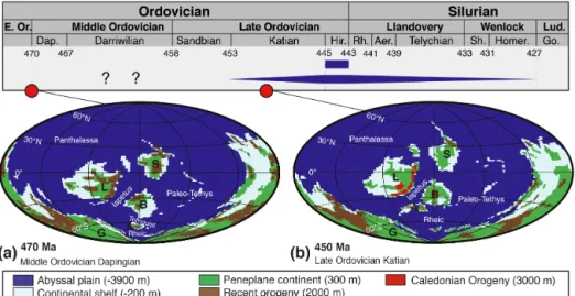
Figure 1. Continental configurations with the FOAM ocean grid based on the paleogeographical reconstructions from Blakey (2007), with the color code for the bathymetric and topographic categories used in this study. G: Gondwana, A: Avalonia, B: Baltica, L: Laurentia, S: Siberia. Ocean names are shown. Each time slice is replaced on the synthetic Ordovician glaciation chronology (inspired from Finnegan et al., 2011). Age limits are taken from the geological time scale v2014/02 (International Commission on Stratigraphy, 2014). Question marks are time intervals when hypothetical first ice sheets may have appeared according to Turner et al. (2012). Blue bars represent the two scenarios considered today for the duration of the Ordovician glaciation (see Sect. 2.2. for a full description).
2.2 Experimental setup
Spjeldnaes (1962), working on floro–faunal data, was the first to postulate a glaciation during the Ordovician. Since then, numerous studies widely documented the Ordovician glacial sedimentary record in North Africa (e.g., Beuf et al., 1971; Denis et al., 2007; Ghienne et al., 2007), South Africa (e.g., Young et al., 2004) and South America (e.g., Díaz-Martínez and Grahn, 2007). Dating these deposits remains highly difficult (e.g., Díaz-Martínez and Grahn, 2007) and geochemical methods bring conflicting results (see for ex-ample Trotter et al., 2008 and Finnegan et al., 2011). As a consequence, the duration of the glaciation is still not well constrained. Two models are still debated: a short-lived (< 2 Myr) glaciation limited to the Late Ordovician Hirnan-tian (445–443 Ma) (Brenchley et al., 1994, 2003; Sutcliffe et al., 2000), or a long-lived glaciation (> 20 Myr) that ex-tended from the Late Ordovician Katian to the Silurian Wen-lock, with the Hirnantian only representing the glacial maxi-mum (Saltzman and Young, 2005; Loi et al., 2010; Finnegan et al., 2011) (Fig. 1). Some authors even propose a Darriwil-ian ice age based on eustatic cyclicities (Turner et al., 2012). In this study, simulations were carried out for two paleo-geographical configurations reconstructed by Blakey (2007), one for 470 Ma (Middle Ordovician Dapingian) and one for 450 Ma (Late Ordovician Katian) (Fig. 1). These two re-constructions have been chosen to be respectively represen-tative of the following: (i) the pre-glacial interval; (ii) the undisputable Late Ordovician glacial interval. The 450 Ma reconstruction is considered here as a good estimate for the Late Ordovician Hirnantian (445 Ma). The
paleogeographi-cal changes are limited at that timespaleogeographi-cale and they are assumed to not critically impact global climate. Since previous studies have revealed the major role played by the topography to ini-tiate glacial conditions during the Ordovician (Crowley and Baum, 1995), we defined five realistic topographic classes (Fig. 1). The ocean model bathymetry is a flat-bottom case. As Ordovician vegetation was limited to non-vascular plants (Steemans et al., 2009; Rubinstein et al., 2010) – the cover-age of these can hardly be estimated – we imposed a bare soil (rocky desert) at every land grid point. No ice sheet was pre-scribed on the land. The solar luminosity was set 3.5 % below present according to the model of solar physics provided by Gough (1981), and we used the “cold summer orbital con-figuration” (CSO). The CSO is defined with an obliquity of 22.5◦, an eccentricity of 0.05 and a longitude of perihelion of 270◦. Because most explanatory hypotheses require a major
pCO2 fall to initiate glacial conditions in the Middle–Late Ordovician (Brenchley et al., 1994; Kump et al., 1999; Villas et al., 2002; Lenton et al., 2012), we finally used five pCO2 values representative for presumed Ordovician conditions: 4, 6, 8, 12 and 16 PAL. A lower value, 2 PAL, was also tested in order to better understand the climatic behavior although this
pCO2 clearly stands beyond the lower bound of the pCO2 range defined for the Ordovician Period. For each simula-tion, the model was run until deep ocean equilibrium was reached, which means 2000 years of integration except for the 450 Ma experiment with the pCO2set to 6 PAL that re-quired 1000 years more.
Atmospheric surface temperature (°C) pCO2 (PAL) 2X 4X 6X 8X 12X 16X pCO2 (PAL) 2X 4X 6X 8X 12X 16X 120 100 80 60 40 20 0 0 5 10 15 20 25 COOL mode WARM mode tipping-point
Mean annual global sea ice cover
(10 6 km 2) (a) (b) FOAM slab, 450 Ma FOAM slab, 470 Ma FOAM, 450 Ma FOAM, 470 Ma
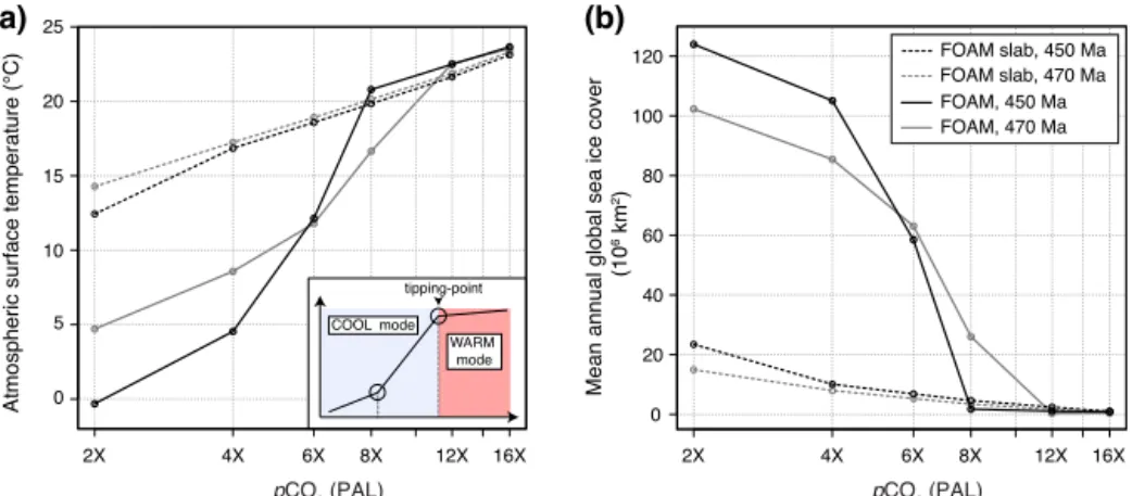
Figure 2. (a) Mean annual, globally averaged surface air temperature for various pCO2values from 2 to 16 PAL, with the slab-version of
FOAM and with the fully coupled ocean–atmosphere–sea ice version of FOAM at 470 and at 450 Ma. The sketch illustrates the explanations provided in the main text. Note the logarithmic scale on the x axis. (b) Same plot as (a), for the mean annual global sea ice cover expressed in M km−2.
Figure 3. SST (color shading) and permanent sea ice cover (blue-white shading) simulated at 450 Ma with the fully coupled version of FOAM within the cold climatic mode (at 6 PAL) and within the warm climatic mode (at 8 PAL). The permanent sea ice cover is de-fined as the sum of all grid points whose at least 80 % of the surface is covered by sea ice during a year, allowing to discard temporary sea ice cover by icebergs or rapidly advancing and retreating ice fronts. The gray mask stands for continental masses.
3 Climate simulation results
3.1 Sensitivity to an atmospheric CO2decrease
Figure 2 presents the relationship between the global mean surface air temperature (SAT) and the pCO2for all the simu-lations discussed in this paper. For comparison with the pre-vious studies undertaken with slab oceans (Crowley et al., 1993; Crowley and Baum, 1995; Gibbs et al., 1997; Her-rmann et al., 2003, 2004b), we first ran FOAM with a 50 m
deep mixed-layer slab ocean (black dashed lines in Fig. 2). All boundary conditions were kept the same as for the runs with the ocean–atmosphere GCM (see Sect. 2.2) and we fol-lowed the usual conventions by setting the diffusion coef-ficient so that total OHT reaches its present value. As ex-pected from previous studies, the Late Ordovician (450 Ma) climate system is sensitive to a pCO2 decrease and the temperature–CO2 relationship is linear in a log-axis graph (Fig. 2a). The model sensitivity, 3◦C per halving of CO2, lies very close to the value 2.5◦C obtained by Herrmann et al. (2003). It is however noteworthy that, for an identical atmospheric forcing value, climate is systematically warmer compared to GENESIS (Gibbs et al., 1997; Herrmann et al., 2004b). An immediate explanation lies in the prescribed so-lar constant. We chose a soso-lar constant 3.5 % weaker than today following the parametric law from Gough (1981). Pre-vious studies mostly used a 4.5 % depressed insolation com-pared to present-day (Crowley and Baum, 1995; Gibbs et al., 1997; Herrmann et al., 2003, 2004b), following the constant rate of decrease of 1 % every hundred million years proposed by Crowley and Baum (1992). Both values are within the range −3.5 to −5 % defined by Endal and Sofia (1981), but our weaker decrease of the solar constant logically results in higher temperatures. We must note that modeled absolute temperatures are also sensitive to ice albedo and cloud pa-rameterizations and are thus highly model-dependent (see for example Braconnot et al., 2012). Proposing absolute climate estimates for the Ordovician remains highly challenging and lies far beyond the main purpose of our study. Aside that ab-solute temperature offset, FOAM produces a trend similar to results previously published when it is used as a slab.
Using the same (450 Ma) paleogeographical configura-tion, FOAM experiments with ocean dynamics lead to a much different climatic response to the CO2forcing. The temperature-CO2 relationship is non-linear (Fig. 2a). Two
0 80°S 40°S 0° 40°N 80°N 20 -20 -40 -60 450Ma-16X 450Ma-12X 450Ma-8X 450Ma-6X 450Ma-4X 450Ma-2X Latitude
Surface air temperature (°C)
Figure 4. Mean annual, zonally averaged SAT simulated for each
pCO2at 450 Ma with the fully coupled version of FOAM.
climatic modes are simulated as forcing parameters slowly change.
– For high CO2 concentrations (≥ 8 PAL), the warm mode is marked by a hot climate (Figs. 2a and 3) and no sea ice in the Northern Hemisphere (NH) (Figs. 2b and 3). The model sensitivity is similar to the one ob-tained with the slab (3◦C per halving of CO2) and lies within the range 2.1–4.7◦C defined with various up-to-date GCMs for present-day simulations (IPCC, 2013). The temperature decrease associated to a CO2drop is almost evenly distributed at all latitudes (Fig. 4). – When atmospheric forcing is decreased from 8 to
4 PAL, the annual global mean SAT falls by 8.65◦C
from 8 to 6 PAL, and by 7.6◦C from 6 to 4 PAL. The
Ordovician climate abruptly enters a cool climatic mode characterized by a fast extension of the sea ice cover (Figs. 2, 3 and 5). A tipping point is reached, a slight
pCO2 drop leading to a sharp cooling. The tempera-ture decrease associated to a halving of CO2 (from 8 to 4 PAL), −16◦C, lies far beyond the IPCC (2013) upper bound. The SAT drop is unevenly distributed against the latitudes. The minimum mean annual cool-ing is observed in the tropics (up to −5◦C from 8 to 6 PAL) whereas the maximum cooling (up to −27◦C from 8 to 6 PAL) occurs in both hemispheres at polar latitudes (Fig. 4). The amplification of the thermal re-sponse at high latitudes is due to the sea ice albedo pos-itive feedback. The hemispheric sea ice cover (Table 1, Fig. 5b and c) suggests in particular a strong relation-ship between the NH sea ice extension and the global climate state. No ice is present in the NH within the warm mode (Fig. 3), and it is the expansion of the sea ice from the North Pole that marks the shift to the cold climatic mode. It is noteworthy here that the simulation of the sea ice in the model FOAM has been proven cor-rect enough in the modern climate to be reasonably ex-tended to paleoclimate studies. The reader is invited to
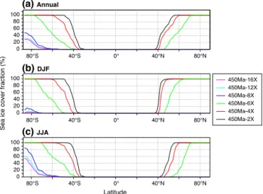
80°S 40°S 0° 40°N 80°N 0 20 40 60 80 100 0 20 40 60 80 100 0 20 40 60 80 100 80°S 40°S 0° 40°N 80°N 80°S 40°S 0° 40°N 80°N
Sea ice cover fraction (%)
Latitude (a) Annual (b) DJF (c) JJA 450Ma-16X 450Ma-12X 450Ma-8X 450Ma-6X 450Ma-4X 450Ma-2X
Figure 5. Zonally averaged sea ice cover fraction (expressed in percents) simulated for each pCO2at 450 Ma with the fully cou-pled version of FOAM. DJF: December, January and February. JJA: June, July and August.
refer to the study from Lefebvre et al. (2012, paragraph 14) for the whole analysis.
– From 4 to 2 PAL, the Earth’s climate is still in cold mode but the SAT drop tends to slow down. Another thresh-old is crossed and the model sensitivity decreases back to a level characteristic of glacial climate (∼ 5◦C per CO2halving, see Berner and Kothavala, 2001). The cli-mate change does not differ so much from the cooling occurring within the warm climatic mode between 16 and 8 PAL for a corresponding halving of CO2, though glacial conditions still provide a higher global sensitiv-ity (Kothavala et al., 1999) and an enhanced polar cool-ing. Sea ice continues to grow almost with the same in-tensity in the Southern Hemisphere (SH) but its spread is very limited in the NH (Table 1), where the sea ice edge stabilizes near 40◦N (Fig. 5a).
The simulations were replicated for the 470 Ma continen-tal configuration. A similar evolution is observed. With the slab model (Fig. 2), the temperature-CO2relationship is still linear in the log-axis graph. For the coupled runs (Fig. 2 and Table 1), two phases of stable climate are separated by a ma-jor climatic instability within the interval 12–6 PAL. The tip-ping point showing the shift from the warm to the cold cli-matic mode is reached this time between 12 and 8 PAL and is still associated to a sudden extension of the sea ice in the NH. Three main conclusions follow from theses results: (i) the climatic instability originates in ocean dynamics, as it is not observed with the slab, (ii) NH sea ice cover plays a crit-ical role in the shift to the cold climatic mode, (iii) reaching the cold climatic mode requires a lower CO2level at 450 Ma than at 470 Ma.
Table 1. Overview of the coupled simulations. The name of each experiment includes the age of the paleogeography used in input followed by the pCO2expressed in PAL. These abbreviations are used throughout the manuscript. Slab runs are not shown.
Surface Global Mean annual Mean annual Mean annual Simulations pCO2 air temperature global sea Southern Hemisphere Northern Hemisphere
(ppm) temperature of the Ocean ice cover sea ice cover sea ice cover (◦C) (◦C) (106km2) (106km2) (106km2) 450 Ma-2X 560 −0.3 1.8 123.9 49.3 74.6 450 Ma-4X 1120 4.5 2.5 105.1 35.2 69.9 450 Ma-6X 1680 12.1 4.1 58.5 15.5 43.0 450 Ma-8X 2240 20.8 9.0 1.8 1.8 0.0 450 Ma-12X 3360 22.5 11.4 1.1 1.1 0.0 450 Ma-16X 4480 23.7 12.7 0.9 0.9 0.0 470 Ma-2X 560 4.7 2.3 102.3 28.3 74.0 470 Ma-4X 1120 8.6 3.1 85.4 19.2 66.2 470 Ma-6X 1680 11.8 3.9 63.1 10.9 52.2 470 Ma-8X 2240 16.7 6.7 26.0 3,2 22.8 470 Ma-12X 3360 22.5 11.1 0.3 0.3 0.0 470 Ma-16X 4480 23.5 12.0 0.4 0.4 0.0
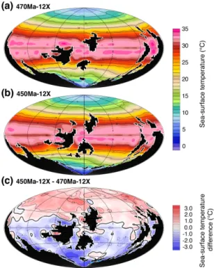
Figure 6. Comparison of the SST simulated at 12 PAL with the fully coupled version of FOAM for the two continental configurations used in this study. The black mask stands for continental masses. Note that, for the plot presented in (c), the mask actually represents all the grid points where the SST difference could not be calculated, cumulating each point that is a continent either in the 450 or in the 470 Ma configuration.
This type of non-linearity within the Earth climate system has been extensively studied in the past few years. We will in particular discuss our results in the light of the major studies from Rose and Marshall (2009) and Ferreira et al. (2011) in
Sect. 4, but we propose for now to continue our analysis by focusing on the response of ocean dynamics to the paleogeo-graphical changes occurring between 470 and 450 Ma. 3.2 Sensitivity of ocean dynamics to the paleogeography The shift from the warm to the cold climatic mode occurs between 12 and 8 PAL at 470 Ma, and between 8 and 6 PAL at 450 Ma. In order to constrain why the 450 Ma climatic system has a lower CO2threshold, we compare the climatic features at both time slices for the same pCO2. We use the simulations preceding the tipping points (12 PAL) to identify the preconditioning factors for the climatic instability. These two simulations have a same global SAT (22.5◦C, Table 1) and a close global ocean temperature (11.1◦C at 470 Ma and 11.4◦C at 450 Ma, Table 1) that make the comparison rea-sonable.
Figure 6 displays the sea-surface temperatures (SST) for the 470 Ma-12X and the 450 Ma-12X experiments together with the SST difference between these two simulations. From 470 to 450 Ma, the SH cools and the NH warms (Fig. 6c). The temperature changes are on the order of a few degrees, lo-cally up to 3◦C in both hemispheres. Assuming that the NH sea ice extension plays a major role in the abrupt transition from one climatic state to another through the sea ice albedo positive feedback (see Sect. 3.1), the NH warming observed in Fig. 6c appears as the key point accounting for the increas-ing stability from 470 to 450 Ma. It becomes more difficult to form sea ice and thus to trigger the albedo feedback in the NH through time, and a lower CO2concentration is required to enter the cool climatic mode at 450 Ma.
The origin of the temperature pattern observed in Fig. 6c is investigated through the study of the oceanic heat trans-port (Fig. 7). From 470 to 450 Ma, the NH is marked by
0.8 0.4 0.0 -0.4 -0.8 -1.2 -1.6 -2.0
(a) Total (b) Advective
1.0 0.0 -1.0 -2.0 1.6 1.2 0.8 0.4 0.0 -0.4 -0.8 (c) Diffusive -1.5 -0.5 0.5 1.5 Present-day 450Ma-12X 470Ma-12X
Oceanic heat transport (PW)
80°S 40°S 0° 40°N 80°N
Latitude 80°S 40°S Latitude0° 40°N 80°N 80°S 40°S Latitude0° 40°N 80°N
Figure 7. Comparison of the total, advective and diffusive OHT simulated with the fully coupled version of FOAM at 12 PAL for the two continental configurations used in this study. The OHT is given in petawatts (1 PW = 1015W). The present-day curve is the control experiment conducted at present-day conditions with the up-to-date IPSL (Institut Pierre Simon Laplace) CM4 GCM (see the main text for explanations).
Figure 8. Siberia’s northward drift and the consequences on the lon-gitudinal stream function. Eastward stream is positive (red), west-ward stream is negative (blue). The stream function is integrated over the whole water column. S: Siberia. Simulations were con-ducted with the fully coupled version of FOAM. It is noteworthy that the northward drift of Siberia from the Middle to the Late Or-dovician is a robust feature of all available OrOr-dovician paleogeo-graphical reconstructions published so far, including the maps from Torsvik and Cocks (Cocks and Torsvik, 2007, Fig. 6a; Torsvik and Cocks, 2013: Fig. 2.12, 2.14 and 2.15), Golonka and Gaweda (2012, Figs. 6 and 7) and Scotese and McKerrow (1991, Figs. 4 and 5).
a significant increase in the northward OHT exceeding 100 % at 20◦N (from 0.4 to 0.8 PW respectively, Fig. 7a). In the SH, a slight decrease in the southward OHT is observed at all lat-itudes except for a narrow latitudinal band between 6 and 18◦S (Fig. 7a). This new energy redistribution brings more heat to the NH and less to the SH. As a direct consequence, the NH warms from 470 to 450 Ma, and the SH cools.
Dividing the total OHT into its advective and diffusive components (Fig. 7b and c) reveals a striking feature within the NH advective heat transport between ∼ 35 and ∼ 65◦N (Fig. 7b). The transport is negative, meaning a southward heat transport, which is a priori unexpected in the NH. The advective heat transport scales as ∼ 9 × 1T × ρ ×
Cpwhere 9 is the strength of the overturning circulation, 1T the temperature difference between the northward and
the southward limbs of the overturning circulation, ρ the wa-ter density and Cp the water specific heat. A negative heat
transport implies a southward transport of surface warm wa-ters. The southward water flow results from an intense wind-driven eastward circumpolar current that develops at these latitudes in the absence of landmasses (Fig. 8). As a conse-quence of the Ekman deflection, the water masses are devi-ated to the right of the main eastward stream and thus con-stitute a southward mass transport. From 470 to 450 Ma, the northward drift of Siberia (Fig. 8) inhibits the zonal current and the associated Ekman cell, explaining why the reverse OHT weakens through time (Fig. 7b). A similar reverse ad-vective OHT is observed in present-day experiments in the SH due to the Antarctica Circumpolar Current. Figure 7b shows the results obtained for a present-day experiment con-ducted with a state-of-the-art ocean–atmosphere–vegetation coupled model: the IPSL CM4 GCM (Marti et al., 2010). A reverse heat transport is obtained near 40◦S. From this point of view, the Ordovician quasi-oceanic NH keeps some common features with our present-day ∼ 80 % oceanic SH.
The global Northern Hemisphere OHT strengthening, from 470 to 450 Ma (Fig. 7a), is due to an increase of the transport in three main areas (Fig. 9), the location of which turns out to be constrained by changes in the overturning cir-culation (Fig. 10).
– Between 5 and 30◦N, the advective OHT increases (Fig. 7b) in response to the intensifying surface subtrop-ical cell that directly brings heat from the equator. – Between 30 and ∼ 42◦N, the diffusive OHT increases
(Fig. 7c) as a consequence of the strengthening of the subtropical cell. Much more heat is “deposited” at 30◦N, which imposes a strong temperature gradient. Heat diffuses from the warm tropical latitudes where the heat is “deposited” to the cold waters at higher latitudes. – Between ∼ 42 and 60◦N, the southward advective OHT weakens through time (Fig. 7b). The northward drift of Siberia inhibits the 40◦N zonal current (Fig. 8): the
counter-clockwise cell associated to the zonal current acts over the entire water column at 470 Ma and not beyond 2500 m at 450 Ma. Hence less cold waters are brought from the high latitudes to the mid-latitudes re-sulting in an increased net northward heat transport. An additional process is the northward deflection of surface warm currents by Siberia at 450 Ma. This can be seen by comparing the isotherms 20 and 15◦C in Fig. 6a and b. Although it is restricted to upper levels oceanic wa-ters, this second mechanism is significant because the first tens of meters represent an important heat reservoir of the ocean.
The most significant outstanding issue is to determine why the temperature drawdown occurring through the tipping point is sharper at 450 than at 470 Ma. Although the tip-ping point occurs at lower CO2 at 450 Ma, the two paleo-geographical configurations present almost the same global SAT and an equivalent sea ice cover at 6 PAL (Fig. 2 and Table 1). Paradoxically, this sharper response through the 450 Ma tipping point is due to the paleogeographically in-duced increase in the Northern Hemisphere OHT that previ-ously inhibited the cooling. While the NH warms from 470 to 450 Ma (Fig. 6c), the NH equator-to-pole temperature profile flattens (not shown here). These changes are observed within the warm mode at 12 PAL, but they are critical since they constitute the preconditioning factors for the differential cli-matic sensitivity as climate shifts to the cold clicli-matic mode. The flattened 450 Ma SST gradient delays the tipping point to a certain extent by inhibiting sea ice growth at polar lat-itudes, but it increases the global climate sensitivity to the radiative forcing as soon as NH sea ice begins to expand.
4 Discussion
The potential existence of multiple equilibria in the climate system has a long story in the literature. Lorenz (1968) discussed whether the physical laws governing climate are “transitive”, supporting a unique climate state, or “intran-sitive” leading to several sets of long-term statistics. Two main mechanisms supporting climate intransitivity have so far emerged. The first mechanism originates in the study of Stommel (1961) who showed that the thermohaline circula-tion may sustain two stable regimes depending on whether the driver of the circulation, the density difference, is dom-inated by the temperature or the haline gradient, leading re-spectively to an intense or a weak circulation. This concept motivated later a wealth of studies linking the last glacial abrupt events to these multiple thermohaline states, studies that are today well known as “fresh water hosing” experi-ments (see for example Kageyama et al., 2013). The second mechanism is the ice albedo positive feedback. It was inde-pendently introduced by Budyko (1969) and Sellers (1969). The authors developed simple one-dimension climate mod-els in which surface temperature is computed by taking into
80°S 40°S 0° 40°N 80°N 1.20 0.80 0.40 0.00 -0.40 -0.80 OHT dif ference (PW) Latitude total advective diffusive 450Ma-12X - 470Ma-12X
Figure 9. Difference in total, advective and diffusive OHT between the 450 Ma-12X and the 470 Ma-12X simulations.
account the local radiative budget and the meridional heat transport. Two stable climate states are obtained for a same solar forcing depending on the initial conditions, describing a classical hysteresis loop: a warm state with a small sea ice cap or no sea ice at all (Eq3, Fig. 11a), and a cold completely ice-covered state (Eq1, Fig. 11a). A large sea ice cap of finite size extending to the mid-latitudes constitutes another analyt-ical solution, but this third equilibrium turns out to be very unstable and thus not realizable (Eq2 in Fig. 11a; Rose and Marshall, 2009). Critical non-linearities are observed at both latitudinal extremes (Rose and Marshall, 2009 and references therein). At low latitudes, near the equator, the “large ice cap instability” rules. An sea ice margin reaching these latitudes expands up to the equator (“snowball” state Eq1, Fig. 11a). At very high latitudes, this is the “small ice cap instability” (SICI): a reduced sea ice cover will either completely disap-pear or spread until it forms a small ice cap restricted to the high latitudes (warm state, Eq3 in Fig. 11a). In the absence of the equilibrium Eq2, a unique sea ice cap of large (beyond the SICI domain) but finite (no snowball state) size is obtained for a given climatic forcing (Fig. 11b). A comprehensive re-view of the successive improvements associated to the energy balance models (EBMs) is provided by North et al. (1981).
Recently, Rose and Marshall (2009) managed to stabi-lize the equilibrium Eq2 by extending the previous EBMs through two key processes: (i) the effect by which sea ice in-sulates the ocean surface from the atmosphere, (ii) the wind-driven structure of the OHT. A primary maximum at low-latitudes accounts for the heat transport by the subtropical gyre and a secondary maximum at high latitudes for the OHT generated by the subpolar gyre, with a local minimum in be-tween (Fig. 11c). Contrary to classical EBMs in which the OHT describes a large parabolic curve from the equator to the pole (Fig. 11b), the OHT pattern from Rose and Mar-shall (2009) shows a local minimum at mid-latitudes where the sea ice edge can stably rest. This OHT structure is closer to the observations (see for example Garnier et al., 2000). Within the improved EBM of Rose and Marshall (2009), the small ice cap instability does not exist anymore: sea ice
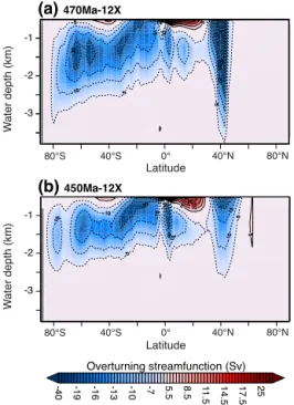
80°S 40°S 0° 40°N 80°N 80°S 40°S 0° 40°N 80°N -1 -2 -3 -1 -2 -3 W ater depth (km) Overturning streamfunction (Sv) Latitude Latitude -40 -19 -16 -13 -10 -7 5.5 8.5 11.5 14.5 17.5 25 W ater depth (km) (a) 470Ma-12X (b) 450Ma-12X
Figure 10. Comparison of the global meridional overturning circu-lation simulated at 12 PAL with the fully coupled version of FOAM for the two continental configurations used in this study. Red shad-ing and solid contours indicate a clockwise circulation, blue shadshad-ing and dashed contours indicate a counter-clockwise circulation.
caps of various size can persist at polar latitudes. Because the equilibrium Eq2 is now stable, two sea ice caps of large but finite size can be sustained for the same climatic forcing (e.g., for F5 in Fig. 11c). The position of the sea ice edge in the equilibrium Eq2 is captured within the position of the mid-latitude OHT minimum and thus very stable when ex-ternal forcing is varied.
The question however still remained if the mid-latitude equilibrium Eq2 would hold in a more complex climate model with many degrees of freedom and a strong internal variability. Ferreira et al. (2011) demonstrated multiple equi-libria using an up-to-date ocean GCM (the MITgcm) on two idealized configurations: a purely aqua planet, and an ocean planet with a strip of land extending from one pole to the other. The three states from Rose and Marshall (2009) are obtained: (i) a warm, ice-free state, (ii) a cold state with sea ice extending down to mid-latitudes, (iii) and the completely ice-covered “snowball” state. The authors highlight the con-sistency of their results with the study of Rose and Mar-shall (2009). In their complex GCM, the multiple equilibria owe their existence to the latitudinal structure of the OHT. The authors moreover extend the previous results from Rose and Marshall (2009) by demonstrating that no OHT mini-mum is required. A weak high-latitude OHT within the sub-polar gyre is sufficient to stabilize a finite sea ice cap at mid-latitudes, in that critical weak-OHT zone situated between
the subtropical and the subpolar gyres that they widely refer to as the “OHT convergence”.
Here, we have investigated the Ordovician climate sensi-tivity to a varying radiative forcing. The hallmark of our re-sults is the existence of a global climatic instability in the NH. A tipping point separates two climatic modes: a warm mode with no sea ice in the NH, and a cold mode with sea ice extending down to the mid-latitudes (Fig. 5a). In the light of the results from Rose and Marshall (2009) and Ferreira et al. (2011), these climatic modes respectively correspond to the classical warm mode obtained with an EBM and to the third equilibrium previously described, respectively Eq3 and Eq2 in Fig. 11. The simulations marked by a weak pCO2 sta-bilize in Eq2, whereas the experiments conducted with high CO2levels lead to the warm state of Eq3.
It is noteworthy that the latitudinal position at which the sea ice edge stabilizes within the cold climatic mode ef-fectively lies immediately poleward of the Northern Hemi-sphere OHT convergence (Fig. 12, ∼ 40◦N), which is a key prediction from Rose and Marshall (2009) and Ferreira et al. (2011). According to these authors, the strong low-latitude OHT encounters here a weaker transport and heat is “deposited”, thus preventing the sea ice edge from moving further equatorward.
The fact that the ice edge is strongly enslaved to the OHT convergence (Fig. 12; Rose and Marshall, 2009) ex-plains why the model returns to its initial sensitivity below 4 PAL (see Sect. 3.1). Ice cannot spread further and stabi-lizes. The sea ice albedo feedback is geometrically stopped by the subtropical high-OHT barrier and cooling is conse-quently slowed-down.
The comparison of Fig. 11b and c permits to explain why tipping points were not previously observed for the Ordovi-cian. Similarly to the classical EBMs, the slab models use a purely diffusive transport. The resulting OHT describes the same large parabolic curve from the equator to the pole (Fig. 12). There is no OHT minimum or more largely no OHT convergence where the sea ice edge could rest to make the mid-latitude equilibrium stable. Climate cannot switch between stable states which inhibits the climatic instability.
In addition, the similarity between EBMs and slab models explains the results from Gibbs et al. (1997) who observed with the slab model GENESIS a runaway icehouse that they interpreted as resulting from the small ice cap instability. As it was previously explained, this mechanism is not observed anymore when the OHT structure is taken into account, but it is a classical feature of the EBMs and by extension of all models that use a diffusive OHT. We emphasize that the run-away icehouse proposed by Gibbs et al. (1997) and the cli-matic instability suggested in this study rely on much differ-ent mechanisms.
The absence of ocean dynamics in the slab models makes their response to an atmospheric forcing much different from the ocean–atmosphere GCM when simulating time periods of particular land-sea configuration as it is the case for the
Eq 30° 60° 90° LICI SICI 30° 60° 90° 30° 60° 90°
(a)
(b)
(c)
Sea ice front latitude
Forcing (W
.m
-2)
Forcing (W
.m
-2)
Forcing (W
.m
-2)
F1 F2 F3 F4OHT
(PW)
OHT
(PW)
F5Eq1 Eq2 Eq3
Eq2 Eq3 Eq3
+
+
-+
-0
+
0
Figure 11. (a) Graph showing the latitude of the sea ice front (x axis) vs. the climatic forcing (y axis) for a classical Budyko–Sellers type EBM. Dark arrows indicate the pathway de-scribed by the model through a whole cycle of forcing decrease and increase. Red arrows account for major climatic instabilities. Red circles represent the sea ice edge latitudes corresponding to each analytical solution for a given climatic forcing F1. Dashed lines represent regions that are correct analytical solutions, but are un-able to be realized within the model due to instability. SICI: small ice cap instability; LICI: large ice cap instability. (b) represents the same plot as (a), while focusing on the domain shaded in grey in (a). The forcing is decreased and then increased without reaching the snowball equilibrium Eq1. Several forcing values (F2, F3 and F4) are represented, each one leading to a single sea ice cap of fi-nite size (red circles). The OHT pattern corresponding to the purely diffusive transport characteristic of classical EBMs is overlayed in grey (right y axis). (c) Same plot as (b) for the extended EBM from Rose and Marshall (2009) (see the main text for explanations) in which the OHT pattern is modified (grey curve). Note the two sea ice caps of finite size corresponding to the forcing level F5. (a) is adapted from North et al. (1981), (b) and (c) are modified after Rose and Marshall (2009). 80°S 40°S 0° 40°N 80°N 1.0 0.0 -1.0 -2.0 Latitude
Oceanic heat transport (PW)
450Ma-6X 450Ma-4X 450Ma-2X
Sea ice extent (DJF) 450 Ma OHT at 8 PAL
FOAM slab FOAM
Figure 12. Comparison of the total OHT at 450 Ma and at 8 PAL for the slab version of FOAM and for the fully coupled version of FOAM. The OHT pattern is relatively stable when CO2is varied. Color bars represent the maximum (boreal winter) Northern Hemi-sphere sea ice extent simulated within the cold climatic mode at 450 Ma with the fully coupled model.
Ordovician. An efficient way to overcome that apparent de-ficiency would be to impose the structure of the latitudi-nal OHT, as Rose and Marshall (2009) did in their ex-tended EBM. The decisive answer is brought by Ferreira et al. (2011), who tested this hypothesis within the MIT-gcm used as a slab. With the simple diffusive coefficient, the mid-latitude equilibrium is not stable, as for classical EBMs. However, by imposing the OHT deduced from their coupled runs to the slab, they managed to reproduce exactly the same climatic response as with their complex GCM. These results confirm that the differential behavior of ocean–atmosphere and slab–atmosphere GCMs lies within ocean dynamics through the OHT.
The Ordovician Period turned out to bring a favorable paleogeographical context to propose the sudden shift be-tween different climate states on a realistic configuration. The stabilization of a sea ice edge at mid-latitudes requires a wind-driven latitudinal OHT structure, a condition that can be reached only in an oceanic context. It is notably the case of the Ordovician 95 % oceanic NH which ocean zonal cir-culation is not hampered by continental masses. If conti-nents were largely distributed at all latitudes, then continental edges would strongly alter the pattern originally imposed by the winds and by the Ekman pumping mechanism. The OHT may thus be more even at all latitudes, as it is the case in our study in the SH due to the supercontinent Gondwana (Figs. 1 and 12). No OHT convergence would be obtained and the OHT pattern would become very similar to the one imposed by a simple diffusion coefficient. From this point of view, it is logical that the global instability lies in our study in the oceanic NH, and it would anyway be inconceivable to obtain a similar behavior in the SH.
5 Conclusions
We have examined the response of the Ordovician climate to a decreasing pCO2for two continental configurations at 470 and at 450 Ma with the coupled ocean, atmosphere and sea ice GCM FOAM. We have found the existence of tipping points in the Ordovician climate owing to the particular pale-ogeography with a quasi-oceanic Northern Hemisphere. As a result, the climate may have abruptly shifted from a warm climatic mode to a cold climatic mode. Warm SST and no sea ice in the NH characterize the warm mode, whereas much colder SST and a large sea ice extension to the mid-latitudes mark the cool mode. We also note that subtle changes occur-ring in the continental configuration between 470 and 450 Ma make the latter less sensitive to the radiative forcing. Indeed, the shift from the warm to the cold climatic mode takes place between 12 and 8 PAL at 470 Ma, and between 8 and 6 PAL at 450 Ma. One potential mechanism relies on the changes occurring in the oceanic heat transport between the two sim-ulated time periods. The paleogeographical evolution pro-motes a larger northward oceanic heat transport at 450 Ma which in turn induces warmer Northern Hemisphere SST. Spread of sea ice becomes more difficult and a lower CO2 level is required to enter the cold climatic mode. The fact that the tipping point is reached for a higher CO2 level at 470 Ma whereas climate was warm at that time (e.g., Trotter et al., 2008), implies that the pCO2must have been high dur-ing the Middle Ordovician, thus precluddur-ing climate to reach the climatic instability.
The tipping point is due to a climatic instability occurring in the quasi-oceanic Northern Hemisphere. The instability relies on the sudden shift from a warm climate to a climatic equilibrium characterized by a sea ice front resting at mid-latitudes. This particular climate state has been widely dis-cussed in the literature and proven to require a wind-driven latitudinal structure of the OHT (Rose and Marshall, 2009; Ferreira et al., 2011). The classical EBMs and slab models use a purely diffusive OHT and are by construction unable to stabilize an ice edge at the mid-latitudes (Rose and Mar-shall, 2009; Ferreira et al., 2011), explaining why that be-havior was never noticed in previous studies about the Or-dovician climate (e.g., Gibbs et al., 1997; Herrmann et al., 2004b). Published studies performed with idealized land–sea configurations however demonstrate that this limitation may be overcome by imposing a latitudinally varied diffusion coefficient reproducing the OHT structure. Such extended EBMs and slab models successfully reproduce the behavior of the more complex ocean–atmosphere GCMs (Rose and Marshall, 2009; Ferreira et al., 2011).
The Late Ordovician Hirnantian is characterized by the rapid growth of large ice sheets (e.g., Ghienne et al., 2007; Loi et al., 2010; Finnegan et al., 2011). Recent geochemi-cal data suggest an abrupt tropigeochemi-cal SST cooling at that time (Trotter et al., 2008; Finnegan et al., 2011). Several CO2 sinks have been proposed to explain cooling but no
consen-sus has been found so far (Brenchley et al., 1994; Kump et al., 1999; Villas et al., 2002; Lenton et al., 2012). In this context, the tipping point becomes a very interesting working hypoth-esis. It requires only a slight CO2 decrease and at the same time induces a sharp global temperature drawdown, in the same order of magnitude as the Hirnantian cooling observed by Trotter et al. (2008) and Finnegan et al. (2011). The cli-matic instability demonstrated in this study therefore repre-sents a step forward in understanding the Ordovician glacial events and provides in particular a minimal hypothesis for the Hirnantian abrupt cooling and associated glacial pulse. Our results also shed a new light on the CO2sinks envisaged to reduce the pCO2at that time. We now suggest that a mod-erate sink (e.g., Young et al., 2009; Nardin et al., 2011) may have been sufficient, thus making relevant some mechanisms that have been neglected so far because of their moderate im-pact on the pCO2.
Acknowledgements. We thank Mark Williams and one anonymous
referee for their constructive remarks that have greatly improved this paper. We thank Pierre Sepulchre for providing the IPSL CM4 GCM run. We are also grateful to David G. Ferreira for his constructive and helpful comments. This work was granted access to the HPC resources of TGCC under the allocation 2014-012212 made by GENCI.
Edited by: A. Haywood
References
Berner, R. A.: GEOCARBSULF: a combined model for Phanero-zoic atmospheric O2and CO2, Geochim. Cosmochim. Ac., 70,
5653–5664, doi:10.1016/j.gca.2005.11.032, 2006.
Berner, R. A. and Kothavala, Z.: GEOCARB III: a revised model of atmospheric CO2 over Phanerozoic time, Am. J. Sci., 301,
182–204, doi:10.2475/ajs.301.2.182, 2001.
Beuf, S., Biju-Duval, B., De Charpal, O., Rognon, P., Gariel, O., and Bennacef, A.: Les grès du Paléozoïque Inférieur au Sahara, Technip, Paris, 464 pp., 1971.
Blakey, R. C.: Carboniferous-Permian paleogeography of the as-sembly of Pangea, in: Fifteenth International Congress on Car-boniferous and Permian Stratigraphy, edited by: Wong, T. E., Utrecht, the Netherlands, pages 443–465, Royal Netherlands Academy of Arts and Sciences, Amsterdam, 2007.
Braconnot, P., Harrison, S. P., Kageyama, M., Bartlein, P. J., Masson-Delmotte, V., Abe-Ouchi, A., Otto-Bliesner, B., and Zhao, Y.: Evaluation of climate models using palaeoclimatic data, Nat. Clim. Change, 2, 417–424, doi:10.1038/NCLIMATE1456, 2012.
Brenchley, P. J., Marshall, J. D., Carden, G., Robertson, D., Long, D., Meidla, T., Hints, L., and Anderson, T. F.: Bathy-metric and isotopic evidence for a short-lived Late Ordovician glaciation in a greenhouse period, Geology, 22, 295–298, doi:10.1130/0091-7613(1994)022<0295:BAIEFA>2.3.CO;2, 1994.
Brenchley, P. J., Carden, G. A., Hints, L., Kaljo, D., Mar-shall, J. D., Martma, T., Meidla, T., and Nõlvak, J.:
High-resolution stable isotope stratigraphy of Upper Ordovician se-quences: constraints on the timing of bioevents and environ-mental changes associated with mass extinction and glacia-tion, Geol. Soc. Am. Bull., 115, 89–104, doi:10.1130/0016-7606(2003)115<0089:HRSISO>2.0.CO;2, 2003.
Budyko, M. I.: The effect of solar radiation variations on the climate of the Earth, Tellus, 21, 611–619, doi:10.1111/j.2153-3490.1969.tb00466.x, 1969.
Cocks, L. R. M. and Torsvik, T. H.: Siberia, the wandering north-ern terrane, and its changing geography through the Palaeozoic, Earth-Sci. Rev., 82, 29–74, doi:10.1016/j.earscirev.2007.02.001, 2007.
Crowley, T. J. and Baum, S. K.: Toward reconciliation of Late Ordovician (∼ 440 Ma) glaciation with very high CO2 levels, J. Geophys. Res.-Atmos., 96, 22597–22610,
doi:10.1029/91JD02449, 1991.
Crowley, T. J. and Baum, S. K.: Modeling late Paleo-zoic glaciation, Geology, 2, 507–510, doi:10.1130/0091-7613(1992)020<0507:MLPG>2.3.CO;2, 1992.
Crowley, T. J. and Baum, S. K.: Reconciling Late Ordovician (440 Ma) glaciation with very high (14X) CO2levels, J.
Geo-phys. Res.-Atmos., 100, 1093–1101, doi:10.1029/94JD02521, 1995.
Crowley, T. J., Baum, S. K., and Kim, K. Y.: General cir-culation model sensitivity experiments with pole-centered supercontinents, J. Geophys. Res.-Atmos., 98, 8793–8800, doi:10.1029/93JD00122, 1993.
Denis, M., Buoncristiani, J.-F., Konate, M., Ghienne, J.-F., and Guiraud, M.: Hirnantian glacial and deglacial record in SW Djado Basin (NE Niger), Geodin. Acta, 20, 177–195, doi:10.3166/ga.20.177-195, 2007.
Dera, G. and Donnadieu, Y.: Modeling evidences for global warm-ing, Arctic seawater freshenwarm-ing, and sluggish oceanic circulation during the Early Toarcian anoxic event, Paleoceanography, 27, PA2211, doi:10.1029/2012PA002283, 2012.
Díaz-Martínez, E. and Grahn, Y.: Early Silurian glaciation along the western margin of Gondwana (Peru, Bolivia and northern Argentina): Palaeogeographic and geodynamic setting, Palaeo-geogr. Palaeocl., 245, 62–81, doi:10.1016/j.palaeo.2006.02.018, 2007.
Donnadieu, Y., Goddéris, Y., and Bouttes, N.: Exploring the cli-matic impact of the continental vegetation on the Mezosoic atmospheric CO2 and climate history, Clim. Past, 5, 85–96,
doi:10.5194/cp-5-85-2009, 2009.
Endal, A. S. and Sofia, S.: Rotation in solar-type stars, I – Evolu-tionary models for the spin-down of the sun, Astrophys. J., 243, 625–640, doi:10.1086/158628, 1981.
Ferreira, D., Marshall, J., and Rose, B.: Climate determinism revis-ited: multiple equilibria in a complex climate model, J. Climate, 24, 992–1012, doi:10.1175/2010JCLI3580.1, 2011.
Finnegan, S., Bergmann, K., Eiler, J. M., Jones, D. S., Fike, D. A., Eisenman, I., Hughes, N. C., Tripati, A. K., and Fischer, W. W.: The magnitude and duration of Late Ordovician-Early Silurian glaciation, Science, 331, 903–906, doi:10.1126/science.1200803, 2011.
Garnier, E., Barnier, B., Siefridt, L., and Béranger, K.: Investi-gating the 15 years air-sea flux climatology from the ECMWF re-analysis project as a surface boundary condition for ocean
models, Int. J. Climatol., 20, 1653–1673, doi:10.1002/1097-0088(20001130)20:14<1653::AID-JOC575>3.0.CO;2-G, 2000. Ghienne, J.-F., Le Heron, D., Moreau, J., Denis, M., and
Dey-noux, M.: The Late Ordovician glacial sedimentary system of the North Gondwana platform, in: Glacial sedimentary processes and products, Special Publication, edited by: Hambrey, M., Christoffersen, P., Glasser, N., Janssen, P., Hubbard, B., and Siegert, M., 39, 295–319, International Association of Sedimen-tologists, Blackwells, Oxford, 2007.
Gibbs, M. T., Barron, E. J., and Kump, L. R.: An at-mospheric pCO2 threshold for glaciation in the Late
Ordovician, Geology, 25, 447–450, doi:10.1130/0091-7613(1997)025<0447:AAPCTF>2.3.CO;2, 1997.
Golonka, J. and Gaweda, A.: Plate tectonic evolution of the south-ern margin of Laurussia in the Paleozoic, in: Tectonics – Recent advances, edited by: Sharkov, E., 261–282, InTech, 2012. Gough, D. O.: Solar interior structure and luminosity variations,
Sol. Phys., 74, 21–34, doi:10.1007/BF00151270, 1981. Herrmann, A. D., Patzkowsky, M. E., and Pollard, D.:
Obliquity forcing with 8–12 times preindustrial lev-els of atmospheric pCO2 during the Late Ordovician
glaciation, Geology, 31, 485–488, doi:10.1130/0091-7613(2003)031<0485:OFWTPL>2.0.CO;2, 2003.
Herrmann, A. D., Haupt, B. J., Patzkowsky, M. E., Seidov, D., and Slingerland, R. L.: Response of Late Ordovician pa-leoceanography to changes in sea level, continental drift, and atmospheric pCO2: potential causes for long-term
cool-ing and glaciation, Palaeogeogr. Palaeocl., 210, 385–401, doi:10.1016/j.palaeo.2004.02.034, 2004a.
Herrmann, A. D., Patzkowsky, M. E., and Pollard, D.: The impact of paleogeography, pCO2, poleward ocean heat
transport and sea level change on global cooling during the Late Ordovician, Palaeogeogr. Palaeocl., 206, 59–74, doi:10.1016/j.palaeo.2003.12.019, 2004b.
International Commission on Stratigraphy: International Chronos-tratigraphic Chart v2014/02, available at: www.stratigraphy.org, 2014.
IPCC: Climate Change 2013: The physical science basis, in: Con-tribution of Working Group I to the Fifth Assessment Report of the Intergovernmental Panel on Climate Change, edited by: Stocker, T. F., Qin, D., Plattner, G.-K., Tignor, M., Allen, S. K., Boschung, J., Nauels, A., Xia, Y., Bex, V., and Midgley, P. M., Cambridge University Press, Cambridge, UK and New York, NY, USA, 1535 pp., 2013.
Jacob, R. L.: Low frequency variability in a simulated atmosphere ocean system, Ph.D. thesis, University of Wisconsin-Madison, 1997.
Kageyama, M., Merkel, U., Otto-Bliesner, B., Prange, M., Abe-Ouchi, A., Lohmann, G., Ohgaito, R., Roche, D. M., Sin-garayer, J., Swingedouw, D., and Zhang, X.: Climatic impacts of fresh water hosing under Last Glacial Maximum conditions: a multi-model study, Clim. Past, 9, 935–953, doi:10.5194/cp-9-935-2013, 2013.
Kiehl, J. T., Hack, J. J., Bonan, G. B., Boville, B. A., Williamson, D. L., and Rasch, P. J.: The national cen-ter for Atmospheric Research community climate model: CCM3, J. Climate, 11, 1131–1149, doi:10.1175/1520-0442(1998)011<1131:TNCFAR>2.0.CO;2, 1998.
Kothavala, Z., Oglesby, R. J., and Saltzman, B.: Sensitivity of equilibrium surface temperature of CCM3 to systematic changes in atmospheric CO2, Geophys. Res. Lett., 26, 209–212, doi:10.1029/1998GL900275, 1999.
Kump, L. R., Arthur, M. A., Patzkowsky, M. E., Gibbs, M. T., Pinkus, D. S., and Sheehan, P. M.: A weathering hypothesis for glaciation at high atmospheric pCO2 during the Late
Ordovi-cian, Palaeogeogr. Palaeocl., 152, 173–187, doi:10.1016/S0031-0182(99)00046-2, 1999.
Lefebvre, V., Donnadieu, Y., Sepulchre, P., Swingedouw, D., and Zhang, Z.-S.: Deciphering the role of southern gateways and car-bon dioxide on the onset of the Antarctic Circumpolar Current, Paleoceanography, 27, PA4201, doi:10.1029/2012PA002345, 2012.
Lenton, T. M., Crouch, M., Johnson, M., Pires, N., and Dolan, L.: First plants cooled the Ordovician, Nat. Geosci., 5, 86–89, doi:10.1038/ngeo1390, 2012.
Loi, A., Ghienne, J.-F., Dabard, M. P., Paris, F., Botquelen, A., Christ, N., Elaouad-Debbaj, Z., Gorini, A., Vidal, M., Videt, B., and Destombes, J.: The Late Ordovician glacio-eustatic record from a high-latitude storm-dominated shelf succession: the Bou Ingarf section (Anti-Atlas, Southern Morocco), Palaeogeogr. Palaeocl., 296, 332–358, doi:10.1016/j.palaeo.2010.01.018, 2010.
Lorenz, E. N.: Climatic determinism, Meteor. Mon., 8, 1–3, 1968. Marti, O., Braconnot, P., Dufresne, J. L., Bellier, J., Benshila, R.,
Bony, S., Brockmann, P., Cadule, P., Caubel, A., Codron, F., No-blet, N., Denvil, S., Fairhead, L., Fichefet, T., Foujols, M. A., Friedlingstein, P., Goosse, H., Grandpeix, J. Y., Guilyardi, E., Hourdin, F., Idelkadi, A., Kageyama, M., Krinner, G., Lévy, C., Madec, G., Mignot, J., Musat, I., Swingedouw, D., and Ta-landier, C.: Key features of the IPSL ocean atmosphere model and its sensitivity to atmospheric resolution, Clim. Dynam., 34, 1–26, doi:10.1007/s00382-009-0640-6, 2010.
Nardin, E., Goddéris, Y., Donnadieu, Y., Le Hir, G., Blakey, R. C., Pucéat, E., and Aretz, M.: Modeling the early Paleozoic long-term climatic trend, Geol. Soc. Am. Bull., 123, 1181–1192, doi:10.1130/B30364.1, 2011.
North, G. R., Cahalan, R. F., and Coakley, J. A.: Energy bal-ance climate models, Rev. Geophys., 19, 91–121, 80R1502, doi:10.1029/RG019i001p00091, 1981.
Pancost, R. D., Freeman, K. H., Herrmann, A. D., Patzkowsky, M. E., Ainsaar, L., and Martma, T.: Recon-structing Late Ordovician carbon cycle variations, Geochim. Cosmochim. Ac., 105, 433–454, doi:10.1016/j.gca.2012.11.033, 2013.
Pollard, D.: A retrospective look at coupled ice sheet – climate mod-eling, Climate Change, 100, 173–194, doi:10.1007/s10584-010-9830-9, 2010.
Poulsen, C. J. and Jacob, R. L.: Factors that inhibit snow-ball Earth simulation, Paleoceanography, 19, PA4021, doi:10.1029/2004PA001056, 2004.
Poussart, P. F., Weaver, A. J., and Barnes, C. R.: Late Or-dovician glaciation under high atmospheric CO2: a
cou-pled model analysis, Paleoceanography, 14, 542–558, doi:10.1029/1999PA900021, 1999.
Rose, B. E. J. and Marshall, J.: Ocean heat transport, sea ice, and multiple climate states: insights from energy balance models, J. Atmos. Sci., 66, 2828–2843, doi:10.1175/2009JAS3039.1, 2009.
Rubinstein, C. V., Gerrienne, P., de la Puente, G. S., Astini, R. A., and Steemans, P.: Early Middle Ordovician evidence for land plants in Argentina (eastern Gondwana), New Phytol., 188, 365–369, doi:10.1111/j.1469-8137.2010.03433.x, 2010. Saltzman, M. R. and Young, S. A.: Long-lived glaciation
in the Late Ordovician? Isotopic and sequence-stratigraphic evidence from western Laurentia, Geology, 33, 109–112, doi:10.1130/G21219.1, 2005.
Scotese, C. R. and McKerrow, W. S.: Ordovician plate tectonic re-constructions, in: Advances in Ordovician geology, edited by: Barnes, C. R. and Williams, S. H., 90–9, 271–282, Geological Survey of Canada, 1991.
Sellers, W. D.: A global climatic model based on the energy balance of the earth-atmosphere system, J. Appl. Meteorol., 8, 392–400, doi:10.1175/1520-0450(1969)008<0392:AGCMBO>2.0.CO;2, 1969.
Semtner Jr, A. J.: A model for the thermodynamic growth of sea ice in numerical investigations of cli-mate, J. Phys. Oceanogr., 6, 379–389, doi:10.1175/1520-0485(1976)006<0379:AMFTTG>2.0.CO;2, 1976.
Servais, T., Owen, A. W., Harper, D. A., Kröger, B., and Munnecke, A.: The Great Ordovician Biodiversification Event (GOBE): the palaeoecological dimension, Palaeogeogr. Palaeocl., 294, 99–119, doi:10.1016/j.palaeo.2010.05.031, 2010. Sheehan, P. M.: The late Ordovician mass extinction, Annu. Rev. Earth Pl. Sc., 29, 331–364, doi:10.1146/annurev.earth.29.1.331, 2001.
Spjeldnaes, N.: Ordovician climatic zones, Norsk Geol. Tidsskr., 41, 45–77, 1962.
Steemans, P., Le Herissé, A., Melvin, J., Miller, M. A., Paris, F., Verniers, J., and Wellman, C. H.: Origin and radiation of the earliest vascular land plants, Science, 324, 353–353, doi:10.1126/science.1169659, 2009.
Stommel, H.: Thermohaline convection with two stable regimes of flow, Tellus, 13, 224–230, doi:10.1111/j.2153-3490.1961.tb00079.x, 1961.
Sutcliffe, O. E., Dowdeswell, J. A., Whittington, R. J., Theron, J. N., and Craig, J.: Calibrating the Late Ordovi-cian glaciation and mass extinction by the eccentricity cy-cles of Earth’s orbit, Geology, 28, 967–970, doi:10.1130/0091-7613(2000)28<967:CTLOGA>2.0.CO;2, 2000.
Torsvik, T. H. and Cocks, L. R. M.: New global palaeogeographical reconstructions for the Early Palaeozoic and their generation, in: Early Palaeozoic biogeography and palaeogeography, edited by: Harper, D. A. T. and Servais, T., 38, 5–24, Geological Society of London, Memoirs, 2013.
Trotter, J. A., Williams, I. S., Barnes, C. R., Lécuyer, C., and Nicoll, R. S.: Did cooling oceans trigger Ordovician biodiver-sification? Evidence from conodont thermometry, Science, 321, 550–554, doi:10.1126/science.1155814, 2008.
Turner, B. R., Armstrong, H. A., Wilson, C. R., and Makhlouf, I. M.: High frequency eustatic sea-level changes during the Middle to early Late Ordovician of southern Jordan: Indirect evidence for a Darriwilian Ice Age in Gondwana, Sediment. Geol., 251, 34–48, doi:10.1016/j.sedgeo.2012.01.002, 2012.
Vandenbroucke, T. R., Armstrong, H. A., Williams, M., Paris, F., Zalasiewicz, J. A., Sabbe, K., Nõlvak, J., Challands, T. J., Verniers, J., and Servais, T.: Polar front shift and atmo-spheric CO2 during the glacial maximum of the Early
Pa-leozoic Icehouse. P. Natl. Acad. Sci., 107, 14983–14986, doi:10.1073/pnas.1003220107, 2010.
Villas, E., Vennin, E., Álvaro, J. J., Hammann, W., Herrera, Z. A., and Piovano, E. L.: The late Ordovician carbonate sedimentation as a major triggering factor of the Hirnantian glaciation, B. Soc. Geol. Fr., 173, 569–578, doi:10.2113/173.6.569, 2002.
Yapp, C. J. and Poths, H.: Ancient atmospheric CO2
pres-sures inferred from natural goethites, Nature, 355, 342–344, doi:10.1038/355342a0, 1992.
Young, G. M., Minter, W., and Theron, J. N.: Geochemistry and palaeogeography of upper Ordovician glaciogenic sedimentary rocks in the Table Mountain Group, South Africa, Palaeogeogr. Palaeocl., 214, 323–345, doi:10.1016/j.palaeo.2004.07.029, 2004.
Young, S. A., Saltzman, M. R., Foland, K. A., Linder, J. S., and Kump, L. R.: A major drop in seawater87Sr/86Sr during the Mid-dle Ordovician (Darriwilian): Links to volcanism and climate?, Geol., 37, 951–954, doi:10.1130/G30152A.1, 2009.
Zhang, Z.-S., Yan, Q., and Wang, H.-J.: Has the Drake passage played an essential role in the Cenozoic cooling?, Atmos. Ocean. Sci. Lett., 3, 288–292, 2010.