HAL Id: hal-02305269
https://hal.inria.fr/hal-02305269
Preprint submitted on 4 Oct 2019
HAL is a multi-disciplinary open access
archive for the deposit and dissemination of
sci-entific research documents, whether they are
pub-lished or not. The documents may come from
teaching and research institutions in France or
abroad, or from public or private research centers.
L’archive ouverte pluridisciplinaire HAL, est
destinée au dépôt et à la diffusion de documents
scientifiques de niveau recherche, publiés ou non,
émanant des établissements d’enseignement et de
recherche français ou étrangers, des laboratoires
publics ou privés.
Multi-Scale Approximation of Thin-Layer Flows on
Curved Topographies
Yih-Chin Tai, Jeaniffer Vides, Boniface Nkonga, Chih-Yu Kuo
To cite this version:
Yih-Chin Tai, Jeaniffer Vides, Boniface Nkonga, Chih-Yu Kuo. Multi-Scale Approximation of
Thin-Layer Flows on Curved Topographies. 2019. �hal-02305269�
Multi-Scale Approximation of Thin-Layer Flows on Curved
Topographies
Yih-Chin Tai⇤
Department of Hydraulic and Ocean Engineering, National Cheng Kung University, Tainan, Taiwan Jeani↵er Vides
LEMMA R&D Service, Sophia Antipolis, Biot, France & Maison de la Simulation, Gif-sur-Yvette, France Boniface Nkonga
Universit´e Cˆote d’Azur (UCA), LJAD Nice & Inria Sophia Antipolis - M´editerran´ee, France Chih-Yu Kuo
Research Center for Applied Sciences, Academia Sinica, Taipei, Taiwan
Abstract
This paper is devoted to a multi-scale approach for describing the dynamic behaviors of thin-layer flows on complex topographies. Because the topographic surfaces are generally curved, we introduce an appropriate coordinate system for describing the flow behaviors in an efficient way. In the present study, the complex surfaces are supposed to be composed of a finite number of triangle elements. Due to the unequal orientation of the triangular elements, the distinct flux directions add to the complexity of solving the Riemann problems at the boundaries of the triangular elements. Hence, a vertex-centered cell system is introduced for computing the evolution of the physical quantities, where the cell boundaries lie within the triangles and the conventional Riemann solvers can be applied. Consequently, there are two mesh scales: the element scale for the local topographic mapping and the vertex-centered cell scale for the evolution of the physical quantities. The final scheme is completed by employing the HLL-approach for computing the numerical flux at the interfaces. Three numerical examples (the Ritter’s solution, the Stoker’s solution and the parabolic similarity solution) and one application to a large-scale landslide are conducted to examine the performance of the proposed approach as well as to illustrate its capability in describing the shallow
⇤Corresponding author
Email address: yctai@mail.ncku.edu.tw (Yih-Chin Tai)
Manuscript
flows on complex topographies.
Keywords: multi-scale approach, complex topography, shallow flows, unstructured mesh, vertex-centered formulation
1. Introduction
Most geophysical hazardous flows take place over complex topographies. Consider, for example, the occurrence of avalanches, landslides or debris flows over non-trivial topographies in mountainous areas. Not surprisingly, there is a strong link between the particular flow path and the geometry of the underlying basal topography. In addition, these flows are generally “thin” in comparison
5
with its extension in its tangential direction, so that the term “shallow flow” is employed here to characterize thin flows on curved surfaces. For this type of flows, it is customary to make use of the incompressibility with shallowness assumption to asymptotically derive reduced models for the evolution of the depth averaged velocity and the thickness of the flow. Conventionally, these models are given in Cartesian coordinates and reduced through depth-integration process, where
10
the topography is added on the horizontal plane. As the depth-averaged models generally employ the shallowness assumption, in which the computed velocities are parallel to the corresponding coordinate axes instead of the exact basal surface, a high variation in topography leads to significant deviation in representing the depth-averaged velocity. To overcome this shortcoming, [1] first applied a 2D curvilinear coordinate system aligned with the curved bed for modeling granular flows. This
15
2D curvilinear coordinate system is extended to 3D by introducing a simple reference surface curved in the down-slope direction, and the complex topography is described by superposing a shallow basal topography on it [2, 3, 4, 5]. Although the concept of simple curved reference plane has been widely adopted, it su↵ers from the limitation of the predefined unique down-slope direction of the simple curved reference surface, especially in its application to snaking canyon terrain. Pudasaini and
20
Hutter [6] improved it by imposing a curved and twisted coordinate system, in which the thalweg coincides with the projection of the master curve on the reference surface. However, it is not free from the challenge of thalweg splitting/merging in a complex canyon terrain.
Bouchut and Westdickenberg [7] proposed shallow water equations in a general coordinate sys-tem, which does not only fix the drawback of the above constrains (either the unique down-slope
di-25
rection or single thalweg) but also points out the way in modeling shallow flows over non-trivial topo-graphic surfaces. Following [7] and integrating its concept with the unified coordinate method [8, 9],
a non-conventional approach is proposed for geophysical mass flows. The non-conventional approach simplifies the complicate computation caused by the Christo↵el symbols in the model equations [10] and allows the topography variation caused by erosion or deposition [11, 12]. With this
non-30
conventional description, an application to real event of large scale is illustrated in [13]. Recently, the single-phase model employed in [13] has been extended to the two-phase approach [14], in which the phase separation and sediment-concentrated snout can be well reproduced. Taking into account the non-hydrostatic (excess) pore-water pressure for the fluid constituent [15, 16] and hypoplastic intergranular stress, Heß et al. [17] amended two additional fields and proposed the model equations
35
in the general coordinate system.
The above mentioned models are mainly hyperbolic and finite volume methods are often used for their numerical approximation. In general, the approximation strategies are structured as follows:
• Construction of a global coordinate system, relying on the assumption that the surface de-scription can be defined analytically;
40
• Representation of the conservative laws, relative to the global coordinate system; • Reduction of the model equations with shallowness assumption and scaling analysis; • Representation of the surface with a finite number of elements;
• Approximation of the reduced model using the discrete surface.
In the context of engineering applications, it is presumptuous to expect that an analytical
formu-45
lation of the ground surface is attainable. However, from data provided by geographic information systems (GIS), one can casually extract a discrete description of the surfaces that drive thin flows. As a result, it is more practical to use this discrete description as the starting point of the resolution strategy, and this is the kind of approach that will be adopted in this work. Subsequently, we will locally define two mesh scales: the element scale and the cell scale. The discrete mapping and the
50
reduced model are both defined at the element scale, and the average values that evolve in time are defined at the cell scale [18, 19].
In section 2, we present the model, which is divided into 6 subsections, from the “local element scale parameterization” to the “final scheme for weakly sheared shallow flows”. Next, the developed strategy is validated in Section 3 and applied to a real event by back-calculating the plausible flow
55
2. Discrete Sub-Scale Model and Reduction
Let us start by considering a surface 2 R3 that represents the basal topographic surface.
Formally, we have = 8 < :exxx = 0 @ xxx b 1 A 2 R3, where xxx = 0 @ x y 1 A 2 ⌦ ⇢ R2 and b = b(xxx) 9 = ;,
being z = b(xxx) the equation defining the basal surface. Unfortunately, this analytical description is not always available and, in general, we must settle for approximated surfaces that are piecewise defined: h= [ e Ee' , whereEe⌘ ⇣ e xxxi,xxexj, xxexk ⌘
are non-overlapping flat triangular surfaces defined by the points
e x x xi= 0 @ xxxi b (xxxi) 1 A , exxxj= 0 @ xxxj b (xxxj) 1 A and xxxek= 0 @ xxxk b (xxxk) 1 A . y x Ee e x xxk e xxxj e x xxi e x x xj e x x xk e x x xi
C
e iC
i Ee y x(a) Triangular surface element: Ee (b) Dual cell construction
Figure 1: ElementEe, cellCiand the sub-cellCei associated to the cellCiand the elementEe.
This strategy for the representation of the basal surface is similar to the one used in [20], but therein the numerical strategy considers the control volumes to be the triangles (cell-centered
approach). Instead, in this work we make use of dual cells in a vertex-centered formulation. For each elementEe, three sub-cells can be obtained by connecting the centroid of the element’s face
with the midpoints of the edges, as depicted in Figure 1a. Thus, by using the element scale, the cell scale is obtained from the union of the sub-cells associated to the mesh vertex and its neighboring elements (see Figure 1b). Each control cellCiis then defined as
Ci=
[
e2E(i)
Ce i
Although the cellCiis made of planar surfaces, it is generally non-planar so that we can estimate
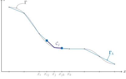
an approximate curvature to be used for numerical purposes; an example of non-planar dual cells in the one-dimensional case is shown in Figure 2. Also note that the elementEecan be written as
60
the union of sub-cells such thatEe=Cie[ Cje[ Cke.
z
x
Cj
xi xij xj xjk xk
h
Figure 2: One-dimensional representation of non-planar dual cells.
2.1. Local Element Scale Parametrization
On each triangular surface, we introduce a local system of coordinates e⇠⇠⇠⌘ e⇠⇠⇠e; in what follows, we use e⇠⇠⇠ instead of e⇠⇠⇠e to simplify our writing. In addition, we introduce the following notation:
e⇠⇠⇠ = 0 @ ⇠⇠⇠ ⇣ 1 A , exxx = 0 @ xxx b(xxx) 1 A , exxx = 0 @ xxx z 1 A , eyyy = 0 @ xxx 0 1 A , (1a)
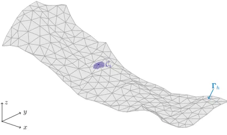
y x z
Ci
h
Figure 3: Two-dimensional representation of non-planar dual cells.
all specified in terms of the coordinate pairs
x x x = 0 @ x y 1 A and ⇠⇠⇠ = 0 @ ⇠ ⌘ 1 A . (1b)
In (1a), we have purposely introducedxxex once more to point out the di↵erence between it andxexx, i.e., the latter refers to the Cartesian coordinates in the three-dimensional space and the former to a point on the topographic surface. The basal surface on an elementE is defined as
b (xxx) = bi+ (bj bi) ⇤j(xxx) + (bk bi) ⇤k(xxx),
being ⇤m(xxx) (linear) barycentric coordinate functions on the Cartesian coordinates. For instance,
⇤i(xxx) = 1 ⇤j(xxx) ⇤k(xxx) with
⇤j(xxx) =
[(eyyy(xxx) eyyyi)⇥ (eyyyk eyyyi)]· beeez
[(eyyyj eyyyi)⇥ (eyyyk eyyyi)]· beeez , ⇤k(x
xx) =[(eyyy(xxx) eyyyi)⇥ (eyyyj eyyyi)]· beeez [(eyyyk eyyyi)⇥ (eyyyj eyyyi)]· beeez ,
where (beeex,beeey,beeez) is the standard Cartesian basis (inR3) andeyyy the Cartesian coordinates projected
on the plane z = 0, as defined in (1).
Now, the local basis associated to an element is defined by the vectors ggg⇠, ggg⌘and ggg⇣, where
ggg⇠=xexxj xexxi, ggg⌘=exxxk exxxi and ggg⇣ =
ggg⇠⇥ ggg⌘
and the local transformation on an element is e x
xx⇣e⇠⇠⇠⌘= ⇠ ggg⇠+ ⌘ ggg⌘+ ⇣ ggg⇣. (2)
The term ⇣ can be regarded as the distance above the basal surface; on the basal surface itself, ⇣ = ⇣e= 0. The vectors ggg⇠, ggg⌘and ggg⇣ are the covariant ones associated to the transformation. As
these local vectors are constant, we have
ggg⇠= @⇠xexx, ggg⌘= @⌘xxex and ggg⇣= @⇣xxex,
and the Jacobian of the transformation j = det @
@e⇠⇠⇠xexx !
= (ggg⇠⇥ ggg⌘)· ggg⇣. (3)
This transformation is compatible with the ones proposed in [7, 21], with the simplification that the current transformation is locally linear. As a consequence, the Jacobian and transformation matrices are constant. Indeed, simple calculations show that
@ @e⇠⇠⇠exxx = (ggg⇠, ggg⌘, ggg⇣) = 0 B B B @ @⇠x @⌘x c@xb @⇠y @⌘y c@yb @⇠b @⌘b c 1 C C C A= 0 B @ @⇠⇠⇠xxx sss 1 cssst@⇠⇠⇠xxx c 1 C A ,
with c = 1/p1 +k@xxxbk2, sss = c@xxxb and 1cssst@⇠⇠⇠xxx = (@⇠b, @⌘b). The rows of the inverse matrix @ @exxxe⇠⇠⇠ ⌘ ⇣ @ @e⇠⇠⇠xxxe ⌘ 1
are the contravariant vectors ggg⇠, ggg⌘and ggg⇣, specifically
✓ @ @exxxe⇠⇠⇠ ◆t = ggg⇠, ggg⌘, ggg⇣ = 0 B @ (iiiiiiiii sss⌦ sss) (@xxx⇠⇠⇠)t sss cssst(@ x x x⇠⇠⇠)t c 1 C A ,
where they follow the relations gggn· gggp= npwith npbeing the Kronecker delta.
65
We now have the choice to use hereafter either the matrices and sub-matrices of the transfor-mation (as in [7]) or the covariant and contravariant vectors (as was partially the case in [12]). For simplicity of the formulation, we subsequently employ the covariant and contravariant vectors and assume that the basal surface does not change with time. Then, for any vector uuu, the divergence rxexx· uuu in the Cartesian coordinates takes the following form with curvilinear coordinates:
jrexxx· uu = @u ⇠ juuu· ggg⇠ + @⌘(juuu· ggg⌘) + @⇣ juuu· ggg⇣ =re⇠⇠⇠·
⇣ j⇣@xexxe⇠⇠⇠
⌘ uuu⌘.
Moreover, for any symmetric tensor field PPP and a linear transformation (see, for instance, [7, Lemma 3.1, page 28]), we have
jrexxx· PPP = @⇠ jPPPggg⇠ + @⌘(jPPPggg⌘) + @⇣ jPPPggg⇣ =re⇠⇠⇠· (jPPPkkk) ,
with kkk =⇣@exxxe⇠⇠⇠
⌘t
. Thus, the divergence theorem in curvilinear coordinates reads Z ⌦re⇠⇠⇠· ⇣ j⇣@exxxe⇠⇠⇠ ⌘ u u u⌘ de⇠⇠⇠ = Z @⌦ ⇣ j⇣@exxxe⇠⇠⇠ ⌘ u u u⌘· n d eSe⇠⇠⇠= Z @⌦ juuu· ennn d eSe⇠⇠⇠, (4)
for the vector uuu, and Z
⌦re⇠⇠⇠· (jP P Pkkk) de⇠⇠⇠ = Z @⌦ jPPPnnn d ee Se⇠⇠⇠, (5)
for the tensor PPP, where the relationnnn d ee Se⇠⇠⇠⌘ kkk n d eSe⇠⇠⇠is carefully detailed in Appendix A.1.
2.2. Local Numerical Model
In order to use the most suitable reduced model for each element, it is desirable to also formulate the velocity field in the covariant and contravariant vectors, i.e.,
uuu = uxbeeex+ uybeeey+ uzbeeez= u⇠ggg⇠+ u⌘ggg⌘+ u⇣ggg⇣= u⇠ggg⇠+ u⌘ggg⌘+ u⇣ggg⇣,
for which one can notice that u⇠= uuu· ggg⇠, u⌘= uuu· ggg⌘and u⇣ = uuu· ggg⇣. In the local frame, the mass
and momentum conservative equations for an incompressible fluid read 8 > > < > > : @ @⇠ ju ⇠ + @ @⌘(ju ⌘) + @ @⇣ ju ⇣ = 0 , @ @t(juuu) + @ @⇠ h j uuuu⇠+ PPPggg⇠ i+ @ @⌘ h j (uuuu⌘+ PPPggg⌘)i+ @ @⇣ h j uuuu⇣+ PPPggg⇣ i= 0 , (6) where PPP =1 ⇢ ⇥ (p + ⇢g (z z0) )iiiiiiiii ⌧⌧⌧ ⇤
is a symmetric tensor representing the generalized stress tensor containing the gravity and ⇢ is the fluid density. These equations are in conservative form and are therefore suitable for finite volume approximations.
70
The considered flow is a free surface flow and we assume that the on the sub-cellCe
i, it has a
height he(t, ⇠⇠⇠) in the direction ggg⇣. The integration of system (6) over the local volumeVe i(t, e⇠⇠⇠) = [ ⇠⇠⇠ Ce i(⇠⇠⇠)⇥ [0, he(t, ⇠⇠⇠)] yields Z @Ve i juuu· ennn d = 0 , (7) @ @t Z Ve i juuu d⇠⇠⇠d⇣ ! Z Ce i juuu@thed⇠⇠⇠ + Z @Ve i j uuuuuu· ennn + PPPennn d = 0 , (8)
being @Ve
i the boundary of the volumeVie. This boundary can be decomposed into four entities
associated to the basal surface, to the free surface, to interactions with the other two neighboring cells, and to the boundary @e of the element e. This translates to
@Ve i = ⇣S ⇠⇠⇠Cei(⇠⇠⇠)⇥ {0} ⌘ S ⇣S ⇠⇠⇠Cie(⇠⇠⇠)⇥ {he(t, ⇠⇠⇠)} ⌘ [ j2#(i,e) 0 @[ ⇠⇠⇠ @Cie\ @Cje⇥ [0, he(t, ⇠⇠⇠)] 1 A[ 0 @[ ⇠⇠⇠ @Cie\ @e ⇥ [0, he(t, ⇠⇠⇠)] 1 A ,
where # (i, e) is the sub-set of cells neighbors to the cell i and associated to the element e. Let us now turn our attention to the surface integrals over this boundary.
75
Integrals associated to the basal surface: ⇣ = 0.
The normal vector at the basal surface is simply defined asnennd = ggg⇣d⇠⇠⇠. Then, the integrals over
Ce i (⇠⇠⇠)⇥ {0} become Z Ce i(⇠⇠⇠)⇥{0} juuu· ennn d = Z Ce i ju⇣ ⇣=0d⇠⇠⇠ , (9) Z Ce i(⇠⇠⇠)⇥{0} j (uuuuuu· ennn + PPPennn) d = Z Ce i j uuuu⇣+ PPPggg⇣ ⇣=0d⇠⇠⇠ . (10)
Integrals associated to the free surface: ⇣ = he(t, ⇠⇠⇠).
The normal vector at the free surface is such thatnennd = nd⇠⇠⇠, with n = ggg⇣ @
⇠heggg⇠ @⌘heggg⌘(we
refer the reader to Appendix A.1 for more details regarding n). The kinematic boundary condition at the free surface can be written as
@the= n· uuu. Then, we arrive at Z Ce i(⇠⇠⇠)⇥{he} juuu· ennn d = Z Ce i j@thed⇠⇠⇠ = @ @t Z Ce i jhed⇠⇠⇠ ! , (11) and Z Ce i(⇠⇠⇠)⇥{he} j (uuuuuu· ennn + PPPnnn) d =e Z Ce i juuu@thed⇠⇠⇠ + Z Ce i jPPPhnd⇠⇠⇠. (12) Note that the contribution of the integral following the equal sign in equation (12) will cancel out the contribution associated to the second term of equation (8).
Integrals associated to the interactions with the neighbor cells.
Let us recall that # (i, e) is the sub-set of cells neighbors to the cell i and associated to the element e. Then, for any j2 # (i, e), we compute the following fluxes:
h,e ij = Z @Ce i\@Cej Z he 0 juuu· ennn d⇣de` , (13) huuu,e ij = Z @Ce i\@Cej Z he 0 j (uuu⌦ uuu + PPP)nnen d⇣de` , (14)
wherenenn is the outward normal vector (see Figure 1b), later formulated in the covariant basis (refer to Appendix A.1).
85
After having obtained proper expressions for the surface integrals, we are now able to continue deriving the discrete model. On this account, let us first introduce the sub-scale variables hei and u u uei(t), defined by hei = 1 ae i Z Ce i jhed⇠⇠⇠ and he iuuuei(t) = 1 ae i Z Ve i juuude⇠⇠⇠, with ae i = Z Ce i jd⇠⇠⇠ .
Then, according to the previously established integrals (9)-(14), the evolution of hei and h e iuuuei,
contained in equations (7) and (8), can be reformulated as
@t ⇣ aeih e i ⌘ + X j2#(i,e) h,e ij = Z Ce i ju⇣ ⇣=0d⇠⇠⇠ Z @Ce i\@e Z he 0 juuu· ennn d⇣de` , (15) @t ⇣ ae ih e iuuu e i ⌘ + X j2#(i,e) huuu,e ij = Z Ce i j uuuu⇣+ PPPggg⇣ ⇣=0d⇠⇠⇠ Z Ce i j (PPPn)⇣=hd⇠⇠⇠ Z @Ce i\@e Z he 0 j (uuu⌦ uuu + PPP)nnn d⇣dee ` . (16)
Note that these sub-scale equations contain locally averaged and fluctuating quantities. More-over, we want to define the numerical scheme for quantities at the scale of the cell. For this, we wish to recall that each cellCihas been defined as the union of non-overlapping cellsCei, as shown
in Figure 1b. Consequently, the average onCican be obtained by summing equation (15) over the
words, for all e2 E (i), equations (15) and (16) are added to obtain, at the cell scale, 8 > > > > > > > > > > > > > > > > > > > < > > > > > > > > > > > > > > > > > > > : ai@thi + X e2E(i) X j2#(i,e) h,e ij = X e2E(i) Z Ce i ju⇣ ⇣=0d⇠⇠⇠ X e2E(i) Z @Ce i\@e Z he 0 juuu· ennn d⇣de` , ai@t hiuuui + X e2E(i) X j2#(i,e) huuu,e ij = X e2E(i) Z Ce i j uuuu⇣+ PPPggg⇣ ⇣=0d⇠⇠⇠ X e2E(i) Z Ce i j (PPPn)⇣=hd⇠⇠⇠ X e2E(i) Z @Ce i\@e Z he 0 j (uuu⌦ uuu + PPP)nnen d⇣de` , (17)
where we have defined aihi= X e2E(i) aeihei and aihiuuui= X e2E(i) aeiheiuuuei, being ai= X e2#(i)
aei the total area of the cellCi. It is noticed that the internal flux exchanges vanish
at the cell scale (cf. Figure 1), i.e., X e2E(i) Z @Ce i\@e Z he 0 juuu· ennn d⇣de` = 0 and X e2E(i) Z @Ce i\@e Z he 0 j (uuu⌦ uuu + PPP)nnn d⇣dee ` = 0 . (18)
Therefore, the cell scale discrete system (17) can be written in compact form
ai @ @twi+ X e2E(i) X j2#(i,e) Z @Ce i\@Cje Z he 0 jefff(w)nnen d⇣de` + X e2E(i) 0 @Z Ce i 0 @ 0 j PPPn 1 A d⇠⇠⇠ 1 A ⇣=h = X e2E(i) Z Ce i jefff(w) ggg⇣d⇠⇠⇠ ! ⇣=0 , (19) with w = 0 @ h huuu 1 A , w = 0 @ h huuu 1 A , and efff(w) = 0 @ uuut u u u⌦ uuu + PPP 1 A .
In the previous definitions, w = w + w0 is a local state composed of an average state w and its fluctuation w0.
The discrete model (19) has been obtained under certain assumptions (for instance, sub-cells are assumed to be flat). However, some of these assumptions can be relaxed without drastically changing the existing general formulation (19). At this moment, it is important to note that all the
components of the velocity are unknown to the discrete model. The evolution of wiwill be defined
as soon as the fluxes w,ei and the source terms Siw,e, terms on the right-hand side (RHS) of (19), are formulated as functions of the wj. A scheme with a reduced stencil is obtained when the flux
is a function of the neighboring cells’ averaged values.
Our aim is to now find a way to formulate the fluxes w,ei and source terms Sw,ei as functions of
95
the averaged values wj. For a common interface between two adjacent cells, this can be achieved
by the use of Riemann problems associated to an adapted reduced model. Other fluxes will be defined by means of the boundary conditions, particularly on the basal and free surfaces.
2.3. Shallowness Assumption
& Approximation Associated to Interactions with the Flow Surface
100
The shallowness approximations can be applied when the typical flow thickness is much smaller than the characteristic wavelength. In this context, the asymptotic analysis helps to justify that pressure is essentially due to the e↵ect of hydrostatic forces [12]. One can then use an approximation constructed so that the pressure at the flow surface is identically zero, namely
p' ⇢gc (⇣ h (t, ⇠⇠⇠) ) with c = ggg⇣· beee
z. This relation indicates the assumption that the curvature e↵ect is negligible, and
it is consistent with the fact that the basal surface is locally a flat triangle. However, as we can associate an approximated curvature at each vertex of the triangle, we can also add curvature e↵ect as in the reference [22], so that
p/⇢' (b+ gc) ⇣ h (t, ⇠⇠⇠) with b= ccc : (bbbuuu⌦ bbbuuu) ,
where ccc is an approximated curvature tensor and bbb = ggg⇠⌦ ggg
⇠+ ggg⌘⌦ ggg⌘ is the projection on the
tangent plane to the basal surface. On the other hand, with the considered mapping, we locally have
z z0= b (xxx) + c⇣ with b (xx) = b (xx xx (⇠⇠⇠) ) = bi z0+z (⇠⇠⇠) ,e
whereez (⇠⇠⇠) = ⇠ ggg⇠· beeez+ ⌘ ggg⌘· beeez. Then the generalized stress tensor PPP is approximated by
P P P =⇣p/⇢ + g (z z0) ⌘ iiiiiiiii ⌧⌧⌧ /⇢'⇣g (ch + b) b(⇣ h) ⌘ iiiiiiiii ⌧⌧⌧ /⇢ . (20) At the flow surface (⇣ = h), the stress tensor can be simplified as follows:
Then, the component of the stress flux associated to the free surface isotropic pressure ⇢g (ch + b) is reformulated to introduce a divergence form. Indeed,
g (ch + b) ggg⇠@ ⇠h + ggg⌘@⌘h = ggg⇠@⇠ ✓ gch 2 2 + gbh ◆ + ggg⌘@ ⌘ ✓ gch 2 2 + gbh ◆ ghrxxexb ,
where straightforward algebra givesrexxxb = ggg⇠@⇠ez + ggg⌘@⌘ez. Therefore, as n = ggg⇠@⇠h ggg⌘@⌘h + ggg⇣,
we get (PPPn)⇣=h= ggg⇠@ ⇠ ✓ gch 2 2 + gbh ◆ ggg⌘@ ⌘ ✓ gch 2 2 + gbh ◆ + ghrxexxb + g (ch + b) ggg⇣ ⇣=h 1 ⇢ ⌧⌧⌧ n ⇣=h.
Locally on a element, j, c, ggg⇠ and ggg⌘are constant; thus, we can perform an integration by parts in
order to obtain Z Ce i 0 @ 0 jPPPn 1 A ⇣=h d⇠⇠⇠ = X j2#(i,e) Z @Ce i\@Cej 0 B @ 0 j ✓ gch 2 2 + gbh ◆ iiiiiiiii 1 C A ennn de` Z @Ce i\@e 0 B @ 0 j ✓ gch 2 2 + gbh ◆ iiiiiiiii 1 C A ennn de` + Z Ce i 0 @ 0 jghrxxexb 1 A ⇣=h d⇠⇠⇠ + Z Ce i 0 @ 0 jg (ch + b) ggg⇣ 1 A ⇣=h d⇠⇠⇠ Z Ce i 0 @ 0 1 ⇢j ⌧⌧⌧ n 1 A ⇣=h d⇠⇠⇠ . (22)
Here, we have used the fact that the normal vector is constant on the interface @Ve
i \ @Vje that
contains @Ce
i \ @Cje. By using this decomposition, we artificially separate the contribution of the
free flow surface into several components. Usually, the first integral on the right-hand side of (22) is approximated as a lateral flow in the hyperbolic framework. The third to the last integrals of the same RHS will be considered as source terms. In fact, the coherence of all of these di↵erent approximations is one of the goals of the well-balanced schemes [23]. The contribution of the second integral, associated to interactions in the cell itself, will be canceled out at the cell level according to conservation considerations. Therefore, this contribution can be safely ignored at this scale. Note that the total flux associated to the interface @Ce
i \ @Cje is now w,e ij = Z @Ce i\@Cej Z h 0 jefff(w)nnen d⇣de` Z @Ce i\@Cej 0 B @ 0 j ✓ gch 2 2 + gbh ◆ iiiiiiiii 1 C A ennn de` .
Since we have PPP ' g (ch + b)iiiiiiiii ⌧⌧⌧ /⇢ b(⇣ h)iiiiiiiii, the first integral in the equation above is, approximately, Z @Ce i\@Cej Z h 0 jefff(w)ennn d⇣de`' Z @Ce i\@Cej j hefff(w)nenn de` ' Z @Ce i\@Cej j 0 @ huuu t huuu⌦ uuu +⇣gch2+ gbh + bh 2 2 ⌘ iiiiiiiii 1 A ennn de` Z @Ce i\@Cje 0 @ 0 1 ⇢j h ⌧⌧⌧nenn 1 A de`.
According to the previous simplifications, the flux w,eij is then decomposed into a hyperbolic component fff,eij and a viscosity component ⌧⌧⌧ ,eij , specifically
w,e ij ' f f f,e ij ⌧ ⌧ ⌧ ,e ij , (23) where fff,e ij = Z @Ce i\@Cje e(jnnen, w) de` and ⌧⌧⌧ ,e ij = Z @Ce i\@Cje j 0 @ 0 1 ⇢⌧⌧⌧nnen 1 A d⇣de`.
The normal flux e(jennn, w) at the interface is given by
e(jennn, w) = 0 @ jhuuu· ennn jhuuu (uuu· ennn) + j (gc + b) h2 2nnne 1 A = (jennn · ggg⇠) fff (w) + (jennn· ggg⌘) ggg (w) ,
being w = (h, huuu)t, fff⌘ fff (w) and ggg⌘ ggg (w), with
fff = 0 @ hu ⇠ huuuu⇠+ (gc + b) h2 2ggg ⇠ 1 A and ggg = 0 @ hu ⌘ huuuu⌘+ (gc + b) h2 2ggg ⌘ 1 A . (24)
2.4. Riemann Problem at the Interface Scale We proceed to describe how the numerical flux e
ijis computed as a function of the intermediate
state we
ij, solution of an appropriate Riemann problem. The flux e(nnn, w) is a linear function of
n n
n. Assuming that the approximated state we
ij does not vary along the interface, we have f ff,e ij = e neij, weij , with neij= Z @Ce i\@Cje jennn de` .
Refer to Appendix A.2 for the definitions of the cell interface normal vectors ne
ijon a flat triangular
element. Now, in order to obtain an approximation of the above flux, let us consider the following Riemann problem at the interface scale:
@ @tw + @ @n e(nnn, w) = 0 with w (t = 0, n) = 8 < : wl, if n < 0 wr, if n > 0 , (25)
where n is the coordinate associated to the direction nnn. This system is hyperbolic and the eigenvalues (assuming bconstant) are = uuu·nnn, = uuu·nnn
p
(gc + b) h and = uuu·nnn +
p
(gc + b) h . Then,
an approximate Riemann solver will define the flux at n = 0 as a function of the states wland wr,
e.g.,
ee(nnn, wl, wr) = 1
2[ (nnn, wl) + (nnn, wr) +|A| (wl wr)] , being A ' @
@w (nnn, w) an approximated Jacobian. For this form, one of the simplest approxi-mations is the so-called Rusanov solver that considers |A| = ⇣max
w | (w) |
⌘
iiiiiiiii. For an HLL-type scheme, the numerical flux takes the following simplified form instead:
ee(nnn, wl, wr) = Sr (n
nn, wl) Sl (nnn, wr) SlSr(wl wr)
Sr Sl
,
where Sland Sr are the maximum wave speeds traveling to the left and right, respectively. For the
first order approximation, the numerical flux is estimated as
fff,e ij ' e
e
ne
ij, wi, wj .
This approximation of the flux is conservative, i.e., the outward normal vector associated to the cellCjat the interface withCiwill be opposite to nije. In other words, neji= neij, and by simple
algebraic manipulations, one can show that ee ne
ji, wj, wi = e e
ne
ij, wi, wj .
Let us mention that the current flux is obtained under the strong assumption that, locally at the interface, the fluctuating state w is constant in the thin layer and acts like the mean value w. In order to improve the approximation of the interface flux, interpolations are often employed, via the MUSCL approach. The MUSCL reconstruction is a purely geometrical interpolation. It is also possible to proceed with certain physical interpolations that take into account the thin profile of the local flow, that is,
f f f,e ij ' 1 hij Z hij 0 ee ne ij, wi(⇠⇠⇠ij, ⇣) , wj(⇠⇠⇠ij, ⇣) d⇣ ,
where wi(⇠⇠⇠ij, ⇣) = wi+ w0i(⇠⇠⇠ij, ⇣) and wj(⇠⇠⇠ij, ⇣) = wj+ w0j(⇠⇠⇠ij, ⇣). The interface profiles defined
105
by w0
iand w0jmust be built under physical considerations. This profiling is inevitable for strongly
sheared flows. In [24, 25, 26], it is proposed to introduce new variables based on the evolution of the kinetic energy, in order to simplify this construction.
We find it convenient to review what we have so far: ai @ @twi+ X e2E(i) X j2#(i,e) fff,e ij = X e2E(i) X j2#(i,e) ⌧⌧⌧ ,e ij + X e2E(i) Z Ce i jefff(w) ggg⇣d⇠⇠⇠ ! ⇣=0 + X e2E(i) Z Ce i 0 @ 0 j⌧⌧⌧ n/⇢ jg (ch + b) ggg⇣ jghr e x x xb 1 A ⇣=h d⇠⇠⇠ . (26)
At this stage of the numerical scheme construction, we still need to derive approximations for the fluxes and pressure forces on the basal surface, as well as the e↵ect of the topography change, the
110
viscosity fluxes.
2.5. Approximation Associated to Interactions with the Basal Surface
We assume here that the basal surface is impermeable so that the velocity component normal to the bottom is zero, i.e.,
u⇣b ⌘ 0 .
For ease of description, the drag forces equilibrium at the basal surface is assumed to be P P Pbggg⇣ = gbggg⇣+1 ⇢ pb ggg ⇣· ⌧⌧⌧ bggg⇣ ggg⇣ 1 ⇢µ˜pb u uu kuuuk, (27) where the last term represents the Coulomb friction law (see, for instance, [27, 3]), with µ the friction coefficient and ˜pb = pb ggg⇣· ⌧⌧⌧bggg⇣ + the positive part of the normal stress on the basal
surface. The friction coefficient µ can be interpreted as the ratio between shear and normal stresses;
115
µ' k⌧⌧⌧k/|p|, see e.g., [28, 29].
In the context of long-wave laminar flows, the shear stress normal to the basal surface is asymp-totically negligible compared to pb, i.e., pb ggg⇣· ⌧⌧⌧bggg⇣ ' pb, so that the approximate basal pressure
is pb' ⇢ (gc + b) h, and we arrive at Z Ce i jefff(w) ggg⇣d⇠⇠⇠ ! ⇣=0 = Z Ce i j 0 @ 0 P PPbggg⇣ 1 A d⇠⇠⇠ ' Z Ce i 0 @ 0 jhg (ch + b) + bh i ggg⇣ 1 A d⇠⇠⇠ Z Ce i 0 @ 0 jµpb ⇢ u uu kuuuk 1 A d⇠⇠⇠ .
The first contribution above is a force acting in the normal direction to the bottom; the second contribution is a force that is tangent to the basal surface. Therefore, putting together the last two contributions of equation (26), we obtain the following source term:
sss,e i = Z Ce i jefff(w) ggg⇣d⇠⇠⇠ ! ⇣=0 + Z Ce i 0 @ 0 j⌧⌧⌧ n/⇢ jg (ch + b) ggg⇣ jghr e x x xb 1 A ⇣=h d⇠⇠⇠' Z Ce i jsssd⇠⇠⇠, where sss = sss (w) = 0 B @ 0 1 ⇢ ⌧⌧⌧ n ⇣=h gh ✓ rexxxb + cµ u u u kuuuk ◆ bh ✓ µ uuu kuuuk ggg ⇣ ◆ 1 C A . (28)
This source term recovers the one proposed in [7, equation (2.49)], where the curvature tensor ccc is defined by ccc⌘ c2iiiiiiiii + ggg⇣⌦ ggg⇣ @ e x xxggg⇣ , being ggg⇣ = (sss, c)t
the normal to the basal surface. For triangulated surfaces and according to the strategy proposed in [30], the tensor of curvature, at a vertex i, can be estimated as
c c ci' X j2#(i) !ij(b)ijbbbij⌦ bbbij, with bbbij= ⇣ iiiiiiiii ggg⇣i⌦ ggg⇣i ⌘ (xexxi xxexj) ⇣ iiiiiiiii ggg⇣i⌦ ggg⇣i ⌘ (exxxi xxexj) and (b)ij= 2ggg⇣i · (exxxi xxexj) kexxxi exxxjk2 ,
where !ij are positive weights,
X j2#(i) !ij= 1 and ggg⇣i = X e2#(i) ae i ggg⇣ e X e2#(i) aei ggg⇣ e .
Remark 1. The approximation of ghrxexxb relies on the approach proposed in [31, 23] and is based
on the hydrostatic reconstructed water depth.
2.6. Final Scheme for Weakly Sheared Flows
We consider the flow to be weakly sheared and assume that the contribution of the flux ⌧⌧⌧ ,eij and that of the force at the free surface ⌧⌧⌧ n are negligible compared to the other terms. Then, by
ignoring the contributions that will cancel out at the cell scale, we finally have aei @ @tw e i+ X j2#(i,e) fff,e ij = sss,e i . (29)
This equation can be viewed as a weak formulation locally associated to the following system: @ @t(jw) + @ @⇠(jfff (w) ) + @ @⌘(jggg (w) ) = jsss (w) , (30) where fff, ggg and sss are defined by the relations (24) and (28). The equation system, (30), (24) and
120
(28), is similar to the one proposed in [7] and [12]. However, in this context, this system only describes a local behavior and there is no need to define a nonsingular global mapping.
3. Numerical Examples
In this section we will propose sevral test cases for validation of the proposed approach, unsing quasi-1D flows on flat planes. In section 4, the numerical strategy will be applied on a complex topography. We will always use the 2D meshes even for quasi-1D flows. For all the simulations performed here, MUSCL reconstruction is used to achieved second order accurecy for smooth so-lutions. For non-smooth solutions, slope limiters (minmod and van Albada) are used to guarantee that a maximum principle is satisfied at the discrete level: the total variation is diminishing (TVD). The stability condition of the explicit scheme is obtained by local estimations of maximum wave speed ( e) and minimum mesh lenght scale ( `e). Therefore, the time step t is computed as
t = cfl⇤ min e ✓ e `e ◆ .
In practice, according to the estimation used for di↵erents mesches, cfl = 0.8 always achived numerical stability of the explicit scheme.
125
3.1. Quasi-1D flows on horizontal flat plane : Riemann problems
The Riemann problem (also known as the dam break problem in hydraulics) is an initial value problem where a stationary flow body is blocked in a channel and is set in motion by suddenly removing the vertical blocking plate. In this section, we consider a rectangular domain ⌦ = [0, xL]⇥
[0, yL] and a “structured” triangular mesh of 169⇤ 57 vertices and 11816 triangular elemnts. Then
the initial condition is
h(x, y) = 8 < : hL for 0 x x0, hR for x0< x xL,
In (31), x0= 1.6 m and xL= 4.2 m. The transverse lenght is yL = 1.4 m. The basal surface is
defined by b(x, y) = 0 and there is no basal friction. The boundary conditions are non reflecting in the x-direction and periodic in the y direction.
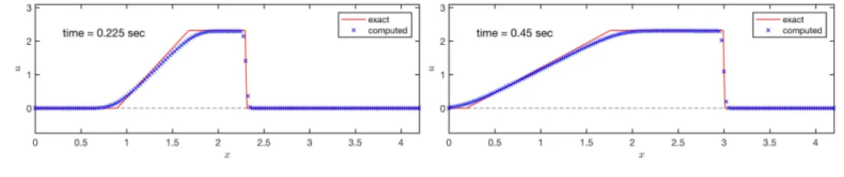
Dam break flow : Riterr’s exact solution . The initial condition for the Ritter’s test is defined with
hL= 1.0 m and hR= 0.0 m .
This is an initial condition with a dry-land on the right-hand side. The exact solution is composed of a left going rarefaction wave that is a concave parabola connecting the constant water depth hL and the dry zone (hR = 0). This parabola covers the range [xA(t), xB(t)], extending with
xA(t) = x0 tpghL and xB(t) = x0+ 2tpghL. Hence, the evolution of the depth’s distribution
reads (e.g. [32] or [33]) h(x, y, t) = 8 > > > > < > > > > : hL for x xA(t) , 4 9g ⇣p ghL x x2t0 ⌘2 for xA(t) < x < xB(t) , 0.0 for xB(t) x , (32)
for the flow depth, where the corresponding velocity is linearly distributed in the rarefaction
u(x, y, t) = 8 > > > > < > > > > : 0.0 for x xA(t) , 2 3 ⇣p ghL+x xt 0 ⌘ for xA(t) < x < xB(t) , 0.0 for xB(t) x . (33)
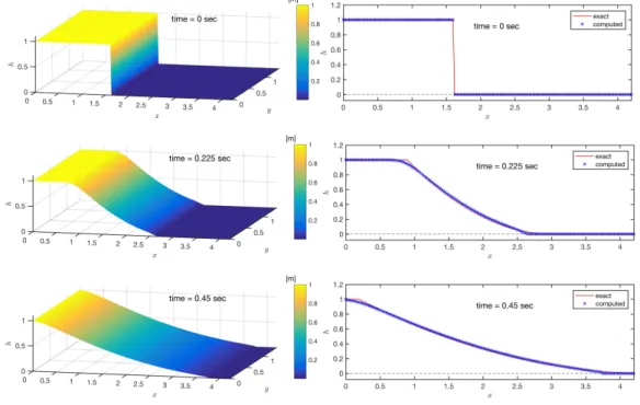
Here we recall that h(x, y, t) is uniformly distributed in the lateral y-direction. The computed depth
130
distributions are respectively shown in Fig. 4 at t = 0.0, 0.225 and 0.45 s, where the corresponding section views along the central line (y = 0.7) are shown in the right panels. In the right panels of Fig. 4, the blue “⇥” markers denote the computed results and the analytical solutions are depicted by red lines. The computed results demonstrate the capability of present approach of adequately describing this dam break problem.
135
Dam break flow : Stoker’s exact solution . The initial condition for the Stoker’s test is defined with
Figure 4: The depth evolution in the dry land case — Ritter’s solution.
Then, the exact solution is composed by a left-going rarefaction wave connecting the initial left depth hL to a constant non-vanishing depth hM by a concave parabola, and at the right end of
the constant depth hM a right-going shock that relates hM and hR. The parabola ranges from
xA(t) = x0 tpghL to xB(t) = x0+ t uM pghM , and the zone of constant depth lies in
[xB(t), xC(t)]. Position xC(t) denotes the location of the shock wave moving with a constant
velocity ushock. The derivation of this Stoker’s solution is tedious, so we just list the results and
refer the readers to e.g. [32] for details. The velocity ushockis the solution of
4⇣4⇧A1/2+ 1⌘u2 shock 8 p ghLushock ghR⇧A= 0 with ⇧A= 1 + 1 + 8u2shock/(ghR) 1/2
. Once the shock velocity ushockis determined, the thickness
of the bore hM and the value of uM can be determined by the relations ghM = 4u2shock/⇧A, and
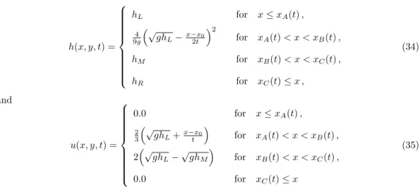
h(x, y, t) = 8 > > > > > > > > < > > > > > > > > : hL for x xA(t) , 4 9g ⇣p ghL x x2t0 ⌘2 for xA(t) < x < xB(t) , hM for xB(t) < x < xC(t) , hR for xC(t) x , (34) and u(x, y, t) = 8 > > > > > > > > < > > > > > > > > : 0.0 for x xA(t) , 2 3 ⇣p ghL+x xt 0 ⌘ for xA(t) < x < xB(t) , 2⇣pghL pghM ⌘ for xB(t) < x < xC(t) , 0.0 for xC(t) x (35)
represents the corresponding velocity distribution.
Figure 5: The depth evolution in the wet land case — Stoker’s solution
velocity, as shown in Figs. 5 and 6, respectively. Similar to the illustration in Fig. 4, the red lines represent the analytical solutions and the computed ones are denoted by blue cross-markers “⇥”.
Figure 6: The velocity distributions in the wet land case — Stoker’s solution
For both dam-break problems considered in this section, the numerical solutions fit well with
140
the exact solutions. Mesh convergence has been performed and optimal convergence of first order is achived for these non smooth exact solutions, even if no special treatment is performed at the wet-dry moving boundary.
3.2. Quasi-1D flows on inclined flat plane : Parabolic Similarity solution
One particular similarity solution in the one-dimensional case was proposed in [34] and has been generalized in [35], where a finite mass of granular material slides along a flat plane keeping the depth distribution in a parabolic shape along the down-slope direction. In this example, a flat plane with inclination angle ✓c = 35 is considered, on which a local coordinate system O⇠⌘⇣ is
assigned with the ⇠-axis pointing towards the down-slope direction, the ⌘-axis towards the cross-slope direction and the ⇣-axis pointing upwards normal to the plane. With respect to the multi-scale approximation proposed in Sect. 2, this inclined flat plane serves as the topography, i.e., z = b(x, y), over the horizontal xy-plane
b(x, y) = (xR x) tan ✓c with (x, y)2 ⌦ .
Here, a rectangular domain ⌦ = [0, 4.2 m]⇥ [0, 1.4 m] and a “structured” triangular mesh of 169 ⇤ 57
145
vertices and 11816 triangular elemnts are employed.
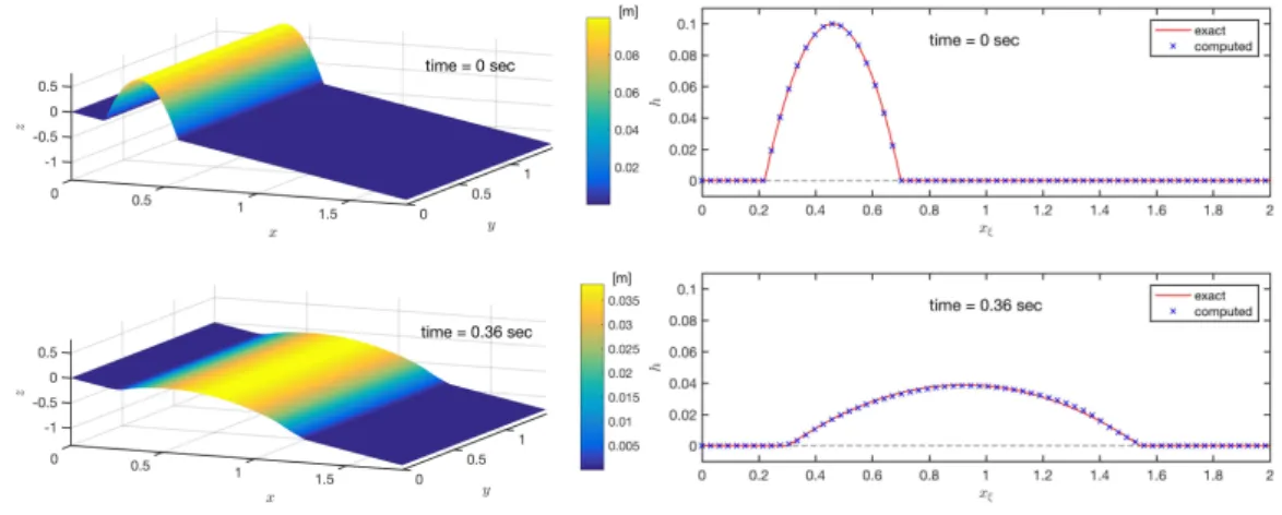
In the coordinate system O⇠⌘⇣, the initial depth is uniform in ⌘-direction and exhibits a parabolic
shape along the down-slope ⇠-direction, namely
h(⇠, ⌘, t = 0) = 8 > < > : h0 ✓ 1.0 ⇣⇠ 0.460.24 ⌘2 ◆ for |⇠ 0.46| 0.24 , 0.0 elsewhere , (36)
where the flow thickness h is measured normal to the plane and h0= 0.1 m is the maximum depth
located at ⇠ = 0.46. For the initial velocity (u⇠, v⌘) tangential to the flat plane, a linear distribution
of velocity in the down-slope direction is assigned to the moving body, whilst no speed is given in the lateral direction. That is,
u⇠(⇠, ⌘, t = 0) = 8 > < > : u⇠c ⇣ 1.0 + 0.4⇣⇠ 0.460.24 ⌘⌘ for |⇠ 0.46| 0.24 , 0.0 elsewhere , v⌘(⇠, ⌘, t = 0) = 0.0 , (37)
where u⇠c= 0.8 m/s is the initial velocity of the center of the parabilic moving mass.
In the computation, the so-called earth-pressure coefficient introduced in [35] is set to be unity, so that the center of the moving mass slides with velocity
ucenter⇠ (t) = u⇠c+
Z t 0
g sin ✓c µ cos ✓c dt0, (38)
in which µ is the Coulomb friction coefficient as introduced in (27). As time increases, the moving body extends with respect to the center symmetrically, keeping the parabolic shape and a linear distribution for velocity along the down-slope direction (⇠-direction). Since the total mass should
150
be conserved, the moving body becomes flatter and flatter as it extends. Figure 7 illustrates the depth distributions at t = 0.0 and 0.36 s, respectively. The corresponding section views along the central line (y = 0.7) are shown in the right panels, in which the red lines represent the analytical solutions and the blue “⇥” markers denote the numerical predictions.
Figure 7: The depth evolution in the case of the similarity solution.
Dam break flow over wet land — Stoker’s solution
155
3.3. Parabolic Similarity Solution
4. Application to Back-Calculation of a Real Event
The proposed method is further applied to back-calculation of a real event, the Hsiaolin landslide, which took place during the typhoon Morakot in August 2009. Within 72 hours, an abnormal heavy rainfall of more than 2,000 mm accumulated precipitation triggered a large-scale landslide and the
160
subsequent debris flow attached and buried the Hsiaolin village in southern Taiwan. It is reported that there were more than 470 victims in this event (see e.g. [13, 36]). The post-disaster field investigation indicates that the major landslide body had an extent of 57⇥ 104m2 with a mean
depth of 42± 3 m (see [37]).
In our application, the computational domain covers an area of 3,700 m⇥ 2,210 m with 371⇥222
165
vertices and 163, 540 triangle elements in total. The applied angle of basal friction is set at 12.5 . Figure 8 shows the evolution of the flow thickness at sequential time levels, where the dark brown color indicates the scoured area at the corresponding time level. The mass is released from rest, as employed in [13] and shown in the panel at t = 0 sec, where the thick red line marks the area of Hsiaolin village. Approximately at the center of the figure stands a ridge, the 590 Height marked
170
by a red star marker, which is capable of protecting the village when the amount of the moving mass is not too large. At t = 30 sec, the moving mass accumulates in front of the 590 Height and
Figure 8: Evolution of the flow thickness, where the area covered by the dark brown color indicates the scoured area at the corresponding time level.
exhibits high flow depth. Due to the abnormally huge volume, part of the moving mass flows over the hill and towards the village (see the panel at t = 60 sec). One can recognize that there are approximately three branches: the northern branch, the middle main stream and the southern one.
175
At this time level, the debris just touches the village, while the northern and middle ones have arrived at the river channel. At t = 90 sec, the material slows down and begins to deposit, while the main stream collects most of the material and only a small part goes through the village. After
Figure 9: Velocity distributions of the moving mass at sequential time levels, as shown in Fig. 8.
t = 120 sec, the majority of the material has come to rest, and as a consequence, the distribution of flow thickness does not significantly change from t = 120 to t = 150 sec.
180
The corresponding velocity (speed) distributions with respect to Fig. 8 are illustrated in Fig. 9. At t = 0, the moving mass is released from rest. The 590 Height retards the moving debris, so that significant velocity reduction can be found behind the ridge, see the the panel for t = 30 sec. The flow front begins to deposit once it crosses the river channel and touches the river bank (t = 60 sec), while the highest speed reaches 60 m/s. From t = 90 sec to t = 150 sec, the speed generally
corresponds to the local slope, and the material at the downstream area comes nearly to rest.
Figure 10: The satllite image taken approximately 5 months after the event.
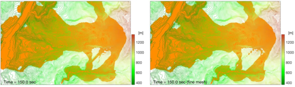
Figure 11: The computed scoured area. Left: coarse mesh; Right: finer mesh.
Figure 10 is a satellite image taken ca. 5 months after the event, where the bare area approx-imately depicts the flow paths, including the source scar and deposit area. The right panel of Fig. 10 illustrates the flow-impacted area during the computation of Fig. 8, and Fig. 11 shows the flow-covered area computed with finer mesh (double of vertices), where no significant discrepancy
190
is recognized. It reveals that the solution converges with mesh-refinement. Comparing the flow impact area (from t = 0 to t = 150 sec with 6 sec increment) with the satellite image, the computed results cover a slightly larger area than that in the satellite image. Especially at the northern and southern flanks of the source area, more mass slides sidewise and over the ridges. This overflow is
suspected to be caused by the initial condition, in which the whole mass is suddenly released.
195
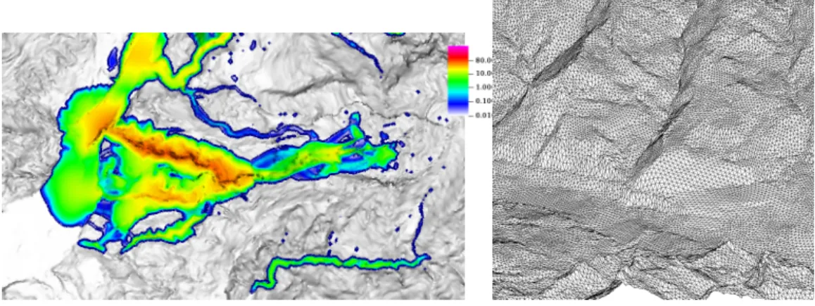
Figure 12: The numerical results at time t = 150 sec with structured triangular mesh. Left: the flow thickness; Right: Zoom on the mesh.
Figure 13: The numerical results at time t = 150 sec with unstructured triangular mesh (obtained by interpolation). Left: the flow thickness; Right: Zoom on the mesh.
The present approach is also suitable for unstructured mesh. Figure 12 shows the flow thickness (left panel) at time t = 150 sec with structured triangular mesh, where the zoomed mesh pattern is shown in the right panel. The distribution of the flow thickness at t = 150 sec and the employed unstructured mesh are illustrated in Fig. 13, where the topography and initial depth are obtained by interpolation with repect to the data used in computation for Figs. 8 and 9. In both Figs. 12
and 13, the margin indicates the location of flow thickness of 1 cm. Although discrepancy of the margin locations can be identified, the distribution of the material are rather similar. In fact, even if the interpolated topography is globally similar to the initial one, there are locally some di↵erence that can explain the shifting in the computed wave front. However, the global shapes are similar.
5. Concluding remarks
205
In the present study we have proposed a multi-scale approach for describing the dynamic be-haviors of shallow flows over complex topographies. Since the topographic surface is of non-trivial geometry, it is always impossible to defined a non singular mapping that fit every where with the basal surface. Then derivation of a global depth average is questionable. We have proposed a numerical strategy that can be view as a 3D finite volume approximation of the free surface
in-210
compressible Naviers-Stokes equations. Locally there is a single volume in the normal direction to the basal surface. This dynamic 3D volume is defined by a surface cell fitting with the basal and a average depth. The cell surface is obtained in the framework of vertex-centered with unstructured mesh of flat triangles. The depth of the 3D volume is an unknown of the problem. Therefore, depth average is achieved locally in the numerical approximation. The final numerical scheme is based
215
on computations of fluxes according to approximated solution of Riemann problems. For simple basal surface, we have recover the solution of classical discretization of the Shallow water equations with optimal rate of convergence to the exact solution. The application to the large-scale event, the Hsiaolin landslide, shows that the numerical computation reasonably retraces the landslide paths and deposit, where sound agreements can be identified with respect to the satellite picture and
220
in-situ measurement. Unstructured mesh framework had some high potential for engineering appli-cations as it provide more flexibility in the representation of the topography. In this context, it is more easy and useful to develop local refinement based on some specific criteria such as curvature or geological properties.
Although the results have shown the general applicability of the present approach, it should
225
be noted that it follows the depth-averaged concept, so that some important e↵ects or phenom-ena are neglected or still missing. For example, the non-uniform distribution of velocity along the flow thickness is not taken into account yet. In experiments of geophysical mass flows, either for dry granular flows or for saturated grain-fluid debris flows where the impact of the viscosity is significant, the velocity profiles are generally non-uniform [38, 39]. This non-uniformity
troduces the correction (shape) factor ( 1) induced by the advective terms in the momentum equations, while the non-unity value of the correction factor will change the characteristic struc-ture of the equation system ([40]), so that additional treatment is needed. Another issue is the non-hydrostatic pressure, which could be induced by the non-uniform velocity profile [38, 24, 25], grain-size-distribution [41], or the so-called enhanced gravity (excess pore fluid pressure induced by
235
granular dilatancy) [42, 15, 43, 44, 41]. These neglected phenomena might explain the employment of a small angle of basal friction in our back-calculation for the Hsiaolin event. And a two-phase model might be the plausible solution, but more parameters would be needed in the model. As well, the erosion and deposition should be integrated into the numerical model for a more realistic scenario, where the determination of the evolution of the mesh system would play the crucial role.
240
More e↵orts are requested on these tasks and we will report on the future results in due time.
Acknowledgement
Part of the results were conducted during the visit of J. Vides and B. Nkonga to the Department of Hydraulics and Ocean Engineering, NCKU, Taiwan, and the visit of Y.C. Tai and C.Y. Kuo to the University of Nice Cˆote d’Azur (UCA) in the frame work of the Inria-MOST Associate team program
245
AMoSS and funding MOST-105-2911-I-006-502. B. Nkonga acknowledges the warm hospitality of the NCTS at NTU Taipei. Y.C. Tai was partially supported by MOST 106-2221-E-006-056.
Appendix
A.1. Surface Integrals
In order to derive the finite volume scheme, we need to be able to compute integrals over the boundary @Ve i of the form Z Ve i r · uuu dexxx = Z @Ve i u uu· nnn dSxexx and Z Ve i r · TTT dexxx = Z @Ve i T TTnnn dSexxx, (A.1)
with TTT = uuu⌦ uuu + PPP. Recall thatxxx are Cartesian coordinates; ne nn is the outward unit normal vector
250
in this system of coordinates and dSexxx is the surface increment.
In this context, it is more convenient to use a local surface coordinate in the evaluation of the fluxes (A.1). Thus, the transformation (2) will be used, which we recall here below:
e x
xx⇣e⇠⇠⇠⌘= ⇠ ggg⇠+ ⌘ ggg⌘+ ⇣ ggg⇣,
where ggg⇠, ggg⌘ and ggg⇣ are the basis vectors of the local coordinate and e⇠⇠⇠ = (⇠, ⌘, ⇣)t, so that the
stress tensor reads
TTT = T⇠⇠ggg⇠⌦ ggg⇠+ T⇠⌘ggg⇠⌦ ggg⌘+ T⇠⇣ggg⇠⌦ ggg⇣
+ T⌘⇠ggg⌘⌦ ggg⇠+ T⌘⌘ggg⌘⌦ ggg⌘+ T⌘⇣ggg⌘⌦ ggg⇣
+ T⇣⇠ggg⇣⌦ ggg⇠+ T⇣⌘ggg⇣⌦ ggg⌘+ T⇣⇣ggg⇣⌦ ggg⇣.
We also urge the reader to recall that the Jacobian of the transformation is j = (ggg⇠⇥ ggg⌘)· ggg⇣, as
was introduced in (3). Let us now compute the integrals (A.1) on three di↵erent types of surfaces: basal, flow and side surfaces.
On Basal Surfaces
255
In this case, the surface is only parametrized by ⇠ and ⌘, andxexx⇣e⇠⇠⇠⌘= ⇠ ggg⇠+ ⌘ ggg⌘. First, for the
continuity equation, we get Z Ce i uuu· nnn dSexxx= Z ⇠ Z ⌘ u u u· ✓ @exxx @⇠ d⇠⇥ @exxx @⌘d⌘ ◆ = Z ⇠ Z ⌘ u u u· (ggg⇠d⇠⇥ ggg⌘d⌘) = Z ⇠ Z ⌘ u⇣ggg⇣· (ggg⇠d⇠⇥ ggg⌘d⌘) = Z ⇠ Z ⌘ j u⇣d⇠d⌘ and aei = Z ⇠ Z ⌘ ggg⇠⇥ ggg⌘ kggg⇠⇥ ggg⌘k· (ggg⇠d⇠⇥ ggg⌘d⌘) = Z ⇠ Z ⌘ ggg⇣· (ggg⇠d⇠⇥ ggg⌘d⌘) = Z ⇠ Z ⌘ jd⇠d⌘ ,
where ae
i = j/6 for the triangular shape of the local element. Then, for the momentum equation,
the associated integral reads Z Ce i T T TnnndSxxex= Z ⇠ Z ⌘ T TT (ggg⇠d⇠⇥ ggg⌘d⌘) = Z ⇠ Z ⌘ T T T (ggg⇠⇥ ggg⌘) d⇠d⌘ = Z ⇠ Z ⌘ j TTTggg⇣d⇠d⌘ . On Flow Surfaces
Here, the surface is parametrized by ⇠ and ⌘: xexx⇣e⇠⇠⇠⌘ = ⇠ ggg⇠ + ⌘ ggg⌘+ h (t, ⇠, ⌘) ggg⇣. Thus, the
surface integral associated to the continuity equation becomes Z Ce i uuu· nnn dSexxx= Z ⇠ Z ⌘ u uu· ✓ @xxex @⇠ d⇠⇥ @xxex @⌘d⌘ ◆ = Z ⇠ Z ⌘ u uu· ((ggg⇠+ @⇠h ggg⇣) d⇠⇥ (ggg⌘+ @⌘h ggg⇣) d⌘) = Z ⇠ Z ⌘ u uu· (ggg⇠⇥ ggg⌘+ @⌘h ggg⇠⇥ ggg⇣+ @⇠h ggg⇣⇥ ggg⌘) d⇠d⌘ = Z ⇠ Z ⌘ juuu· ggg⇣ @ ⌘h ggg⌘ @⇠h ggg⇠ d⇠d⌘ = Z ⇠ Z ⌘ u⇣ @⇠h u⇠ @⌘h u⌘ j d⇠d⌘,
where the relations ggg⇠= 1
j(ggg⌘⇥ ggg⇣), ggg⌘= 1
j(ggg⇣⇥ ggg⇠) and ggg⇣= ggg⇣= 1
j(ggg⇠⇥ ggg⌘) have appropriately
been used. In addition, the momentum equation yields Z Ce i T T Tnnn dSxexx= Z ⇠ Z ⌘ T TT (ggg⇠⇥ ggg⌘+ @⌘h ggg⇠⇥ ggg⇣+ @⇠h ggg⇣⇥ ggg⌘) d⇠d⌘ = Z ⇠ Z ⌘ j TTT ggg⇣ @⌘h ggg⌘ @⇠h ggg⇠ d⇠d⌘ . On Side Surfaces
In this last case, the surface is parametrized by ` and ⇣. Specifically, we have e
with ↵⇠ and ↵⌘being two constants. Then, the surface integral over @Vie\ @Vme is Z @Ve i\@Vme u u u· nnn dSxxex= Z ` Z ⇣ u u u· ✓ @ @`xxexd`⇥ @ @⇣xxxd⇣e ◆ = Z ` Z ⇣ u u u·h(↵⇠ggg⇠+ ↵⌘ggg⌘)⇥ ggg⇣ i d`d⇣ = Z ` Z ⇣ u u u·h↵⇠(ggg⇠⇥ ggg⇣) + ↵⌘(ggg⌘⇥ ggg⇣) i d`d⇣ = Z ` Z ⇣ juuu·⇣ ↵⇠ggg⌘+ ↵⌘ggg⇠ ⌘ d`d⇣ = Z ` Z ⇣ juuu· ennn d`d⇣ = Z ` Z ⇣ j⇣u⇠ggg ⇠· ennn + u⌘ggg⌘· ennn ⌘ d`d⇣ ,
where the normal vectorennn = ↵⇠ggg⌘+ ↵⌘ggg⇠= ggg⌘· ennn ggg⌘+ggg⇠· ennn ggg⇠, with ↵⇠= ggg⌘· ennn and ↵⌘= ggg⇠· ennn.
Proceeding in the same way, we get, for any tensor TTT , Z @Ve i\@Vme T T T nnn dSexxx= Z ` Z ⇣ j TTTnnen d`d⇣ = Z ` Z ⇣ j ggg⇠· ennn TTT ggg⇠+ ggg⌘· ennn TTT ggg⌘ d`d⇣ .
A.2. Interface Normal Vectors on a Triangular Element
In practice, we have plane surfaces as the normal vectors are constant and formulations with the covariant vectors are straightforward.
260
Let us consider a given element defined by the pointsxexxi,xxexj andexxxk, oriented as in Figure 14.
In order to obtain a finite volume approximation, we need to be able to define cell interface normal vectors. For this, on the considered triangular element, we first introduce the midpoints
e xxxij=ex x xi+xexxj 2 , xxexjk= e xxxj+xexxk 2 , xxexki= e x xxk+xxexi 2 , and the triangle’s centroid
e x x xg =e x x xi+xexxj+xxexk 3 , so that the integrated normal vectors are given by
8 > > > > > > < > > > > > > : neij= Z `ij jennnd` = ⇣xexxg xxxeij ⌘ ⇥ ggg⇣, ne jk= Z `jk jnnnd`e = ⇣xexxg xxxejk ⌘ ⇥ ggg⇣, neki= Z `ki jennnd` = ⇣xexxg xxxeki ⌘ ⇥ ggg⇣,
y x e x xxg e xxxi e x xxk e x x xj ne ki ne jk ne ij e x xxjk e x x xki e x x xij
Figure 14: Integrated normal vectors on a triangular element.
where e x x xg xxexij = 1 6 ⇣ e x x xi xexxj+ 2exxxk ⌘ =1 6 ⇣ 2(exxxk xexxi) (exxxj xexxi) ⌘ = ggg⇠+ 2ggg⌘ 6 , e x x xg xxexjk= 1 6 ⇣ e x x xj exxxk+ 2exxxi ⌘ =1 6 ⇣ (exxxk xexxi) (exxxj xexxi) ⌘ = ggg⇠ ggg⌘ 6 , e x x xg xxexki= 1 6 ⇣ e xxxk xexxi+ 2exxxj ⌘ =1 6 ⇣ (exxxk xxexi) + 2(exxxj exxxi) ⌘ = 2ggg⇠ ggg⌘ 6 .
A relation that will be useful to derive simplified expressions for the above mentioned normal vectors is (↵⌘ggg⌘+ ↵⇠ggg⇠)⇥ ggg⇣ = 1j(↵⌘ggg⌘+ ↵⇠ggg⇠)⇥ (ggg⇠⇥ ggg⌘) = 1j(↵⇠ggg⇠· ggg⌘+ ↵⌘ggg⌘· ggg⌘) ggg⇠ 1j(↵⌘ggg⇠· ggg⌘+ ↵⇠ggg⇠· ggg⇠) ggg⌘ = 1 j h (↵⇠ggg⇠· ggg⌘+ ↵⌘ggg⌘· ggg⌘) ggg⇠ (↵⌘ggg⇠· ggg⌘+ ↵⇠ggg⇠· ggg⇠) ggg⌘ i .
having recalled equation (3). Finally, the normal vectors are formulated in the following way: ne ij= ( 2 ggg⌘ ggg⇠) 6 ⇥ ggg⇣= ( ggg⇠· ggg⌘ 2ggg⌘· ggg⌘) ggg⇠+ ( 2 ggg⇠· ggg⌘ ggg⇠· ggg⇠) ggg⌘ 6j , ne jk= ( ggg⌘ ggg⇠) 6 ⇥ ggg⇣= ( ggg⇠· ggg⌘+ ggg⌘· ggg⌘) ggg⇠ ( ggg⇠· ggg⌘+ ggg⇠· ggg⇠) ggg⌘ 6j , neki= ( ggg⌘+ 2ggg⇠) 6 ⇥ ggg⇣ = ( 2ggg⇠· ggg⌘+ ggg⌘· ggg⌘) ggg⇠+ ( ggg⇠· ggg⌘+ 2ggg⇠· ggg⇠) ggg⌘ 6j . References
[1] S. Savage, K. Hutter, The dynamics of avalanches of granular materials from initiation to runout. Part I: Analysis, Acta Mechanica 86 (1-4) (1991) 201–223.
[2] R. Greve, T. Koch, K. Hutter, Unconfined flow of granular avalanches along a partly curved surface. I. Theory, Proceedings of the Royal Society of London. Series A: Mathematical and
265
Physical Sciences 445 (1924) (1994) 399–413.
[3] J. Gray, M. Wieland, K. Hutter, Gravity-driven free surface flow of granular avalanches over complex basal topography, Proc. R. Soc. Lond. A 455 (1999) 1841–1875.
[4] J. M. N. T. Gray, Y.-C. Tai, S. Noelle, Shock waves, dead zones and particle-free regions in rapid granular free-surface flows, Journal of Fluid Mechanics 491 (2003) 161–181.
270
[5] X. Meng, Y. Wang, Modelling and numerical simulation of two-phase debris flows, Acta Geotechnica 11 (5) (2016) 1027–1045.
[6] S. P. Pudasaini, K. Hutter, Rapid shear flows of dry granular masses down curved and twisted channels, Journal of Fluid Mechanics 495 (2003) 193–208.
[7] F. Bouchut, M. Westdickenberg, Gravity driven shallow water models for arbitrary topography,
275
Comm. Math. Sci 2 (2004) 359–389.
[8] W. Hui, P. Li, Z. Li, A unified coordinate system for solving the two-dimensional Euler equa-tions, Journal of Computational Physics 153 (2) (1999) 596–637.
[9] W. H. Hui, The unified coordinate system in computational fluid dynamics, Communications in Computational Physics 2 (4) (2007) 577–610.
[10] I. Luca, Y.-C. Tai, C.-Y. Kuo, et al., Shallow geophysical mass flows down arbitrary topography, Springer, 2016.
[11] Y.-C. Tai, C.-Y. Kuo, Modelling shallow debris flows of the Coulomb-mixture type over tempo-rally varying topography, Natural Hazards and Earth System Sciences 12 (2) (2012) 269–280. [12] Y.-C. Tai, C.-Y. Kuo, W.-H. Hui, An alternative depth-integrated formulation for granular
285
avalanches over temporally varying topography with small curvature, Geophysical & Astro-physical Fluid Dynamics 106 (6) (2012) 596 – 629.
[13] C. Kuo, Y. Tai, C. Chen, K. Chang, A. Siau, J. Dong, R. Han, T. Shimamoto, C. Lee, The landslide stage of the Hsiaolin catastrophe: Simulation and validation, Journal of Geophysical Research: Earth Surface 116 (F04007) (2011) doi:10.1029/ 2010JF001921.
290
[14] Y.-C. Tai, J. Heß, Y. Wang, Modeling two-phase debris flows with grain-fluid separation over rugged topography: Application to the 2009 Hsiaolin event, Taiwan, Journal of Geophysical Research: Earth Surface 124 (2) (2019) 305–333.
[15] R. M. Iverson, Regulation of landslide motion by dilatancy and pore pressure feedback, Journal of Geophysical Research: Earth Surface 110 (F2).
295
[16] J. Heß, Y. Wang, K. Hutter, Thermodynamically consistent modeling of granular-fluid mixtures incorporating pore pressure evolution and hypoplastic behavior, Continuum Mechanics and Thermodynamics 29 (1) (2017) 311–343.
[17] J. Heß, Y.-C. Tai, Y. Wang, Debris flows with pore pressure and intergranular friction on rugged topography, Computers & Fluids 190 (2019) 139–155.
300
[18] B. Braconnier, J.-J. Hu, Y.-Y. Niu, B. Nkonga, K.-M. Shyue, Numerical simulations of low Mach compressible two-phase flows: Preliminary assessment of some basic solution techniques., ESAIM: Proc. 28 (2009) 117–134.
[19] C.-Y. Kuo, B. Nkonga, M. Ricchiuto, Y.-C. Tai, B. Braconnier., Dry granular flows with erosion/deposition process., ESAIM: Proc. 28 (2009) 135–149.
305
[20] C. Juez, D. Caviedes-Voulli`eme, J. Murillo, P. Garc´ıa-Navarro, 2D dry granular free-surface transient flow over complex topography with obstacles. Part II: Numerical predictions of fluid structures and benchmarking, Computers & Geosciences 73 (0) (2014) 142 – 163.
[21] C. Kuo, Y. Tai, F. Bouchut, A. Mangeney, M. Pelanti, R. Chen, K. Chang, Simulation of Tsaol-ing landslide, Taiwan, based on Saint Venant equations over general topography, EngineerTsaol-ing
310
Geology 104 (3-4) (2009) 181 – 189.
[22] M. Quecedo, M. Pastor, Finite element modelling of free surface flows on inclined and curved beds, Journal of Computational Physics 189 (1) (2003) 45 – 62.
[23] E. Audusse, M. Bristeau, A well-balanced positivity preserving second-order scheme for shallow water flows on unstructured meshes, Journal of Computational Physics 206 (1) (2005) 311 –
315
333.
[24] G. Richard, S. Gavrilyuk, A new model of roll waves: comparison with Brock’s experiments, Journal of Fluid Mechanics 698 (2012) 374–405.
[25] G. Richard, S. Gavrilyuk, The classical hydraulic jump in a model of shear shallow-water flows, Journal of Fluid Mechanics (2013) 492–521.
320
[26] A. Bhole, B. Nkonga, S. Gavrilyuk, K. Ivanova, Fluctuation splitting riemann solver for a non-conservative modeling of shear shallow water flow, Journal of Computational Physics 392 (2019) 205–226.
[27] S. Savage, K. Hutter, The motion of a finite mass of granular material down a rough incline, J. Fluid Mech. 199 (1989) 177–215.
325
[28] O. Pouliquen, Y. Forterre, Friction law for dense granular flows: Application to the motion of mass down a rough inclined plane., J. Fluid Mech. 453 (2002) 133–151.
[29] G. Midi, On dense granular flows., Eur. Phys. J. E 14.
[30] G. Taubin, Estimating the tensor of curvature of a surface from a polyhedral approximation, Proceedings, Fifth International Conference on Computer Vision (1995) 902–907.
330
[31] E. Audusse, F. Bouchut, M. Bristeau, R. Klein, B. Perthame, A fast and stable well-balanced scheme with hydrostatic reconstruction for shallow water flows, SIAM J. Sci. Comput. 25 (2004) 2050–2065.
[32] J. J. Stoker, Water waves: The mathematical theory with applications, Vol. IV of Pure and applied mathematics, Interscience Publishers, Inc., New York, 1957.
[33] O. Delestre, C. Lucas, P.-A. Ksinant, F. Darboux, C. Laguerre, T.-N. Vo, F. James, S. Cordier, et al., Swashes: a compilation of shallow water analytic solutions for hydraulic and environ-mental studies, International Journal for Numerical Methods in Fluids 72 (3) (2013) 269–300. [34] S. B. Savage, K. Hutter, The motion of a finite mass of granular material down a rough incline,
Journal of fluid mechanics 199 (1989) 177–215.
340
[35] Y.-C. Tai, S. Noelle, J. Gray, K. Hutter, Shock-capturing and front-tracking methods for granular avalanches, Journal of Computational Physics 175 (1) (2002) 269–301.
[36] Y. Kuo, Y. Tsai, Y. Chen, C. Shieh, K. Miyamoto, T. Itoh, Movement of deep-seated rainfall-induced landslide at shiao lin village during typhoon morakot, Landslides 10 (2) (2013) 191–202. [37] J. Dong, Y. Li, C. Kuo, R. Sung, M. Li, C. Lee, C. Chen, W. Lee, The formation and breach
345
of a short-lived landslide dam at Hsiaolin village, taiwan part I: post-event reconstruction of dam geometry, Engineering Geology 123 (1) (2011) 40–59.
[38] O. Castro-Orgaz, K. Hutter, J. V. Giraldez, W. H. Hager, Nonhydrostatic granular flow over 3-d terrain: New boussinesq-type gravity waves?, Journal of Geophysical Research: Earth Surface 120 (1) (2015) 1–28.
350
[39] R. Kaitna, W. Dietrich, L. Hsu, Surface slopes, velocity profiles and fluid pressure in coarse-grained debris flows saturated with water and mud, Journal of Fluid Mechanics 741 (2014) 377–403.
[40] P.-Y. Lagr´ee, G. Saingier, S. Deboeuf, L. Staron, S. Popinet, Granular front for flow down a rough incline: about the value of the shape factor in depths averaged models, in: EPJ Web of
355
Conferences, Vol. 140, EDP Sciences, 2017, p. 03046.
[41] R. Kaitna, M. C. Palucis, B. Yohannes, K. M. Hill, W. E. Dietrich, E↵ects of coarse grain size distribution and fine particle content on pore fluid pressure and shear behavior in experimental debris flows, Journal of Geophysical Research: Earth Surface 121 (2) (2016) 415–441. [42] R. P. Denlinger, R. M. Iverson, Granular avalanches across irregular three-dimensional terrain:
360