HAL Id: tel-02271260
https://tel.archives-ouvertes.fr/tel-02271260
Submitted on 26 Aug 2019
HAL is a multi-disciplinary open access
archive for the deposit and dissemination of sci-entific research documents, whether they are pub-lished or not. The documents may come from teaching and research institutions in France or abroad, or from public or private research centers.
L’archive ouverte pluridisciplinaire HAL, est destinée au dépôt et à la diffusion de documents scientifiques de niveau recherche, publiés ou non, émanant des établissements d’enseignement et de recherche français ou étrangers, des laboratoires publics ou privés.
New nested grids technique for 2D shallow water
equations
Huda Altaie
To cite this version:
Huda Altaie. New nested grids technique for 2D shallow water equations. Numerical Analysis [math.NA]. Université Côte d’Azur, 2018. English. �NNT : 2018AZUR4220�. �tel-02271260�
Nouvelle Technique de Grilles Imbriquées pour les équations de
Saint-Venant 2D
New Nested Grids
Technique
For 2D Shallow Water Equations
Huda Omran ALTAIE
Laboratoire Jean Alexandre Dieudonné LJAD
Présentée en vue de l'obtentiondu grade de docteur en Science
Mathématiques de l'Université cote d'Azur
Dirigée par : Fabrice Planchon / Pierre Dreyfuss
Soutenue le : 17/12 2018
Devant le jury, composé de :
Xavier Antoine,Professeur- Université de Lorraine, Rapporteur
Stéphane Clain,Associate Professeur HDR- Université de Minho (Portugal), Rapporteur
Isabelle Gallagher, Professeur- Ecole Normale Supérieure de Paris, Examinatrice
Marjolaine Puel, Professeur- Université Nice Sophia-Antipolis, Examinatrice
Fabrice Planchon, Professeur-Université Nice Sophia-Antipolis, Directeur de thèse
Pierre Dreyfuss, Maître de conférences-Université Nice Sophia-Antipolis, Co-Directeur de thèse
ABSTRACT
Most flows in the rivers, seas, and ocean are shallow water flow in which the horizontal length and velocity scales are much larger than the vertical ones. The mathematical formulation of these flows, so-called shallow water equations (SWEs). These equations are a system of hyperbolic partial differential equations and they are effective for many physical phenomena in the oceans, coastal regions, rivers and canals.
This thesis focuses on the design of a new two-way interaction technique for multiple nested grids 2DSWEs using the numerical methods. The first part of this thesis includes, proposing several ways to develop the derivation of shallow water model. The complete derivation of this system from Navier-Stokes equations is explained. Studying the development and evaluation of numerical methods by suggesting new spatial and temporal discretization techniques in a standard C-grid using an explicit finite difference method in space and leapfrog with Robert-Asselin filter in time which are effective for modeling in oceanic and atmospheric flows. Several numerical examples for this model using Gaussian level initial condition are implemented in order to validate the efficiency of the proposed method.
In the second part of our work, we are interested to propose a new two-way interaction technique for multiple nested grids to solve ocean models using four choices of higher restriction operators (update schemes) for the free surface elevation and velocities with high accuracy results. Our work focused on the numerical resolution of SWEs by nested grids. At each level of resolution, we used explicit finite differences methods on Arakawa C-grid. In order to be able to refine the calculations in troubled regions and move them into quiet areas, we have considered several levels of resolution using nested grids. This makes it possible to considerably increase the performance ratio of the method, provided that the interactions (spatial and temporal) between the grids are effectively controlled.
In the third part of this thesis, several numerical examples are tested to show and verify two-way interaction technique for multiple nested grids of shallow water models can works efficiently over different periods of time with nesting 3:1 and 5:1 at multiple levels. Some examples for multiple nested grids of the tsunami model with nesting 5:1 using moving boundary conditions are tested in the fourth part of this work.
Keywords: Nested grid, One-way nesting, Two-way nesting, Mesh refinement, Explicit finite difference method, Shallow water model, Derivation of 2D shallow water equations, Ocean model, Boundary conditions, Optimum feedback, Free surface flows, Hydrostatic pressure, Coastal regions, Incompressible fluid, Fluid dynamics, Tsunami deposit, Tsunami hazards, Dynamical interface.
Acknowledgment
First and foremost, I would like to express my sincere gratitude to my supervisors Prof. Fabrice Planchon and Mr.Pierre Dreyfuss for the continuous support of my Ph.D. study and research, for their patience, motivation, enthusiasm, and immense knowledge. Their guidance helped me in all the time of research and writing of this thesis. Also, for their confidence and constant encouragement, for their enthusiasm, for their many tips. I could not have imagined having excellent supervisors and mentors for my Ph.D. study.
I am aware of how lucky I was to have the opportunity to work with you. Thank you for your kindness towards me throughout these years and you have no doubt to make the path of research more passable and easier thank you Fabrice and Pierre.
Besides my supervisors, I would like to show my gratitude for the honorable jury members who accepted to examine my project: Prof. Xavier Antoine, Prof. Stéphane Clain, Prof. Isabelle Gallagher, and Prof. Marjolaine Puel.
Also, my special thanks goes to the Ministry of Higher Education in Iraq which provided to me the scholarship for my doctoral studies and for the financial support over the past four years.
Special thanks to Prof. Fadhel Subhi, Associate Dean, Al-Nahrain University and my friend in Iraq Dr. Butheynah Najad for their continued support me.
I would like to thanks my friend Jiqiang Zheng and all my friends in laboratory J.A Dieudonnè. I likewise thank the laboratory J.A Dieudonnè for hosting me over the past four years. In a special way, I thank Chiara, Angelique, Victoria, Isabelle, Valérie, Jean-Marc, Roland, and Julia for their friendship and their valuable technical and administrative assistance. Special thanks to Prof. Michel Jambu.
Finally, my greatest love and gratitude goes to my family who gave me everything possible to enable my reach higher education levels. I only hope that they know how their love, support, and patience encouraged me to fulfill my and their dreams.
List of Figures
Figure1-1 Shallow water equations in canals. . . 40
Figure1-2 Shallow water equations in dam break. . . 40
Figure1-3 Depth-averaged velocity distribution. . . 48
Figure2-1 Finite difference method. . . 70
Figure2-2 Arakawa staggered C-grid. . . 71
Figure2-3 Finite difference method in Arakawa C-grid. . . 72
Figure2-4 The standard Robert-Asselin filter. . . 73
Figure2-5 Show organization chart of the calculation program . . . 91
Figure2-6 The numerical and physical domain of dependence. . . 93
Figure3-1 Comparison 𝑙2-𝑅𝐸 of free surface elevation, 𝑢-velocity and 𝑣-velocity for 2DNSWEs at 𝑡 = 10, 20, ..., 100 days. . . 105
Figure3-2 Simulation of free surface elevation at time 𝑡 = 100, 200, ..., 1000 hours. . . 108
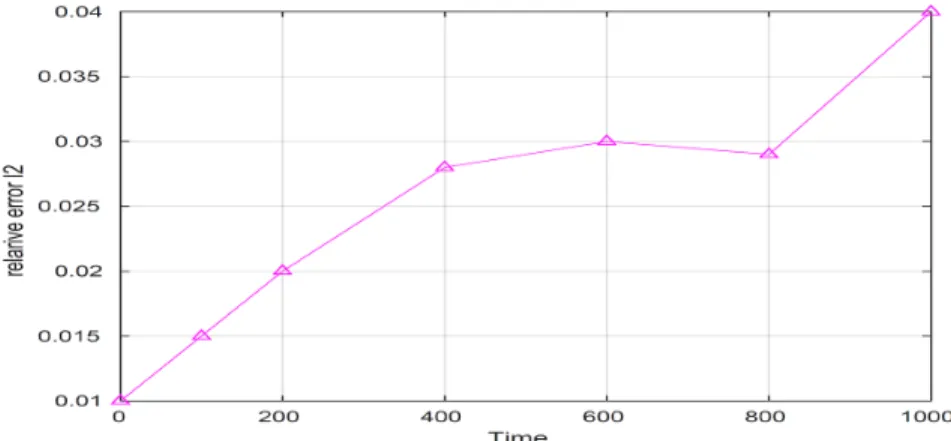
Figure3-3 𝑙2-𝑅𝐸 of free surface elevation for linear SWEs at 𝑡 = 10, 20, ..., 1000 hours. . . . 109
Figure3-4 Comparison 𝑙2-𝑅𝐸 of free surface elevation, 𝑢-velocity and 𝑣-velocity for linear SWEs at 𝑡 = 10, 20, ..., 100 days. . . 109
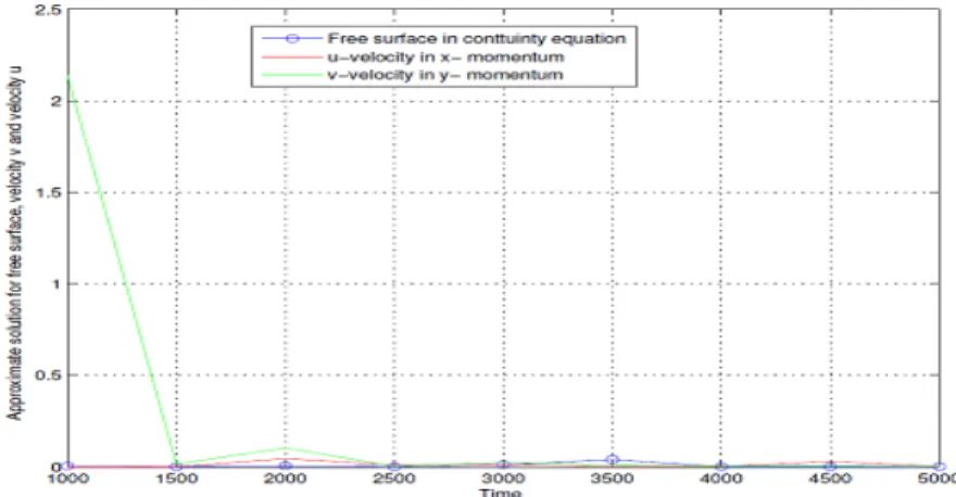
Figure3-5 Comparison the approximate solution for free surface elevation, 𝑢-velocity and 𝑣-velocity for linear SWEs. . . 110
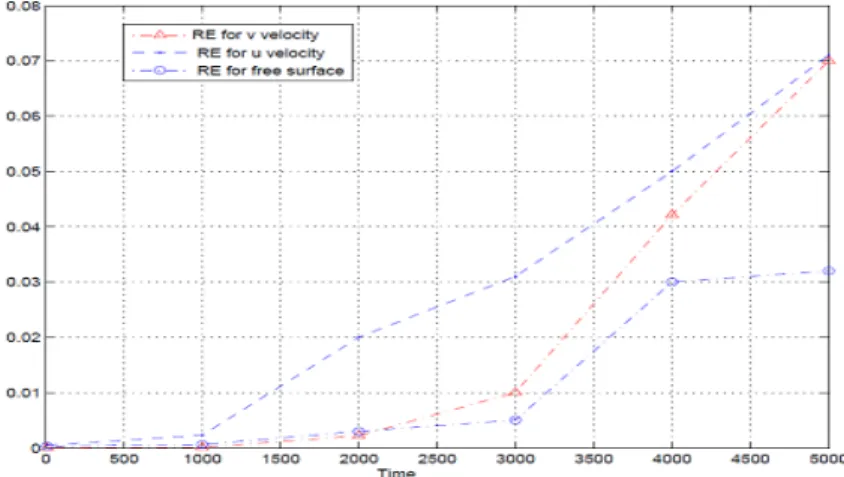
Figure3-6 Comparison 𝑙2-𝑅𝐸 of free surface elevation, 𝑢-velocity and 𝑣-velocity for linear SWEs. . . 111
Figure3-7 Comparison the approximate solution for free surface elevation, 𝑢-velocity and 𝑣-velocity for nonlinear SWEs. . . 111
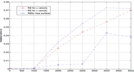
Figure3-8 Comparison 𝑙2-𝑅𝐸 of free surface elevation, 𝑢-velocity and 𝑣-velocity for nonlinear SWEs. . . 112
Figure4-1 Shows Structured grid. . . 124
Figure4-2 Shows unstructured grid. . . 124
Figure4-3 Shows hybrid grid. . . 125
Figure4-5 Overlapping grid configuration. . . 126
Figure4-6 Adaptive mesh refinement. . . 127
Figure4-7 Notations used in the definitions of the nested models. . . 131
Figure4-8 Copy interpolation scheme. . . 133
Figure4-9 Average interpolation scheme. . . 134
Figure4-10 Average interpolation scheme. . . 134
Figure4-11 Shapiro interpolation scheme. . . 135
Figure4-12 Full-weighting interpolation scheme. . . 136
Figure4-13 Full-weighting interpolation scheme. . . 136
Figure4-14 Detailed view of nested grid. Left panel: grid nesting at lower-left corner of sub-level grid region; Right panel: grid nesting at upper-right corner of sub-level grid region. . . 137
Figure4-15 Simulation involving two-way nesting. . . 140
Figure4-16 Simulation involving two-way nesting. . . 142
Figure4-17 Two-way nesting . . . 145
Figure4-18 Embedding the fine grid within the coarse grid. . . 149
Figure4-19 Diagram for open boundary condition. . . 154
Figure4-20 Diagram for two way coupling. . . 155
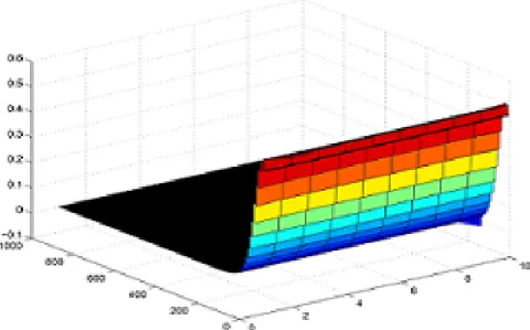
Figure5-1 Simulation of free surface elevation in a coarse grid at time=1000 min. . . 162
Figure5-2 Simulation of free surface elevation in a coarse grid at time=2000 min. . . 163
Figure5-3 Simulation of free surface elevation in a coarse grid at time=3000 min. . . 163
Figure5-4 Simulation of free surface elevation in a finer grid at time=1000 min. . . 164
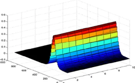
Figure5-5 Simulation of free surface elevation in a finer grid at time=2000 min. . . 164
Figure5-6 Simulation of free surface elevation in a finer grid at time=3000 min. . . 164
Figure5-7 Simulation of free surface elevation in a finer grid at time=2000 hour. . . 165
Figure5-8 Simulation of free surface elevation in two-way nesting grids at time=1000 min. 165 Figure5-9 Simulation of free surface elevation in two-way nesting grids at time=2000 min. 166 Figure5-10 Comparison the approximate solution for free surface elevation between the coarse and the fine grids at 𝑡 = 100 min, 200 min, ..., 2000 min. . . 166
Figure5-11 Simulation of free surface elevation at 𝑡 = 10 min. . . 167
Figure5-12 Simulation of free surface elevation at 𝑡 = 50 min. . . 168
Figure5-13 Simulation of free surface elevation at 𝑡 = 100 min. . . 168
Figure5-14 Simulation of free surface elevation at 𝑡 = 500 hr. . . 168
Figure5-16 Comparison 𝑙2-error norm and 𝐻1-error norm in a coarse grid. . . 169
Figure5-17 Comparison 𝐻1-error norm and 𝑙2-error norm in a fine grid. . . 169
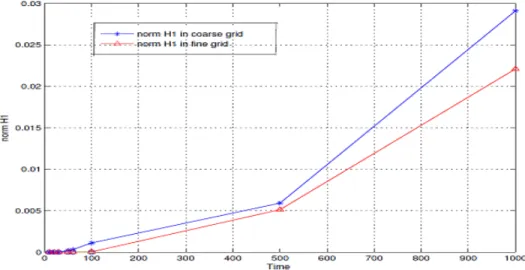
Figure5-18 Comparison 𝐻1-error norm in a coarse grid, and a fine grid for linear SWEs. . 170
Figure5-19 Comparison 𝑙2-error norm in a coarse grid, and a fine grid for linear SWEs. . . 170
Figure5-20 Show 𝑙2-error norm and 𝐻1-error norm in a coarse grid. . . 171
Figure5-21 Comparison 𝑙2-error norm and 𝐻1-error norm in a fine grid at 𝑡=10, 20, ..., 100
days. . . 172
Figure5-22 Show 𝑙2-error norm in a coarse grid, and a fine grid . . . 172
Figure5-23 Show 𝐻1-error norm in a coarse grid, and a fine grid . . . 172
Figure5-24 𝑙2-𝑅𝐸 of free surface elevation between a coarse grid and a fine grid in two-way nested grid. . . 174
Figure5-25 Comparison 𝑙2-𝑅𝐸 between a coarse grid and a fine grid when use four choices of restriction operator for the free surface elevation . . . 174
Figure5-26 Comparison 𝑙2-𝑅𝐸 between a coarse grid and a fine grid when use four choices of restriction operator for free surface elevation . . . 175
Figure5-27 Comparison 𝑙2-𝑅𝐸 between a coarse grid and a fine grid when use four choices of restriction operator for free surface elevation . . . 175
Figure5-28 Comparison 𝑙2-𝑅𝐸 between a coarse grid and a fine grid when use four choices of restriction operator for free surface elevation . . . 176
Figure5-29 Comparison between ABSE and 𝑙2-𝑅𝐸 of free surface elevation in one-way nesting grid when structured grid with a separate interface . . . 177
Figure5-30 Comparison between ABSE and 𝑙2-𝑅𝐸 of free surface elevation in two-way nesting grid when structured grid with a separate interface . . . 177
Figure5-31 Comparison 𝑙2-𝑅𝐸 of free surface elevation in two-way nesting for structured grid with a separate interface . . . 178
Figure6-1 Multiple nested grids at multiple levels . . . 188
Figure6-2 Shows 𝑙2-𝑅𝐸 of free surface elevation between a coarse grid and a in fine grid (grid 21) . . . 189
Figure6-3 Show 𝑙2-𝑅𝐸 of free surface elevation between a coarse grid and a fine grid (grid 22)190 Figure6-4 Comparison 𝑙2-𝑅𝐸 between a coarse grid and two fine grids in level 2 . . . 190
Figure6-5 𝑙2-𝑅𝐸 between the grid 21 and the grid 31 in two-way nested grid . . . 191
Figure6-6 Comparison 𝑙2-𝑅𝐸 between a coarse grid-grid 21 and grid 21-grid 31 . . . 192
Figure6-7 Simulation of free surface elevation in the coarse grid at time= 500 min . . . 193
Figure6-9 Simulation of free surface elevation in the coarse grid at time= 2000 min . . . . 193
Figure6-10 Comparison 𝑙2-𝑅𝐸 of free surface in two-way nested grid at t=500, 1000,..., 4000
hour . . . 194
Figure6-11 Comparison 𝑙2-𝑅𝐸 of free surface elevation between the coarse grid and two fine grids in level 2 . . . 194
Figure6-12 Shows 𝑙2-𝑅𝐸 of free surface elevation between the grid 21 and the grid 31 . . . . 195
Figure6-13 Compares 𝑙2-𝑅𝐸 between a coarse grid-fine grid 22 (level 2) and fine grid 22-fine grid 32 in level 3 . . . 196
Figure6-14 Compares 𝑙2-𝑅𝐸 between a coarse grid-fine grid 21 in level 2 and fine grid 21-fine grid 31 in level 3 . . . 196
Figure6-15 Comparison 𝑙2-𝑅𝐸 between a coarse grid-grid 22 and grid 22-grid 32 for nonlinear SWEs . . . 197
Figure6-16 Comparison 𝑙2-𝑅𝐸 of free surface elevation between a coarse grid-grid 22 for nonlinear case and grid 22-grid 32 for nonlinear to linear . . . 198
Figure6-17 Comparison 𝑙2-𝑅𝐸 between a coarse grid-a fine grid in level 2 for nonlinear to linear and a fine grid in level 2-fine grid in level 3 for linear to nonlinear SWEs . . . . 198
Figure6-18 Comparison 𝑙2-𝑅𝐸 in one-way nesting grid and two-way nesting grid using the average scheme . . . 199
Figure6-19 Comparison 𝑙2-𝑅𝐸 of the free surface elevation in one-way nesting and two-way nesting using Shapiro interpolation scheme . . . 200
Figure6-20 Comparison 𝑙2-𝑅𝐸 in one-way and two-way nesting using the full-weighting scheme . . . 200
Figure6-21 Compares 𝑙2-𝑅𝐸 in two-way nesting using the average scheme and the full-weighting scheme . . . 201
Figure6-22 Compares 𝑙2-𝑅𝐸 in two-way nesting using the average scheme and the full-weighting scheme . . . 201
Figure6-23 ABSE and 𝑙2-𝑅𝐸 of free surface elevation in one-way nesting . . . 202
Figure6-24 ABSE and 𝑙2-𝑅𝐸 of free surface elevation in two-way nesting . . . 203
Figure6-25 ABSE between the coarse grid and the fine grid for linear 2DSWEs . . . 203
Figure6-26 Comparison 𝑙2-𝑅𝐸 and ABSE in two-way nesting grids . . . 204
Figure6-27 𝑙2-𝑅𝐸 of free surface elevation in one-way nesting grid for linear SWEs . . . 205
Figure6-28 𝑙2-𝑅𝐸 of free surface elevation in two-way nesting grid for linear SWEs . . . 205
Figure6-29 𝑙2-𝑅𝐸 of free surface elevation in one-way nesting grid for nonlinear SWEs . . . 205
Figure6-31 𝑙2-𝑅𝐸 in two-way nesting using four different update schemes without separate
dynamic interface and feedback interface . . . 207
Figure6-32 𝑙2-𝑅𝐸 in two-way nesting using four different update schemes with separate dy-namic interface and feedback interface . . . 207
Figure6-33 Free surface elevation on the coarse grid domain using average method. . . 208
Figure6-34 Free surface elevation on the coarse grid domain using mix-low method . . . 209
Figure6-35 Free surface elevation on the coarse grid domain using full-weighting method . . 210
Figure6-36 Free surface elevation on the coarse grid domain using mix-high method . . . 211
Figure6-37 Comparison the ABSE between a coarse grid and a fine grid in level 2 . . . 212
Figure6-38 Comparison the ABSE between level 2 and level 3 . . . 212
Figure6-39 Comparison 𝑙2-𝑅𝐸 between a coarse grid-a fine grid (level 2) and level 2-level 3 213 Figure6-40 Comparison 𝑙2-𝑅𝐸 when use four choice for update schemes with a separate interface213 Figure6-41 Comparison 𝑙2-𝑅𝐸 when use four choice for update schemes without a separate interface . . . 214
Figure7-1 Comparison 𝑙2-𝑅𝐸 between a coarse grid- fine grid in level 2 and level 2-level 3 in case space refinement ratio is 1:5 . . . 221
Figure7-2 Comparison 𝑙2-𝑅𝐸 between a coarse grid in level 1-fine grid in level 2 and fine grid in level 2-fine grid in level 3 in case the space refinement ratio is 1:3 . . . 221
Figure7-3 Comparison 𝑙2-𝑅𝐸 between a coarse grid in level 1-fine grid in level 2 and fine grid in level 2-fine grid in level 3 in case 1:5 . . . 222
Figure7-4 Comparison 𝑙2-𝑅𝐸 between a coarse grid in level 1-fine grid in level 2 and fine grid in level 2-fine grid in level 3 in case 1:3 . . . 222
Figure7-5 Comparison 𝑙2-𝑅𝐸 and ABSE in one-way nesting in case 1:4 . . . 223
Figure7-6 Comparison 𝑙2-𝑅𝐸 and ABSE in two-way nesting in case 1:5 . . . 223
Figure7-7 Comparison ABSE between a coarse grid in level 1-fine grid in level 2 and fine grid in level 2-fine grid in level 3 . . . 224
Figure7-8 Comparison 𝑙2-𝑅𝐸 between a coarse grid in level 1-fine grid in level 2 and fine grid in level 2-fine grid in level 3 for 2DNSWEs . . . 225
Figure7-9 Comparison 𝑙2-𝑅𝐸 and ABSE for one-way nesting in case 1:3 . . . 225
Figure7-10 Comparison 𝑙2-𝑅𝐸 and ABSE for two-way nesting in case 1:3 . . . 226
Figure7-11 Comparison 𝑙2-𝑅𝐸 and ABSE for one-way nesting in case 1:4 . . . 226
Figure7-12 Comparison 𝑙2-𝑅𝐸 and ABSE for two-way nesting in case 1:5 . . . 226
Figure7-13 Comparison 𝑙2-𝑅𝐸 of free surface elevation , 𝑢-velocity and 𝑣-velocity . . . 227
Figure8-2 Comparison 𝑙2-𝑅𝐸 of free surface between a coarse grid and level 2 (grid 21 and grid 24) . . . 238 Figure8-3 Comparison 𝑙2-𝑅𝐸 between a coarse grid and level 2 (grid 22 and grid 23) . . . 238 Figure8-4 Comparison 𝑙2-𝑅𝐸 between coarse grid-level 2 (grid 21), level 2-level 3 (grid 32)
and level 3-level 4 (grid 43) . . . 239 Figure8-5 Comparison 𝑙2-𝑅𝐸 between a coarse grid-level 2 (grid 24), level 2-level 3 (grid
33), and level 3-level 4 (grid 46) . . . 240 Figure8-6 Comparison 𝑙2-𝑅𝐸 of free surface elevation between a coarse grid-level 2 (grid
23), level 2-level 3 (grid 34) and level 3-level 4 (grid 44) . . . 241 Figure8-7 Comparison 𝑙2-𝑅𝐸 between a coarse grid-level 2 (grid 23) and level 2-level 3 (grid
34) and level 3-level 4 (grid 42) . . . 242 Figure8-8 Multiple nested grids at multiple levels for linear 2DSWEs . . . 242 Figure8-9 Show 𝑙2-𝑅𝐸 between a coarse grid and four fine grids (21, 22, 23 and 24) . . . . 243 Figure8-10 Comparison 𝑙2-𝑅𝐸 of free surface elevation between a coarse grid-level 2 (grid
21), level 2-level 3 (grid 32) and level 3-level 4 (grid 43) . . . 244 Figure8-11 Comparison 𝑙2-𝑅𝐸 between a coarse grid-level 2 (grid 22), level 2-level 3 (grid
33) and level 3-level 4 (grid 44) . . . 245 Figure8-12 Comparison 𝑙2-𝑅𝐸 between a fine grid in level 2 and level 3 (grid 32) in cases
separate and embedded grids. . . 246 Figure8-13 Comparison 𝑙2-𝑅𝐸 for linear 2DSWEs when time step 0.010 . . . 247 Figure8-14 Comparison 𝑙2-𝑅𝐸 for linear 2DSWEs when time step 0.030 . . . 247 Figure8-15 Comparison 𝑙2-𝑅𝐸 between a coarse grid-level 2 (grid 24), level 2-level 3 (grid
31) and level 3-level 4 (grids 41) . . . 248 Figure8-16 Comparison 𝑙2-𝑅𝐸 of free surface elevation between a coarse grid-level 2 (grid
24), level 2-level 3 (grid 31) and level 3-level 4 (grids 45)embedded with itself . . . 249 Figure8-17 Comparison 𝑙2-𝑅𝐸 between level 1-level 2, level 2-level 3 and level 3-level 4 . . 250 Figure8-18 Comparison 𝑙2-𝑅𝐸 between level 1-level 2 in case nonlinear, level 2-level 3 in case
nonlinear to linear and level 3-level 4 in case linear to nonlinear SWEs. . . 250 Figure8-19 Comparison 𝑙2-𝑅𝐸 between a coarse grid-fine grid in level 2 nonlinear to linear
case, fine grid in level 2-fine grid in level 3 linear to nonlinear case and level 3-fine grid in level 4 nonlinear to linear case. . . 251 FigureA-1 A sketch of moving boundary scheme . . . 268
List of Tables
Table4.1 Shows the restriction operator for free surface elevation 𝜂 and velocities (𝑢, 𝑣) on Arakawa C-grid. . . 151 Table6.1 The information on the set up of the different grids for 2D non-linear SWEs . . 189 Table6.2 The information about the coarse and fine grids for linear 2DSWEs . . . 190 Table6.3 The information about the coarse and the fine grids at multiple levels for linear
2DSWEs . . . 191 Table6.4 The information about the coarse and the fine grids at multiple levels for 2DNSWEs
. . . 195 Table6.5 The information about the coarse grid and the fine grids at multiple levels for the
2DNSWEs . . . 197 Table7.1 The information about the coarse and fine grids at multiple regions (levels) for
2DNSWEs . . . 220 Table8.1 The information on the set up of the different grids . . . 237 Table8.2 The information on the set up of the different grids for 2DNSWEs . . . 239 Table8.3 The information on the set up of the different grids at multiple level for 2DNSWEs 240 Table8.4 The information on the set up of the different grids at multiple levels . . . 241 Table8.5 The information on the set up of the different grids at multiple levels for linear
SWEs . . . 243 Table8.6 The information on the set up of the different grids at multiple levels for linear
2DSWEs . . . 244 Table8.7 The information on the set up of the different grids at multiple levels for linear
SWEs . . . 245 Table8.8 The information on the set up of different grids for linear SWEs . . . 246 Table8.9 The information on the set up of the different grids at multiple levels for linear
2DSWEs . . . 247 Table8.10 The information on the set up of the different grids at multiple levels . . . 248 Table8.11 The information on the set up of the different grids at multiple levels for 2DNSWEs 249
Outline of This Work
The major purpose of our work is to design new technique for multiple nested grids of 2D non-linear shallow water equations (2DNSWEs) for structured grids using numerical schemes.
This thesis is organized into four parts with 9 chapters. The general framework of the various topics will be detailed in the parts and chapters that follow:
Part I: Mathematical and Numerical Model for 2D Depth-Integrated Shallow Water Equations
The principal objective of this part is to study the development of the efficiency of numerical methods for 2D depth-averaged non-linear shallow water models by proposing new spatial and temporal discretization techniques in a standard C-grid using an explicit finite difference method in space and leapfrog with Robert-Asselin filter in time. Firstly, a new technique to derive 2DSWEs is presented. Secondly, propose effective numerical methods, such as the explicit finite difference methods for solving ocean models. The different unknowns variables for the system are approximated on staggered grids and the numerical fluxes are computed with the proposed techniques.
This part consists of three chapters including:
Chapter 1: Derivation of 2D Shallow Water Equations
This chapter is devoted to the study of 2D non-linear shallow water equations. Firstly, presents a mathematical study of Navier-Stokes equations and 2DSWEs, which are obtained from a vertical integration of 3D Navier-Stokes equations by using a number of the assumptions. Secondly, we know that 2DSWEs can be derived in a number of ways with varying initial assumptions, we suggest two ways to expand the derivation of 2D depth-averaged SWEs from 3D Navier-Stokes equations using splitting of velocity and eddy dispersion coefficients. Another way is presented to derive 2DSWEs without using depth-averaged technique.
Chapter 2: An Explicit Staggered Finite Difference Scheme for 2D Shallow Water Equa-tions (Numerical Techniques for 2DSWEs)
This chapter is a description of the development and evaluation of proposed numerical methods for 2D shallow water models, which depend on the choice of techniques and numerical methods used.
Chapter 3: Numerical Results for 2D Shallow Water Equations (Validations of the Model).
In order to validate the proposed method of 2D shallow water equations, some examples of the tsunami model are applied. Some examples for 2DSWEs are tested using Gaussian level initial con-dition. The application for rotating or (non-rotating) shallow water equations are given. Full model of 2DSWEs including Coriolis force as the source terms are considered. The numerical simulations are implemented by computer programming using Matlab and Fortran 90 under Dirichlet, reflexive boundary conditions and moving boundary conditions.
Part II: Coupling for Two-Way Nesting Grids: Mathematical Framework and Appli-cations for Shallow Water Model (Nested Grid For 2D Shallow Water Equations)
In the major part of the thesis, we are interested to propose a new two-way interaction technique for multiple nesting grids to solve ocean models. This part consists of two chapters:
Chapter 4: The Configuration a Nested Grid for Shallow Water Models
A literature review of techniques used to try to increase the efficiency and accuracy of 2D shallow water models are presented. Some new algorithms are established to implement two-way interaction technique for this model. Two-way nesting systems depend on the type of interpolation, the location of the dynamical interface, conservation properties and type of update. Different cases of open boundary conditions for two-way nesting grids are studied.
In this chapter, looks into the optimum feedback conditions and interpolation techniques to maximize the feedback of the information and to ensure the conservation of properties. Four choices of the update scheme for the free surface elevation and velocities on Arakawa C-grid are applied.
Chapter 5: Performance of Two-Way Nesting Techniques for Shallow Water Equations The principal objective of this chapter is to study the accuracy of two-way nesting performance techniques for structured grids between a coarse grid and a fine grid for 2DSWEs using an explicit finite difference methods with the refinement ratio 1:3.
We present and evaluate a set of options that made implementation of two-way nesting methods allowing simultaneous spatial and temporal refinement in shallow water model. Results showed two-way nested model can produce accurate high-resolution solutions in areas of interest and improve the realism of the solution in the low-resolution coarse domain for a much lower computational effort than the standard single grid high-resolution model.
Part III: Implementation and Validation of Solutions For 2D Shallow Water Models: This part includes
Chapter 6: Applications of Two-way Nesting Technique for Multiple Nested Grids with Nesting 3:1 at Multiple Levels
Multiple nested grids can be employed together to save the time as well as obtain enough resolution in the goal region. In this chapter, the explicit finite difference methods which are used to construct a two-way nesting technique are applied successfully for a multiple-nested grid 2DNSWEs for structured grids when the refinement ratio is 1:3 using new algorithms and techniques provided underChapter 4. In order to verify the performance of nesting technique, apply some examples of coupling 3 systems for shallow flow models. Comparison of 𝑙2-relative error norm (𝑙2-𝑅𝐸) results for one-way and two-way nesting grids using four update interpolations. Finally, comparison of 𝑙2-relative error norm (𝑙2-𝑅𝐸) results to the free surface elevation for some examples using four options of restriction operator with two cases of the refinement ratio.
Chapter 7: Multiple Nested Model for 2D Non-Linear Shallow water Equations with Nesting 5:1 at Multiple Levels
A two-way interaction technique for multiple nested grids of 2D non-linear shallow water models is constructed and it is applied when the refinement ratio 1:5.
Part IV : Numerical Results of The Tsunami Model
In this part, we discuss some numerical results of the tsunami model.
Chapter 8: Some Applications for Multiple Nested Grids of the Tsunami Model
Several examples for multiple nested grids of the tsunami model are applied when space refinement ratio is 1:5 and the temporal refinement ratio is 1:2 for 2D non-linear SWEs. The performance and accuracy of the model are tested and the results show are good.
Chapter 9: Some Recommendations (Future Works)
Some possible recommendations for future methods of research progress are presented.
All the numerical simulations are performed by computer programming using Matlab and Fortran 90.
Some Publications
This thesis contains several chapters including some articles which are published or sub-mitted:
1. Some Sections in Chapters 1 and 2: It has been published in proceeding as: Huda Altaie, New Techniques of Derivations for 2D Shallow Water Equations, International Journal of Advanced Scientific and Technical Research, Issue 6 volume 3, May-June 2016.
2. Chapter 3: It has been published in proceeding as: Huda Altaie and Pierre Dreyfuss, Numerical Solutions For 2D Depth-Averaged Shallow Water Equations, International Mathematical Forum, Vol.13, 2018, no.2, 79-90.
3. Some Sections in Chapters 4 and 5: It has been published in proceeding as: Huda Altaie, A Two-Way Nesting for Shallow Water Model, International Review of Physics (I.RE.PHY.), Vol. 11, N. 4, ISSN 1971-680X, August 2017.
4. Some Sections in Chapter 6: It has been submitted as: Huda Altaie and Fabrice Planchon, Results of higher accuracy for 2D shallow water equations with (separate/adjacent) for structured grids, 2018.
5. Some Sections in Chapter 6: It has been published in proceeding as: Huda Altaie, A Multiply Nested Model for Non-Linear Shallow Water Model, Journal of Research and Reports on Mathematics, Vol 1, no.2, 2018.
6. Chapter 7: It has been published in proceeding as: Huda Altaie, Numerical Model for Nested Shallow Water equations, International Journal of Pure and Applied Mathematics- IJ-PAM, Vol 118, no.4, 1033-1051, 2018.
7. Chapter 8: It has been published in proceeding as: Huda Altaie, Application of a Two-Way Nested Model for Shallow Water, Journal of Research and Reports on Mathematics, 2018.
Other Publications
1. Huda Altaie,Numerical Methods for Solving the First order linear Fredholm-Voltterra integro Differential Equations, Journal of Al Nahrain University Vol.12 (2), June, pp.123-127, 2009.
2. Huda Altaie, Numerical Methods for Solving Linear Fredholm-Voltera integral equa-tions, Journal of Al Nahrain University Vol.11(3), December, pp. 131-134, 2009.
3. Huda Altaie, Modified Third Order Iterative Method for Solving Nonlinear Equations, Journal of Al Nahrain University Vol.16 (3), September, 2013, pp.239 -245.
4. Huda Altaie, Modified Mid-Point method Method For Solving Linear Fredholm In-tegral Equations Of The Second Kind, Journal of Al-Qadisiyah for Computer Science and Mathematics Vol.3 No.1, 2011.
5. Huda Altaie, Solutions of Systems for the Linear Fredholm-Voltterra Integral Equa-tions of the Second Kind, Ibn Alhaitham J. Vol.23 (2) 2010.
6. Huda Altaie, Solutions for linear Fredholm-Voltterra integral Equations of The second Kinds using the Repeated Corrected Trapezoidal and Simpson Methods, Journal of Al Nahrain University Vol.13(2), june 2010, pp.194 -204.
7. Huda Altaie, Easy Numerical Method to Solution a System of Linear Voltterra Integral Equations, Journal of Al Nahrain University Vol.14, September pp.144-149, 2011.
Mathematics Notations
𝐶 Chezy bed roughness coefficient or Ekman coefficient 0.026.
𝐶𝐷 The dimensionless coefficient of quadratic friction. Here, the quadratic drag coefficient
is taken usually 𝐶𝐷 = 2.5.10−3 but it may also take into account the bottom roughness.
c Coarse grid/ parent grid.
𝐶𝑎 Air drag coefficient, is taken usually 𝐶𝑎= (0.8 + 0.0658
√
𝑢10+ 𝑣10) × 10−3
where 𝑢10 and 𝑣10 shown below.
𝐶𝑛 Courant number.
𝑓 Coriolis parameter, f= 2𝜔𝑠𝑖𝑛𝜑 , where 𝜔 is the earth’s angular velocity (𝑠−1)and
𝜑 is north latitude (positive northward), 𝑓 = 1.01 × 10⁻⁴ Coriolis frequency at 42 latitude.
𝐹 Volume force.
𝑔 Acceleration due to gravity (𝑔 = 9.81𝑚𝑠−2).
𝐻 Total depth (h+𝜂), where h is the mean sea depth (m) (or sometimes called water depth). − → ▽ Gradient operator −→▽ = (𝜕 𝜕𝑥, 𝜕 𝜕𝑦, 𝜕 𝜕𝑧). △ Laplacien operator −→▽2= (𝜕 𝜕𝑥( 𝜕 𝜕𝑥), 𝜕 𝜕𝑦( 𝜕 𝜕𝑦), 𝜕 𝜕𝑧( 𝜕 𝜕𝑧)). Ω Domain of calculation
𝑡, △𝑡, △𝑥, △𝑦 Time (s), time step, 𝑥-direction grid spacing, and 𝑦-direction grid spacing respectively. (𝑥, 𝑦) Horizontal Cartesian spatial coordinates (𝑚)
𝜂 Elevation of the sea surface above mean sea level (or high surface water, free surface elevation). (𝑢, 𝑣) Components of velocity in the 𝑥 and 𝑦-directions respectively
𝑢10, 𝑣10 The vertically averaged air velocities at a distance of 10𝑚 above the sea surface (𝑚𝑠−1).
q Vector velocity field (𝑚𝑠−1).
𝜌 Density of the fluid (sea water) assumed constant (= 1027𝑘𝑔𝑚−3). 𝜌𝑎 Density of air assumed uniform (water density) (= 1.225𝑘𝑔𝑚−3).
𝜌0 Water mean density (= 1.033𝑘𝑔𝑚−3).
𝜈 Coefficient of viscosity (𝑚𝑠−2).
𝑝, 𝑝𝑎 The pressure, and pressure at the surface respectively.
𝜏𝑖,𝑗 Viscous shear stress in 𝑖-direction on a 𝑗-plane.
(𝑢, 𝑣) Components of depth-averaged velocity (mean) in the 𝑥 and 𝑦-directions respectively ̃︀
𝑢 The deviation of the mean velocity. ̃︀
𝑢𝑖 𝑢̃︀𝑗 Reynold stress.
𝜔 = 86164𝑠2𝜋 Angular velocity due to rotation of the earth.
Glossary
Shallow water equations SWEs
2D Shallow water equations 2DSWEs
Nonlinear Shallow water equations NSWEs
𝑙2-relative error norm 𝑙2-𝑅𝐸
3D Navier-Stokes equations 3DNSEs
Explicit finite difference method EFDM
Absolute error ABSE
Partial Differential Equations PDEs
Development of 2DSWEs (Goals and Objectives)
The development of the efficiency and advantage of numerical methods for shallow water models are carried out in the following stages:
1. Propose a new technique for deriving 2DSWEs using splitting of velocity and horizontal eddy viscosity.
2. Suggest some ways to expand the derivation of 2D depth-averaged SWEs using 3D Navier-Stokes equations. Another way is presented to derive 2DSWEs without using depth-averaged technique. 3. New spatial and temporal discretization techniques in a standard C-grid using an explicit finite
difference method and leapfrog with Robert-Asselin filter for 2DSWEs are applied.
4. Investigation of the proposed techniques which are able to solve 2DSWEs and some examples of the tsunami mode under moving boundary conditions are tested.
5. Dynamical coupling in a two-way nesting system is performed at a dynamical interface which is a separate/adjacent from a mesh interface.
6. Build some new algorithms to implement two-way interaction technique for ocean models. 7. Four choices of restriction operator for the free surface elevation and velocities on Arakawa
C-grid are applied. The choice of the full-weighting and the average update operators are proposed which have the excellent properties regarding the filtering.
8. Suggested a new technique for multiple nested grids at multiple levels for shallow water models with nest 3:1 and 5:1.
9. Coupling multi systems for multiple nested grids are achieved for 2DSWEs with nest 3:1 and 5:1 at multiple levels.
10. Apply the proposed technique to multiple nested grids for some examples of the tsunami model. 11. All the simulation are made by using Dirichlet condition, reflexive conditions and moving bound-ary conditions. Boundbound-ary conditions for the nested domain are linearly interpolated from the coarse domain and feedback using the average scheme or (full-weighting scheme) with (sepa-rate/adjacent) dynamic interface and feedback interface from the high-resolution nested grids solution to the low-resolution coarse grids solution.
General Introduction
Background and Review
For oceanic phenomena problems such that complex geometry (i.e., with rivers and estuaries), in order to increase the horizontal resolution in a subregion without incurring the computational expense of high resolution over the entire domain. One effective way to overcome this difficulty is to build hierarchies of nested models with a focus on the area of interest. This technique has been widely used in meteorology and in oceanography, for which some examples of applications can be found in[90, 109]. The success or failure of these efforts will depend both on the nesting technique and on the charac-teristics of the basic ocean model. Conclusions on how nested models perform may depend on options of test problems. There are great works of literature describing nested models for the ocean. Major efforts include ([16, 36, 56, 90, 102, 109]). The drawback of this technique is the great number of pa-rameters or the generation of new problems grid interaction, computational efficiency, and conservation properties (flux of mass and momentum) compared with a classical technique with a single expandable grid.
This system allows a local increase of the mesh resolution in areas where it seems to be necessary, by running the same model on a hierarchy of grid. Nesting (or embedding) techniques for structured mesh generally which indicate an economical way to improve the horizontal resolution, consists a local high-resolution grid embedded in a coarser-resolution one which covers the entire domain. In the case of one-way interaction, coarse grid solution provides boundary conditions for the high-resolution grid. In two-way nesting, the fine grid results are feedback to the coarse grid in addition to the use of the coarse grid results in specifying the boundary conditions of the fine grid. The interaction between the coarse grid and fine grid in two-way nesting can take place either at the dynamic interface between them [122] or over their overlapping region [90]. These methods have been applied successfully in atmosphere and ocean modelling ([36, 48, 52, 53, 99, 104]).
The nesting procedure should preferably conserve fluxes of mass and momentum across the inter-faces. In meteorology, such a scheme was developed by Kurihara et al. [122]. Berger[13]have developed general adaptive mesh refinement algorithms for hyperbolic systems that also are conservative across interfaces. Ginis et al. [102] applying the technique proposed by Kurihara et al. [122] developed a nested primitive equation model that did not fictitiously increase or decrease the transports of mass, momentum, and heat through the dynamical interface. Angot[94] address the continuity and conser-vation properties across interfaces. Rowley and Ginis [27] included a mesh movement scheme in the
nested ocean model and stated that mass, heat, and momentum are conserved during the movement. Most papers describing nested ocean modelling efforts discuss stability problems and unsmooth solutions across the interfaces. Spall [109] finding support in Zhang [52] state that it may be neces-sary to sacrifice exact conservation to obtain smooth, stable solutions. To stabilize, and smooth the solutions we find that combinations of horizontal and vertical diffusion, altering the solutions in time and relaxation techniques or nudging are often applied.
In the literature, both one-way and two-way interaction between the coarse and the fine grid have been considered. In the case of one-way interaction, coarse grid solution supply boundary conditions for the fine grid, but there is no feedback from the fine grid. Phillips and Shukla [98] argue that a way interaction gives correct solution on the fine grid and therefore is more favorable. The two-way nesting described in [90, 102, 109]. Also, a recent survey of two-way embedding algorithms can be found in ([16, 19, 47, 66]).
The various two-way interaction schemes mainly differ by type of interpolation, the location of dynamical interface, conservation properties (flux of mass, and momentum equations), and type of update.
However, a two-way interaction may introduce instabilities at the interface between the two grids, and such instabilities may lead to a severe degradation solution [52]. In some studies data from previously run coarse grid models are used to drive fine grid models ([65, 111]). Fox [56] compared one-way and two-way nesting and concluded that using the model in one-way nesting mode resulted in more noise at the fine grid mesh boundaries with a negligible decrease in computer time. In order to provide the boundary condition for the fine grid, the coarse grid variables must be interpolated to the fine grid. There are numerous techniques that are potentially interesting for performing two-way nesting (see [83, 102]). Based on studies with an idealized test case, they conclude that zeroth-order interpolation may create large phase errors, quadratic interpolation may create overshooting and they suggest the use of advection equivalent interpolation schemes.
Nested model grids may be adaptive and movable or static. In order to follow evolving oceanic features such as wavefronts and propagating eddies it may be beneficial to apply for instance adaptive mesh refinement methods for hyperbolic systems described by[13]or more recently by[16, 19, 47, 66]
have recently applied this technique to study the propagation of the barotropic model and with a multi-layered quasi-geostrophic model.
Spall and Holland[109]apply the same time step both on the coarse and the fine grid arguing that the coarse grid contributes little to the overall expense and that it would add an additional level of computational complexity for very little gain to have different time steps on the two grid levels. With equal Courant numbers on all levels the quality of the wave propagation relative to the mesh size will be approximately the same, and most of the more papers on nesting also refine the time step with the
same factor as the spatial resolution, keeping the Courant numbers constant.
Warner et al[97]recommend using two-way nesting whenever possible since the solution is presumed to be more accurate when the coarse and nested grid solutions are allowed to interact with one another. Phillips[98] studied the distortion of shallow-water Rossby and gravity waves in simulations using both a one-way and a two-way nest. The authors claimed that the two-way solution is more accurate than the one-way solution because coarse grid solution is nearer to that on the nested grid but they do not elaborate on this rather obvious point. In particular, there is no analysis of why reflections may be less when using two-way nesting.
Clark[25]and Chen[24]both performed simulations of two-dimensional linear vertically propagat-ing mountain waves uspropagat-ing nested grids to increase both the horizontal and vertical resolution near the mountain and they did not use the interpolation boundary condition but instead linearly interpolated fluxes to the boundary of the nested grid. This approach yields conservation of mass and momentum across the nested grid boundary which is a desirable property for some modelers.
Chen [24] used a similar nesting strategy in a fully compressible model to test several different boundary conditions including the interpolation boundary condition and a continuously stratified vari-ant of the inflow-outflow boundary condition for shallow water flow[20].
In ocean model, the nesting is the degree of refinement from one level to the next and the grid ratio from 2:1 to 7:1 has been applied. Spall and Holland [109] conclude that 3:1 and 5:1 ratios perform quite well, and even ratio of 7:1 are able to reproduce the solution reasonably well while the features are mostly contained within the fine region. To apply small ratios like 2:1, which is used for instance in Rowley and Ginis [27], may force us to apply many grid levels before we achieve the resolution we would like to have in a given area. On the other hand, large ratios may cause instabilities and non-smooth solutions across the interfaces. There are numerous combinations of basic ocean models and nesting techniques that are potentially interesting and evidence on how these groups perform is gradually growing as they are applied both to idealized test cases and for more realistic oceanic problems[73, 90, 94].
Part I
Mathematical and Numerical Model For 2D
Depth-Averaged Shallow Water Equations
Chapter 1
Chapter 1
Derivation of 2D Shallow Water Equations
The results presented in this chapter (Sections 1.4 and 1.5) are the subject of the article [2].
As we know, there are several possible strategies to derive 2D non-linear shallow water equations. The first possibility is to integrate the 3D Navier-Stokes equations over the vertical direction and take averaged values for the velocities. The second alternative is to consider conservation laws for mass and momentum directly on an infinitesimal control volume.
This chapter focuses on the derivation of 2D depth-averaged SWEs in a manner that hopes to highlight the important assumptions required. Several approaches can be used to develop this deriva-tion, we suggest two ways to expand the derivation of 2D shallow water flow from 3D Navier-Stokes equations using splitting of velocity and horizontal eddy viscosity. Another way is introduced to derive this model without using the depth-averaged technique.
Highlights
∙ Mathematical description of 3D Navier-Stokes equations is presented. ∙ The complete derivation of 2DSWEs is explained .
1.1 Introduction
Shallow water equations are hyperbolic partial differential equations (or parabolic if viscous shear is considered) which explain the flow behavior of rivers. These equations were established in (1775) by Laplace and were first used in (1871) by the physicist Adhémar Jean Claude Barré de Saint-Venant. More generally, SWEs describe the evolution of unsteady flow (incompressible) of a fluid, not necessarily water with constant density. This system is essentially based on the assumption that the water depth is shallow.
This assumption implies that the model is hydrostatic and state that the velocity is constant with the depth, bounded from below by the bottom topography and from above by the water surface. The 3D incompressible Navier-Stokes equations are averaged over the depth to obtain SWEs.
These equations are applicable to mathematical concepts where the typical vertical scale is neg-ligible compared to the typical horizontal scale, and they are effective for many physical phenom-ena in the oceans, coastal regions, rivers and canals, lake hydrodynamics, dam breaks,...etc (see
[30, 40, 57, 73, 85, 87, 95, 101]).
The derivation of shallow water models effects has received an extensive coverage [63, 105] and numerical techniques for the approximation of these models have been recently proposed[33, 72]. This technique for deriving of non-linear SWEs is classical when the viscosity or the wind effects on the free surface are neglected [45, 54]. In the literature, we often find various non-linear SWEs which may include wind effects on the free surface, bottom topography and friction effects on the bottom, often defined using the Manning Chezy formula, or viscosity[43, 45, 68]. Several variations for shallow water models can be constructed from different assumptions regarding the nature of the fluid, such as viscosity, incompressibility, and properties of the domain in which the fluid is situated.
This chapter is devoted to highlighting some essential properties of 2DSWEs; it is organized as follows: Derivation of 2DSWEs is described so that they can be derived in a number of ways with varying initial assumptions and mathematical complexity. In Sections 1.2 and 1.3, we recall the mathematical description of 3D Navier-Stokes equations and 2DSWEs. A new technique for complete derivation for 2D non-linear SWEs is constructed in Sections1.4 and 1.5. Finally, another way without using depth-averaged technique to derive this model is introduced in Section 1.6.
Figure 1-1: Shallow water equations in canals.
Figure 1-2: Shallow water equations in dam break.
1.2 Mathematical Description for 3D Navier-Stokes Equations
The Navier-Stokes equations are based on Newton’s second law and consist of a time-dependent con-tinuity equation for conservation of mass, three time-dependent conservation of momentum equations which actually results from the fundamental relationship of fluid dynamics. These equations describe how the velocity, pressure, temperature, and density of a moving fluid are related. The equations were derived independently by G.G. Stokes, in England, and M. Navier, in France, in the early 1800’s, which are obtained from the two basic principles of physical laws: ([71, 117]).
1.2.1 The conservation of mass law
The conservation of mass is the first principle used to develop the basic equations of fluid mechanics. Simply the conservation of mass implies that the total mass of a closed system in a region Ω is constant over time and mass can neither be created nor destroyed, where Ω ∈ 𝑅3 (see[51, 118]).
The general formula of the mass continuity in conservation form is: 𝜕𝜌 𝜕𝑡 + 𝜌 (︂ 𝜕𝑢 𝜕𝑥+ 𝜕𝑣 𝜕𝑦 + 𝜕𝑤 𝜕𝑧 )︂ = 0
If the fluid density is constant, the physical interpretation of the equations implies that the change of density of a fluid particle is equal to the expansion of the fluid. Also, when assuming the fluid is incompressible. This means that 𝜌 does not depend on 𝑝 (𝜌=𝜌0 is constant), which is not a necessary
condition for incompressible flow, thus the derivative of the density over time is zero. (︂ 𝜕𝑢 𝜕𝑥 + 𝜕𝑣 𝜕𝑦 + 𝜕𝑤 𝜕𝑧 )︂ = 0
1.2.2 The conservation of momentum
The conservation of momentum rule is based on Newton’s second law which states that: if the resulting force 𝐹 acts on a body of mass 𝑚, then the rate of increase of linear momentum is equal to the force 𝐹 (see [51, 118]). For an incompressible fluid and constant viscosity, the mathematical equation representing this law is:
𝐷𝑞 𝐷𝑡 = −
1
𝜌. ▽ 𝑝 + 𝜈 ▽
2(𝑞) + 𝐹
Physical meaning of each term (a) 𝐷𝑞
𝐷𝑡 Change in velocities over time, where 𝐷/𝐷𝑡 is the material or total derivative.
(b) ▽𝑝 The internal pressure gradient of the fluid (the change in pressure) (c) 𝜈 ▽2(𝑞) The internal stress forces acting on the fluid.
(d) 𝐹 The external stress forces acting on the fluid.
1.2.3 Stress components
The stress state is represented as a symmetric tensor 𝜏, whose components may be expanded in to various coordinate systems. The components of the velocity vector (𝑢, 𝑣, 𝑤) align with the Cartesian-Coordinate directions (𝑥, 𝑦, 𝑧). For such fluids are called Newtonian fluids. If assume an incompressible fluid the components of stress tensors as follows: [91, 118].
𝜏𝑥𝑥 = 𝜇. (︂ 𝜕𝑢 𝜕𝑥 + 𝜕𝑢 𝜕𝑥 )︂ , 𝜏𝑦𝑦= 𝜇. (︂ 𝜕𝑣 𝜕𝑦+ 𝜕𝑣 𝜕𝑦 )︂ , 𝜏𝑧𝑧 = 𝜇. (︂ 𝜕𝑤 𝜕𝑧 + 𝜕𝑤 𝜕𝑧 )︂ 𝜏𝑥𝑦 = 𝜏𝑦𝑥= 𝜇 (︂ 𝜕𝑢 𝜕𝑦 + 𝜕𝑣 𝜕𝑥 )︂ , 𝜏𝑥𝑧 = 𝜏𝑧𝑥= 𝜇 (︂ 𝜕𝑢 𝜕𝑧 + 𝜕𝑤 𝜕𝑥 )︂ , 𝜏𝑦𝑧 = 𝜏𝑧𝑦 = 𝜇 (︂ 𝜕𝑤 𝜕𝑦 + 𝜕𝑣 𝜕𝑧 )︂
where 𝜇 is called the coefficient of dynamic viscosity and the kinematic viscosity 𝜈 = 𝜇 𝜌.
In general, 𝜏𝑖,𝑗represent the viscous shear stresses in 𝑖-direction on a 𝑗-plane, which can be expressed
in terms of fluid deformation rate:
𝜏𝑖,𝑗 𝜌 = 𝜈 (︂ 𝜕𝑢𝑖 𝜕𝑥𝑗 +𝜕𝑢𝑗 𝜕𝑥𝑖 )︂
The formula of the continuity equation and 3D incompressible Navier-Stokes equations of a non-conservation form are given by (see [9, 51, 118]).
(︂ 𝜕𝑢 𝜕𝑥 + 𝜕𝑣 𝜕𝑦 + 𝜕𝑤 𝜕𝑧 )︂ = 0 (1.1) 𝜌(︂ 𝜕𝑢 𝜕𝑡 + 𝑢 𝜕𝑢 𝜕𝑥 + 𝑣 𝜕𝑢 𝜕𝑦 + 𝑤 𝜕𝑢 𝜕𝑧 )︂ = 𝐹𝑥− 𝜕𝑝 𝜕𝑥 + (︂ 𝜕𝜏𝑥𝑥 𝜕𝑥 + 𝜕𝜏𝑦𝑥 𝜕𝑦 + 𝜕𝜏𝑧𝑥 𝜕𝑧 )︂ (1.2) 𝜌(︂ 𝜕𝑣 𝜕𝑡 + 𝑢 𝜕𝑣 𝜕𝑥+ 𝑣 𝜕𝑣 𝜕𝑦 + 𝑤 𝜕𝑣 𝜕𝑧 )︂ = 𝐹𝑦− 𝜕𝑝 𝜕𝑦+ (︂ 𝜕𝜏𝑥𝑦 𝜕𝑥 + 𝜕𝜏𝑦𝑦 𝜕𝑦 + 𝜕𝜏𝑧𝑦 𝜕𝑧 )︂ (1.3) 𝜌(︂ 𝜕𝑤 𝜕𝑡 + 𝑢 𝜕𝑤 𝜕𝑥 + 𝑣 𝜕𝑤 𝜕𝑦 + 𝑤 𝜕𝑤 𝜕𝑧 )︂ = 𝐹𝑧− 𝜕𝑝 𝜕𝑧 + (︂ 𝜕𝜏𝑥𝑧 𝜕𝑥 + 𝜕𝜏𝑦𝑧 𝜕𝑦 + 𝜕𝜏𝑧𝑧 𝜕𝑧 )︂ (1.4) We will called the above formula, the first form
Where 𝐹𝑥 , 𝐹𝑦 and 𝐹𝑧 represent the volume forces . If only the gravitational force and the Coriolis
force are accounted for the vector of volume forces can be written as:
− → 𝐹 = ⎛ ⎜ ⎜ ⎜ ⎝ 2𝜌𝜔𝑣𝑠𝑖𝑛𝜃 −2𝜌𝜔𝑢𝑠𝑖𝑛𝜃 −𝜌𝑔 ⎞ ⎟ ⎟ ⎟ ⎠
Remark:
If we substitute the component of the stress tensor 𝜏𝑥𝑥, 𝜏𝑦𝑦, 𝜏𝑧𝑧, 𝜏𝑥𝑦, 𝜏𝑥𝑧, and 𝜏𝑦𝑧 in equations (1.2
)-(1.4), we obtain:
For the case of the 𝑥-component
𝜌(︂ 𝜕𝑢 𝜕𝑡 + 𝑢 𝜕𝑢 𝜕𝑥+ 𝑣 𝜕𝑢 𝜕𝑦 + 𝑤 𝜕𝑢 𝜕𝑧 )︂ =𝐹𝑥− 𝜕𝑝 𝜕𝑥+ 𝜇 𝜕 𝜕𝑥 (︂ 𝜕𝑢 𝜕𝑥+ 𝜕𝑢 𝜕𝑥 )︂ + 𝜇 𝜕 𝜕𝑦 (︂ 𝜕𝑣 𝜕𝑥+ 𝜕𝑢 𝜕𝑦 )︂ + 𝜇 𝜕 𝜕𝑧 (︂ 𝜕𝑤 𝜕𝑥 + 𝜕𝑢 𝜕𝑧 )︂ =𝐹𝑥− 𝜕𝑝 𝜕𝑥+ 𝜇 [︂ 𝜕2𝑢 𝜕𝑥2 + 𝜕2𝑢 𝜕𝑥2 + 𝜕2𝑣 𝜕𝑥𝜕𝑦 + 𝜕2𝑢 𝜕𝑦2 + 𝜕2𝑤 𝜕𝑥𝜕𝑧 + 𝜕2𝑢 𝜕𝑧2 ]︂ =𝐹𝑥− 𝜕𝑝 𝜕𝑥+ 𝜇 ⎡ ⎢ ⎢ ⎢ ⎣ 𝜕2𝑢 𝜕𝑥2 + 𝜕2𝑢 𝜕𝑦2 + 𝜕2𝑢 𝜕𝑧2 + 𝜕 𝜕𝑥 (︂ 𝜕𝑢 𝜕𝑥 + 𝜕𝑣 𝜕𝑦 + 𝜕𝑤 𝜕𝑧 )︂ ⏟ ⏞ continuity equation =0 ⎤ ⎥ ⎥ ⎥ ⎦ =𝐹𝑥− 𝜕𝑝 𝜕𝑥+ 𝜇 [︂ 𝜕2𝑢 𝜕𝑥2 + 𝜕2𝑢 𝜕𝑦2 + 𝜕2𝑢 𝜕𝑧2 ]︂
Similarly, we can do for the 𝑦 and 𝑧-components.
Then the formula of the continuity equation and 3D incompressible Navier-Stokes equations of a non-conservation form are given by (see[51, 77, 118]).
(︂ 𝜕𝑢 𝜕𝑥 + 𝜕𝑣 𝜕𝑦 + 𝜕𝑤 𝜕𝑧 )︂ = 0 (1.5) 𝜌(︂ 𝜕𝑢 𝜕𝑡 + 𝑢 𝜕𝑢 𝜕𝑥+ 𝑣 𝜕𝑢 𝜕𝑦 + 𝑤 𝜕𝑢 𝜕𝑧 )︂ = 𝐹𝑥− 𝜕𝑝 𝜕𝑥 + 𝜇 [︂ 𝜕2𝑢 𝜕𝑥2 + 𝜕2𝑢 𝜕𝑦2 + 𝜕2𝑢 𝜕𝑧2 ]︂ (1.6) 𝜌(︂ 𝜕𝑣 𝜕𝑡 + 𝑢 𝜕𝑣 𝜕𝑥 + 𝑣 𝜕𝑣 𝜕𝑦 + 𝑤 𝜕𝑣 𝜕𝑧 )︂ = 𝐹𝑦− 𝜕𝑝 𝜕𝑦 + 𝜇 [︂ 𝜕2𝑣 𝜕𝑥2 + 𝜕2𝑣 𝜕𝑦2 + 𝜕2𝑣 𝜕𝑧2 ]︂ (1.7) 𝜌(︂ 𝜕𝑤 𝜕𝑡 + 𝑢 𝜕𝑤 𝜕𝑥 + 𝑣 𝜕𝑤 𝜕𝑦 + 𝑤 𝜕𝑤 𝜕𝑧 )︂ = 𝐹𝑧− 𝜕𝑝 𝜕𝑧 + 𝜇 [︂ 𝜕2𝑤 𝜕𝑥2 + 𝜕2𝑤 𝜕𝑦2 + 𝜕2𝑤 𝜕𝑧2 ]︂ (1.8)
1.3
The Mathematical Description of Shallow Water Model
1.3.1 2D depth-averaged SWEs
In this section, we recall some basic concepts such as continuity equation and momentum equations. In order to SWEs to be applicable, there are some conditions must be met (see [15, 23, 38, 85, 96]).
1.3.2 General consideration:
1. In shallow water equations, the water depth ℎ is much smaller than horizontal scale of motion 𝑙. The major condition which will will be
𝜁 = ℎ 𝑙 << 1.
2. The vertical momentum exchange is negligible in comparison to the horizontal momentum ex-change and the vertical velocity component w is much smaller than the horizontal component 𝑢, 𝑣 (i.e | 𝑤 |<<| 𝑢 | and | 𝑤 |<<| 𝑣 |).
3. A major assumption of depth averaging is that the flow in the vertical direction is small. 4. The main condition is that all terms in the 𝑧-direction of the equation (1.4) are small compared
to the gravity and pressure terms (we assume here that the acceleration of the movement on the vertical is negligible except acceleration due to gravity). Thus, the 𝑧-direction of equation (1.4) reduces to
𝜕𝑝
𝜕𝑧 = −𝜌𝑔
This implies that the pressure distribution over the vertical direction is hydrostatic.
5. Consider the free surface (water-air interface) at 𝑧 = 𝜂 and the bottom (water-sediment interface) at 𝑧 = −ℎ using the assumption of hydrostatic pressure. In addition to height of water already defined, There are two new variables will appear:
𝑢 = 1 𝐻 𝜂 ∫︁ −ℎ 𝑢 𝑑𝑧 𝑣 = 1 𝐻 𝜂 ∫︁ −ℎ 𝑣 𝑑𝑧 (1.9)
and 𝐻 = 𝜂+ℎ is the total water depth. These averages are on the vertical of the horizontal components of the velocity vector will be called vertically-averaged velocities.
1.3.3 The continuity equation
The equation that results from applying mass conservation is called continuity equation. The depth-averaged form of this equation is (see[44, 69]):
𝜕𝜂 𝜕𝑡 + 𝜕(𝐻𝑢) 𝜕𝑥 + 𝜕(𝐻𝑣) 𝜕𝑦 = 0 (1.10)
Physical meaning of each term
The terms in the continuity equation have the following meanings: (a) 𝜕𝜂
𝜕𝑡 Change the water surface elevation over time.
(b) 𝜕(𝐻𝑢)
𝜕𝑥 The gradient of x-component of the flow volume between surface and seafloor.
(c) 𝜕(𝐻𝑣)
𝜕𝑦 The gradient of y-component of above.
1.3.4 The momentum equations
For non-stratified well mixed coastal flows involving tides, winds and atmospheric. The depth-averaged momentum equation of conservative form along the 𝑥-direction and 𝑦-direction respectively are (see
[44, 69]). 𝜕(𝐻𝑢) 𝜕𝑡 + 𝜕(𝐻𝑢2) 𝜕𝑥 + 𝜕(𝐻𝑢𝑣) 𝜕𝑦 − 𝑓 𝐻𝑣 = − 𝑔𝐻 𝜕𝜂 𝜕𝑥+ 𝜈𝑥𝐻( 𝜕2𝑢 𝜕𝑥2) + 𝜈𝑦𝐻( 𝜕2𝑢 𝜕𝑦2) + 𝜌𝑎 𝜌0 𝐶𝑎𝑢102 √︁ 𝑢210+ 𝑣102 − 𝜌0 𝜌0 𝐶𝐷𝑢 2 √︀ 𝑢2+ 𝑣2 (1.11) 𝜕(𝐻𝑣) 𝜕𝑡 + 𝜕(𝐻𝑣𝑢) 𝜕𝑦 + 𝜕(𝐻𝑣2) 𝜕𝑦 + 𝑓 𝐻𝑢 = − 𝑔𝐻 𝜕𝜂 𝜕𝑦 + 𝜈𝑥𝐻( 𝜕2𝑢 𝜕𝑥2) + 𝜈𝑦𝐻( 𝜕2𝑣 𝜕𝑦2) + 𝜌𝑎 𝜌0 𝐶𝑎𝑣102 √︁ 𝑢2 10+ 𝑣210 − 𝜌0 𝜌0 𝐶𝐷𝑣 2 √︀ 𝑢2+ 𝑣2 (1.12) where 𝜏𝑠 𝑥 = 𝜌𝑎𝐶𝑎𝑢10√︀𝑢2 210+ 𝑣210, 𝜏𝑥𝑏=𝜌0𝐶𝐷𝑢2 √ 𝑢2+ 𝑣2, 𝜏𝑠 𝑦=𝜌𝑎𝐶𝑎𝑣10√︀𝑢2 210+ 𝑣102 , 𝜏𝑦𝑏=𝜌0𝐶𝐷𝑣2 √ 𝑢2+ 𝑣2,
and the values 𝐶𝑎, 𝐶𝐷, 𝑢10, 𝑣10, 𝜌0, and 𝜌𝑎 listed in mathematical notations Page 23.
Physical meaning of each term
The physical meaning of each term in the 𝑥-momentum equation is described below and the terms in the 𝑦-momentum equation are similar.
1. 𝜕𝑢
𝜕𝑡 Change of the velocity over time (sometimes called the local variation of momentum
2. 𝜕𝑢2
𝜕𝑥 +
𝜕𝑢𝑣
𝜕𝑦 The advective terms. The terms are non-linear and are sometimes called spatial
acceleration terms.
3. 𝑓𝑣 The Coriolis term.
4. 𝑔𝜕𝜂
𝜕𝑥 The gravity term, which means the force due to the gradient of the surface in the
𝑥-direction. 5. 𝜈𝑥(𝜕
2𝑢
𝜕𝑥2) + 𝜈𝑦(
𝜕2𝑣
𝜕𝑦2) Horizontal viscosity terms.
6. 𝜌𝑎
𝜌0𝐶𝑎𝑢10 2
√︀𝑢2
10+ 𝑣210 The 𝑥- component of wind stress acting on the surface of the sea.
7. 𝐶𝐷𝑢
2
√
𝑢2+ 𝑣2 The 𝑥-component of friction acting on the bottom surface.
1.3.5 Surface and bottom boundary conditions
Shallow water equations have to be implemented with boundary conditions. In this section, boundary conditions will be discussed on the free surface and at the solid bottom.
1. Kinematic boundary conditions
The kinematic boundary conditions prescribe that the water particles can not cross the solid bottom nor the free surface. For the bottom, the normal velocity component must vanish. Since the free surface might be moving by itself, the normal velocity of the fluid should equal the normal velocity of the surface [29, 35].
a. At the solid bottom
We can explain this condition that the bottom is a material surface of the fluid, not crossed by the flow and stationary (no normal flow).
[︂ 𝑢|𝑧=−ℎ 𝜕(−ℎ) 𝜕𝑥 + 𝑣|𝑧=−ℎ 𝜕(−ℎ) 𝜕𝑦 − 𝑤|𝑧=−ℎ ]︂ = 0 (1.13) ⇒ 𝑤|𝑧=−ℎ = 𝑢|𝑧=−ℎ 𝜕(−ℎ) 𝜕𝑥 + 𝑣|𝑧=−ℎ 𝜕(−ℎ) 𝜕𝑦 b. At a free surface
Here, the situation is more complicated because of the fact that the boundary is moving with the fluid. (no relative normal flow)
𝜕𝜂 𝜕𝑡 = − [︂ 𝑢|𝑧=𝜂 𝜕𝜂 𝜕𝑥+ 𝑣|𝑧=𝜂 𝜕𝜂 𝜕𝑦 − 𝑤|𝑧=𝜂 ]︂ (1.14)
2. Dynamic boundary conditions
We have dynamic boundary conditions for the forces that act at the bottom and surface boundaries. (see[29, 35]).
a. At the solid bottom:
For the bottom, we have the no-slip conditions 𝑢 = 𝑣 = 𝑤 = 0. The equation of the bottom stress can be represented as [39]:
𝜏𝑥𝑏 = − [︂ 𝜏𝑥𝑥 𝜕(−ℎ) 𝜕𝑥 + 𝜏𝑦𝑥 𝜕(−ℎ) 𝜕𝑦 − 𝜏𝑧𝑥 ]︂ 𝑧=−ℎ
Similarly for y-direction. b. At a free surface
The equation of wind stress at the water surface can be represented as [39]: 𝜏𝑥𝑠= − [︂ 𝜏𝑥𝑥 𝜕𝜂 𝜕𝑥+ 𝜏𝑦𝑥 𝜕𝜂 𝜕𝑦 − 𝜏𝑧𝑥 ]︂ 𝑧=𝜂
Similarly for y-direction.
1.3.6 Leibnitz rule
Leibniz’s formula is applied to invert the differential operators and integration. This rule says that the derivative of the integral at the boundaries of the variables makes appear a derivative inside the integral and flow terms according to the formula [64].
𝜕 𝜕𝑥 𝐵(𝑥,𝑦,𝑡) ∫︁ 𝐴(𝑥,𝑦,𝑡) 𝐹 𝑑𝑧 = 𝐵(𝑥,𝑦,𝑡) ∫︁ 𝐴(𝑥,𝑦,𝑡) 𝜕𝐹 𝜕𝑥𝑑𝑧 + 𝐹 |(𝑧=𝐵) 𝜕𝐵 𝜕𝑥 − 𝐹 |𝑧=𝐴 𝜕𝐴 𝜕𝑥
Where A(x,y,t), B(x,y,t) be the bottom water depth and the water surface elevation respectively and F(x,y,t) be a smooth function.
1.4 Derivation of 2DSWEs from the First Formula of 3D
Navier-Stokes Equations
There will be some basic steps to derive 2DSWEs from the equations (1.1)-(1.4). Firstly, one needs to specify boundary conditions (BCs) for a water column. The second step is to carry out the depth-averaged integration. Finally, to apply the BCs within the integration operation. Beside the BCs, we will use Leibnitz rule to derive SWE[23].
1.4.1 Principle
Suppose we can split each momentary velocity in some types of mean and a random variation (volatile velocity) as follows:
𝑢(𝑧) = 𝑢(𝑧) +̃︀𝑢(𝑧) 𝑣(𝑧) = 𝑣(𝑧) +̃︀𝑣(𝑧) and 𝑤(𝑧) = 𝑤(𝑧) +𝑤(𝑧)̃︀ For these distribution coefficient, the following relation are valid:
𝜂 ∫︁ −ℎ ̃︀ 𝑢(𝑧)𝑑𝑧 = 0 𝜂 ∫︁ −ℎ ̃︀ 𝑣(𝑧)𝑑𝑧 = 0
From now, we will only consider the mean velocities and neglect the random variations, except the advaction terms for 2DSWEs, which we will discuss later (see Section 1.4.4).
Figure 1-3: Depth-averaged velocity distribution.
1.4.2 The depth-averaged continuity equation
We can start to integrate the individual terms of the continuity equation (1.1) over the vertical as follows: 0 = 𝜂 ∫︁ −ℎ [︂ 𝜕𝑢 𝜕𝑥+ 𝜕𝑣 𝜕𝑦 + 𝜕𝑤 𝜕𝑧 ]︂ 𝑑𝑧 = 𝜂 ∫︁ −ℎ 𝜕𝑢 𝜕𝑥𝑑𝑧 ⏟ ⏞ 𝐼 + 𝜂 ∫︁ −ℎ 𝜕𝑣 𝜕𝑦𝑑𝑧 ⏟ ⏞ 𝐼𝐼 + 𝜂 ∫︁ −ℎ 𝜕𝑤 𝜕𝑧𝑑𝑧 ⏟ ⏞ 𝐼𝐼𝐼 (1.15)
The terms I, II, and III can be simplified as follows: 𝐼 = 𝜕 𝜕𝑥 𝜂 ∫︁ −ℎ 𝑢𝑑𝑧 + 𝑢|𝑧=−ℎ 𝜕(−ℎ) 𝜕𝑥 − 𝑢|𝑧=𝜂 𝜕𝜂 𝜕𝑥 𝐼𝐼 = 𝜕 𝜕𝑥 𝜂 ∫︁ −ℎ 𝑣𝑑𝑧 + 𝑣|𝑧=(−ℎ) 𝜕(−ℎ) 𝜕𝑥 − 𝑣|𝑧=𝜂 𝜕𝜂 𝜕𝑦 𝐼𝐼𝐼 = 𝑤|𝑧=𝜂− 𝑤|𝑧=−ℎ
Hence, equation (1.15) leads to:
0 = 𝜕 𝜕𝑥 𝜂 ∫︁ −ℎ 𝑢𝑑𝑧 + 𝜕 𝜕𝑦 𝜂 ∫︁ −ℎ 𝑣𝑑𝑧 + [𝑢𝜕(−ℎ) 𝜕𝑥 + 𝑣 𝜕(−ℎ) 𝜕𝑦 − 𝑤]|𝑧=−ℎ ⏟ ⏞ =0by using equation (1.13 ) − [𝑢𝜕𝜂 𝜕𝑥 + 𝑣 𝜕𝜂 𝜕𝑦− 𝑤]|𝑧=𝜂 ⏟ ⏞ =−𝜕𝜂𝜕𝑡 by using equation (1.14 ) = 𝜕𝜂 𝜕𝑡 + 𝜕 𝜕𝑥 𝜂 ∫︁ −ℎ 𝑢𝑑𝑧 + 𝜕 𝜕𝑦 𝜂 ∫︁ −ℎ 𝑣𝑑𝑧 (1.16)
By using equation (1.9) in the terms2 and3 of equation (1.16). Finally, we obtain the depth-averaged of the continuity equation (some times called vertically-integrated continuity equation) as fallows: 𝜕𝜂 𝜕𝑡 + 𝜕(𝐻𝑢) 𝜕𝑥 + 𝜕(𝐻𝑣) 𝜕𝑦 = 0
1.4.3 The momentum depth-averaged equations
Consider the x-momentum equation given by equation (1.2) 𝜕𝑢 𝜕𝑡 + 𝑢 𝜕𝑢 𝜕𝑥 + 𝑣 𝜕𝑢 𝜕𝑦 + 𝑤 𝜕𝑢 𝜕𝑧 = − 1 𝜌 𝜕𝑝 𝜕𝑥 + 1 𝜌 𝜕𝜏𝑥𝑥 𝜕𝑥 + 1 𝜌 𝜕𝜏𝑦𝑥 𝜕𝑦 + 1 𝜌 𝜕𝜏𝑧𝑥 𝜕𝑧 + 1 𝜌𝐹𝑥
and the 𝑧-momentum given in equation (1.4) 𝜕𝑝
𝜕𝑧 = −𝜌𝑔
By Integrating the above equation from the free surface at 𝑧 = 𝜂 to some level 𝑧
𝑝 ∫︁ 𝑝𝑠 𝑑𝑝 = − 𝑧 ∫︁ 𝜂 𝜌𝑔𝑑𝑧
𝑝 − 𝑝𝑠 = −𝜌𝑔(𝑧 − 𝜂)
Due to hydrostatic approach and constant density, the pressure depends on 𝜂 and the vertical coordinate 𝑝 − 𝑝𝑠= 𝜌𝑔𝜂 − 𝜌𝑔𝑧 ⇒ 𝑝 = 𝑝𝑠+ 𝜌𝑔𝜂 − 𝜌𝑔𝑧 −1 𝜌 𝜕𝑝 𝜕𝑥 = −1 𝜌 𝜕𝑝𝑠 𝜕𝑥 − 𝑔 𝜕𝜂 𝜕𝑥 + 𝑔 𝜕𝑧 𝜕𝑥
where 𝑝𝑠 means pressure at the free surface.
Thus, −1 𝜌 𝜕𝑝 𝜕𝑥 = −𝑔 𝜕𝜂 𝜕𝑥 𝑜𝑟 −1 𝜌 𝜕𝑝 𝜕𝑥 = −𝑔 𝜕𝜂 𝜕𝑥 + 𝑔𝑠0
where 𝑠0 the bottom slope.
The horizontal pressure gradients depend on the free surface 𝜂 only −1 𝜌 𝜕𝑝 𝜕𝑥 = −𝑔 𝜕𝜂 𝜕𝑥 𝑎𝑛𝑑 −1 𝜌 𝜕𝑝 𝜕𝑦 = −𝑔 𝜕𝜂 𝜕𝑦 Then, the 𝑥-momentum equation becomes:
𝜕𝑢 𝜕𝑡 + 𝑢 𝜕𝑢 𝜕𝑥+ 𝑣 𝜕𝑢 𝜕𝑦 + 𝑤 𝜕𝑢 𝜕𝑧 = −𝑔 𝜕𝜂 𝜕𝑥 + 1 𝜌 𝜕𝜏𝑥𝑥 𝜕𝑥 + 1 𝜌 𝜕𝜏𝑦𝑥 𝜕𝑦 + 1 𝜌 𝜕𝜏𝑧𝑥 𝜕𝑧 + 1 𝜌𝐹𝑥 (1.17)
Then, by integrating the left hand side (LHS) of the equation (1.17), we obtain
𝜂 ∫︁ −ℎ [𝜕𝑢 𝜕𝑡 + 𝑢 𝜕𝑢 𝜕𝑥 + 𝑣 𝜕𝑢 𝜕𝑦 + 𝑤 𝜕𝑢 𝜕𝑧 ]𝑑𝑧 = 𝜂 ∫︁ −ℎ 𝜕𝑢 𝜕𝑡𝑑𝑧 ⏟ ⏞ 𝐼 + 𝜂 ∫︁ −ℎ 𝜕𝑢2 𝜕𝑥𝑑𝑧 ⏟ ⏞ 𝐼𝐼 + 𝜂 ∫︁ −ℎ 𝜕(𝑢𝑣) 𝜕𝑦 𝑑𝑧 ⏟ ⏞ 𝐼𝐼𝐼 + 𝜂 ∫︁ −ℎ 𝜕(𝑢𝑤) 𝜕𝑧 𝑑𝑧 ⏟ ⏞ 𝐼𝑉 (1.18)
To explain how to change the terms in the LHS of equation (1.18) from non-conservative to con-servative form as follows:
By adding 𝑢 times the continuity equation to 𝑥-momentum equation (1.17), we obtain: 𝜕𝑢 𝜕𝑡 + 𝑢 𝜕𝑢 𝜕𝑥+ 𝑣 𝜕𝑢 𝜕𝑦 + 𝑤 𝜕𝑢 𝜕𝑧 + 𝑢 𝜕𝑢 𝜕𝑥 + 𝑢 𝜕𝑣 𝜕𝑦 + 𝑢 𝜕𝑤 𝜕𝑧
Re-arranging, we obtain right hand side (RHS) of the equation (1.18) 𝜕𝑢 𝜕𝑡 + 𝜕𝑢2 𝜕𝑥 + 𝜕(𝑢𝑣) 𝜕𝑦 + 𝜕(𝑢𝑤) 𝜕𝑧