The strange beauty of the twilight flower

(1)

HAL Id: hal-00978237

https://hal.inria.fr/hal-00978237

Submitted on 13 Apr 2014

HAL is a multi-disciplinary open access L’archive ouverte pluridisciplinaire HAL, est

The strange beauty of the twilight flower

Denis Roegel

To cite this version:

(2)

The strange beauty of the twilight flower

Denis Roegel

∗

12 April 2014

For σοφία

Abstract

In this report, we introduce a new representation of the durations of daylight, twilight and night, as functions of the longitude of the sun and the latitude of the observer.

1 Introduction

A twenty-four hour day can be divided in three parts:

• daytime, when the sun is visible, at least partially (figure 1, upper part);

• nighttime, when it is “sufficiently” dark (figure 1, darkest part); and • twilight, the interval between day and night.

When the sun is no longer visible, it is not yet totally dark, because some sunlight is scattered by the atmosphere. Darkness increases when the sun goes deeper and deeper below the horizon.

Figure 1: The three twilights. (source: Wikipedia, image by T. W. Carlson)

The duration of twilight has been the subject of early works by Pedro Nunes (De crepusculis, 1542 [27]), Clavius [8] and others. In his 1607 edition of his commentary to Sacrobosco’s sphere, Clavius gave in particular a table of twilights for every 3 degrees of longitude and every degree of latitude from 35◦ _{to 61}◦ _{(figure 2). Clavius took the end of twilight as}

corresponding to a height of 18◦_{below the horizon.}

With time, the notion of twilight became more accurate and three dif-ferent limits have been defined. These limits are the same before sunrise or after sunset. Considering only sunset:

(5)

(6)

• nautical twilight ends when the center of the sun has reached 12 de-grees below the horizon; depending on the context, nautical twilight may be understood as starting at sunset or at the end of civil twi-light; after civil twilight, outdoor operations are not possible and it is difficult to distinguish the horizon; this limit seems to have been introduced in the 1930s;

• astronomical twilight ends when the sun is 18 degrees below the hori-zon; likewise, astronomical twilight may be understood as starting at sunset or at the end of nautical twilight; after nautical twilight, the sky is generally considered totally dark, although some diffuse objects are not yet visible at the end of astronomical twilight; this twi-light is the one with the longest history, and its limit was not always set at 18 degrees.1

In order to avoid misunderstandings, we will consider both interpreta-tions for the duration of twilight:

• twilight without further specifications means a period of time start-ing at sunset, or a period of time endstart-ing at sunrise; for instance, “as-tronomical twilight” means the time from sunset to a solar depres-sion of 18◦ _{under the horizon, or the time from a solar depression of}

18◦_{until sunrise;}

• proper twilight, on the other hand, represents the duration of twilight proper to a certain type; for instance, proper astronomical twilight is not the time from sunset to a solar depression of 18◦_{, but it is the}

du-ration of twilight from a solar depression of 12◦_{to a solar depression}

of 18◦_{; similarly, proper nautical twilight corresponds to the duration}

of twilight from a solar depression of 6◦ _{to a solar depression of 12}◦_;

proper civil twilight, however, coincides with (total) civil twilight. Whether we consider (total) twilight or proper twilight, it is possible that the sun does not reach the corresponding depression. For instance, if

1_{Astronomical twilight plays an important role in the Islamic calendar, in that two}

of the five daily prayers occur at the start or end of twilight. More precisely, the dawn

(7)

the sun never reaches 18◦_{, what happens with astronomical twilight? In}

order to take such cases into account, given latitude l and the solar eclip-tic longitude λ, we consider a more general definition for twilight(l, λ, h), namely that it is the time spent by the sun between sunset and the de-pression h. So, if for instance the sun only reaches 15◦ _{under the horizon,}

twilight(l, λ, 18) will be the time to reach that depression. In other words, twilight_{(l, λ, 18) is the time spent by the sun between the sunset depression} (50′_{, see next section) and 18}◦_{, whether the sun reaches the latter or not, but}

also whether the sun reaches sunset or not. This definition also entails that (total) astronomical twilight may describe a duration where the sun does not necessarily go deeper than 12◦ _{under the horizon. Only proper}

astro-nomical twilight, when not zero, will describe a phenomenon of twilight extending that of nautical twilight.

Formally, our definitions are:

civil twilight = twilight(l, λ, 6◦₎ ₍₁₎

nautical twilight = twilight(l, λ, 12◦₎ ₍₂₎

astronomical twilight = twilight(t, λ, 18◦₎ ₍₃₎

and the proper twilights are easily derived:

proper civil twilight = twilight(l, λ, 6◦₎ ₍₄₎

proper nautical twilight = twilight(l, λ, 12◦_{) − twilight(l, λ, 6}◦₎ ₍₅₎

proper astronomical twilight = twilight(l, λ, 18◦_{) − twilight(l, λ, 12}◦_{) (6)}

We can also express the (total) twilights using proper twilight:

civil twilight = pt(l, λ, 50′_,₆◦₎ ₍₇₎

nautical twilight = pt(l, λ, 50′_,₆◦_{) + pt(l, λ, 6}◦_,₁₂◦₎ ₍₈₎

astronomical twilight = pt(l, λ, 50′_,₆◦_{) + pt(l, λ, 6}◦_,₁₂◦_{) + pt(t, λ, 12}◦_,₁₈◦₎

(9) where pt(l, λ, h1, h2) is the duration of proper twilight corresponding to

the interval of depressions [h1, h2].

2 The geometrical problem

(8)

apparent diameter of the sun is about 30′_{, one might expect that sunrise}

or sunset occurs when the center of the sun is 15′ _{below the horizon. But}

due to the atmospheric refraction, the sun appears higher than it actually is so that even though the sun may be geometrically entirely below the horizon, it can still be visible. Owing to refraction, sunrise and sunset are usually defined to occur when the center of the sun is 50′ _{below the}

horizon. Consequently, civil twilight after sunset corresponds to the time needed by the sun to go from 50′_{to 6}◦ _{below the horizon.}

atmospheric refraction sun's angular radius sun's apparent position

(due to atmospheric refraction)

sun's actual position

horizon sunrise / sunset occurs when

sun's upper limb appears tangent to horizon

34′ 16′

sun's actual angle below horizon at sunrise / sunset

50′ (0.83°)

Figure 3: The position of the sun at sunrise. (source: Wikipedia, image by T. W. Carlson)

2.2 Computing the durations of daylight, twilight and night

The computation of the durations of daylight, twilight and night is fairly easy, at least in the usual cases (figure 4).

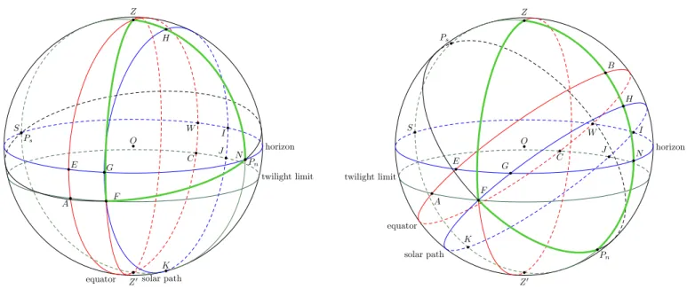
The sphere represents the various circles of interest as seen from a lo-cation at latitude l, the sun being at longitude λ. O is the observer, and NESW is the horizon, with cardinal points N , E, S, and W . The meridian circle is the circle going through N , S, as well as Z (zenith) and Z′ _(nadir).

Pnand Psare the North and South celestial poles, that is, the intersections

of the Earth’s axis with the celestial sphere. All these points are at fixed locations with respect to the observer. The equator is the great circle EBW located halfway between the two poles. The horizon, the meridian and the

(9)

Z Z′ horizon equator solar path twilight limit P_n Ps E A G F W C O I J S N B H K

(10)

mentioned above, owing to the diameter of the sun and refraction, sunrise will occur a little before E and sunset a little after W . This also explains why the days and nights are not equal at the time of equinoxes, but slightly before the spring equinox, and after the autumn equinox. The “equinoxes” are defined as the time when the center of the sun lies on the equator.

During the year, the sun is usually either above, or below the equator, and its path during a day is again a circle. This is of course an approxima-tion, since the sun’s declination is never stationary, and the daily path of the sun is in fact some kind of helix on the celestial sphere. We will how-ever assume that the declination is practically constant during a period of 24 hours. This corresponds to the assumption that the Earth is stationary for one day and somehow progresses stepwise around the sun. We also as-sume that all computations are done in solar time, and not in mean time, thereby ignoring the equation of time (which is anyway constant during a day, owing to our assumption on the declination). All these approxima-tions are the usual ones, see for instance [26, p. 369–370].

In figure 4, the path of the sun is GHI . The sun rises at G (or slightly before), culminates at H, and sets at I (or slightly after). Computing the length of daylight is finding how long it takes the sun to go from G to I.

If we consider nighttime to be when the sun is not visible, then the length of daylight d will immediately yield that of the night n = 24 − d. If we take into account the time of twilight t, then n = 24 − d − 2t, since there are (usually) two twilights. This is made clear on figure 4 where the circle FACJ parallel to the horizon is the limit that the sun has to reach for a given definition of twilight. In that case, at the equinoxes, (morning) twilight will last from A to E, and when the sun’s path is GHI , twilight will correspond to the arcs FG and IJ .

Computing the duration of twilight is computing the length of FG as a fraction of the entire solar path. Again, this discussion is slightly sim-plified in that we have to consider either a point before G, or to assume that the circle we call “horizon” is in fact 50′ _{below the actual horizon.}

In that case, of course, E and W are no longer exactly the East and West directions.

In figure 4, the equator is tilted on the horizon by the colatitude 90◦₋

l. When the latitude is 0◦_{, the poles are at the horizon and the equator}

(11)

situation is reversed in the Southern hemisphere. In addition, when the sun rises in the Southern hemisphere, it does rises at the East, but it then moves towards the North. When the sun culminates, its direction is that of North, and not that of South as in the Northern hemisphere.

The time it takes the sun from G to I is the duration of daylight. The time it takes the sun from F to H is the duration of twilight plus half the duration of daylight. That time is itself proportional to the angle dHPnF

and we can readily see that the computation of twilight involves the reso-lution of two spherical triangles, ZGPn and ZFPn, the latter being shown

in green on figures 4 and 5.

In general, for a spherical triangle ABC with sides (angles) a, b, c and vertex angles A, B, C, we have the relation

cos c = cos a · cos b + sin a · sin b · cos C. (10)

Taking A = Z, B = F and C = Pn, we have (see figure 4)

c= ZF = 90◦_{+ h}

b = ZPn = 90 ◦_{− l}

a= FPn = 90 ◦_{− δ}

where h is the twilight limit (for instance 18◦_{), l is the latitude, and δ is}

the declination of the sun. The declination δ of the sun is itself obtained from its ecliptic longitude λ and from the obliquity ε of the ecliptic with δ = arcsin(sin ε · sin λ).

Equation (10) then becomes:

− sin h = sin δ · sin l + cos δ · cos l · cos dZPnF . (11)

If cos l = 0, that is at each pole, we have − sin h = sin δ, that is, the twilight limit is merely reached when the declination of the sun equals the twilight limit (δ = −h), but since we assume that the declination is constant during a day, there is no specific time associated to this contact.

If cos l 6= 0, we can extract dZPnF:

cos dZPnF = −

sin h + sin δ · sin l cos δ · cos l = −

sin h

cos δ · cos l − tan δ · tan l (12) Using equation (12), we can compute the hour angle for t + d₂, where t

(12)

The angle dZPnF is however not always defined. When l gets closer to

±90◦_{, there is a threshhold, at which the right-hand side of equation (12)}

equals ±1. The same is true for the angle dZPnG. When the daylight

thresh-hold is met, latitudes above or below the threshthresh-hold have either continu-ous daylight, or no daylight at all. When the twilight duration reaches a threshhold, the full duration of twilight is no longer possible.

Computing the threshholds is straightforward. Setting µ = ±1, we have to solve

µ= − sin h

cos δ · cos l − tan δ · tan l (13) hence

µ· cos δ · cos l = − sin h − sin δ · sin l (14) Squaring both sides and solving in sin l, we obtain

sin l = − sin h · sin δ ± cos δ cos h (15)

Once a threshhold has been met for daylight, its duration is either 0 or 24 hours. All these cases have been taken into account for the various figures in this article.

The duration of twilight results in a well-behaved curve as long as twi-light is transient, that is, as long as twitwi-light occurs between daytwi-light and night. Things become more complex if there is no daylight or no night. The “normal” configuration corresponds to latitudes −90◦ _{+ ε + h < l <}

90◦_{− ε − h, where ε is the obliquity of the ecliptic and h is the angle}

corre-sponding to the chosen twilight. For nautical twilight, the twilight curve is nearly circular at the equator and then elongates itself until the latitude reaches 54.5◦ _{(see section 4.2.1). When we come closer to the poles, the}

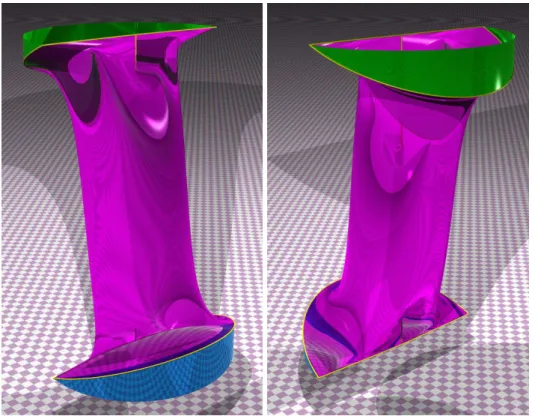
duration of twilight becomes much more intricate and the twilight curve takes on a beautiful flower shape (figure 23).

For a given longitude of the sun, we may also look at the duration of twilight as a function of the latitude, and the variation of twilight is no less interesting (see section 4.3.1).

2.3 Some special cases

(13)

Z

Z′

horizon

equator solar path

twilight limit Pn Ps E A G F W C O I J S N K H Z Z′ horizon equator solar path twilight limit Pn Ps E A G F W C O I J S N B K H

Figure 5: The trigonometry of twilight on the equator (left) and at negative latitudes (right). Z Z′ horizon equator solar path twilight limit Pn Ps E A G W C O S N B H K I Z Z′ horizon equator solar path twilight limit Pn Ps E A W C O S N B H

(14)

When we increase the latitude further, we reach a point where there is no more any twilight (figure 6, right). This happens when l = 90◦_{− δ. We}

then have continuous daylight.

Figure 7 show what happens at the North pole when the solar path is sufficiently far from the equator (and horizon) and from the twilight circle. In the first case (top left), we have continuous daylight. In the second case (top right), we have continuous twilight. And in third case (bottom), we have continuous night. There are however cases where the actual path of the sun crosses the equator circle or the twilight circle, because the dec-lination of the sun does not remain constant. These transitions are not taken into account in our study, because we have always assumed that the declination of the sun is constant over one day.

2.4 The shortest and longest twilights

When given a certain latitude l, we can look for the ecliptic longitude of the sun resulting in the shortest (or longest) twilight. Equation (12) can be used to find for which values of δ the right-hand side is extremal, and then the ecliptic longitude as well as the time of the year can be derived from δ. Since this is not the purpose of this study, we will not examine these questions in detail, but we have given a number of references related to this question. We can however observe that in normal circumstances, that is, when twilight is intermediate between day and night, the longest twilight in the Northern hemisphere takes place at the summer solstice, and the shortest one takes place near the equinoxes.

The question was first raised in 1542 by Pedro Nunes [27]. Johann Bernoulli (1667–1748) and his brother Jacob (1655–1705) are said to have worked on it for five years [6, p. 64], using differential calculus. Many other solutions have been published, some of them purely geometrical. For a recent summary of this question, see Meeus’s discussion [26, p. 368– 379].

(15)

Z Z′ horizon equator solar path twilight limit Pn Ps O S N H K Z Z′ horizon equator solar path twilight limit Pn Ps O S N H K Z Z′ horizon equator solar path twilight limit Pn Ps O S N H K

Figure 7: Top left: continuous daylight at the North pole. Top right: con-tinuous twilight at the North pole. Bottom: concon-tinuous night at the North pole.

(16)

3 Days and nights

Figure 8 shows a 3-dimensional representation of the duration of days d and nights n = 24 − d as a function of the longitude (horizontal plane) and the latitude (vertical axis). The lengths have been scaled down by a factor 5/24 compared to the representation of twilight in figure 23. The parts in green/blue corresponds to a 24-hour day (left) or 24-hour night (right).

Figure 9 shows the duration of the night, excluding the morning and evening twilights. The longer the twilight, the shorter the night, and the shorter the period of permanent day or permanent night. Moreover, the physical area concerned with a permanent day or permanent night also becomes smaller, almost vanishing.

Figure 8: The length of days (left) and nights (right), as a function of the longitude (horizontal plane) and the latitude (vertical axis).

(17)

Figure 9: Night lengths after removal of civil twilight (left), nautical twi-light (center), and astronomical twitwi-light (right).

(18)

3.1 Daylight length for a given longitude

Figures 10 and 11 show the lengths of daylight as a function of the latitude for several longitudes. A few days after the spring equinox, the length of the day at the South pole quickly skips from a permanent day to a perma-nent night. At the summer solstice, the situation has evolved at the North pole, resulting in a kind of 24 hours plateau. At the autumn equinox, the configuration is the same as for the spring equinox.

0 5 10 15 20 25 -80 -60 -40 -20 0 20 40 60 80 day length latitude (a) 0 5 10 15 20 25 -80 -60 -40 -20 0 20 40 60 80 day length latitude (b) 0 5 10 15 20 25 -80 -60 -40 -20 0 20 40 60 80 day length latitude (c) 0 5 10 15 20 25 -80 -60 -40 -20 0 20 40 60 80 day length latitude (d)

(19)

0 5 10 15 20 25 -80 -60 -40 -20 0 20 40 60 80 day length latitude (a) 0 5 10 15 20 25 -80 -60 -40 -20 0 20 40 60 80 day length latitude (b) 0 5 10 15 20 25 -80 -60 -40 -20 0 20 40 60 80 day length latitude (c) 0 5 10 15 20 25 -80 -60 -40 -20 0 20 40 60 80 day length latitude (d) 0 5 10 15 20 25 -80 -60 -40 -20 0 20 40 60 80 day length latitude 0 5 10 15 20 25 -80 -60 -40 -20 0 20 40 60 80 day length latitude

(20)

3.2 Daylight length for a given latitude

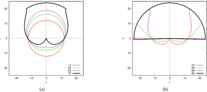
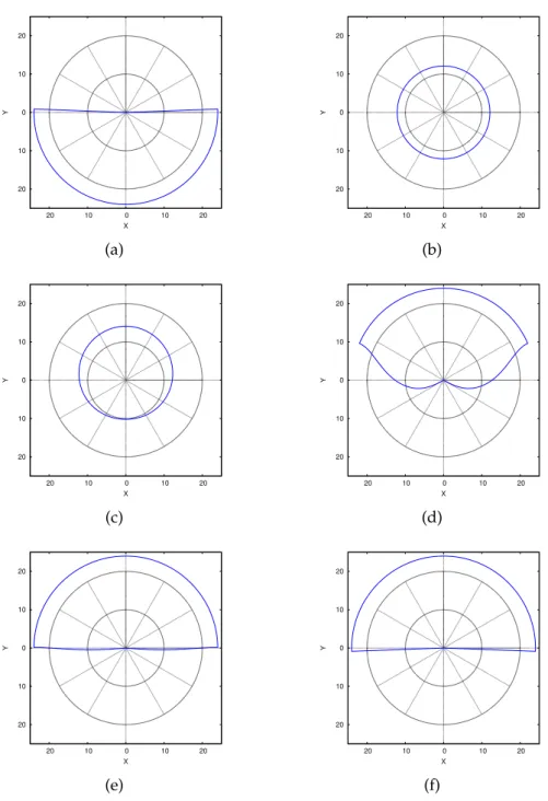
Figure 12 shows two sets of sections (polar representations) of the duration of daylight for several latitudes. These curves are sections of the surface shown in figure 8. Figure 13 shows several sections in isolation. Then, figures 14 and 15 are rectangular representations of the duration of the day, some of them corresponding to the polar representations.

-20 -10 0 10 20 -20 -10 0 10 20 y x 0 50 60 70 (a) -20 -10 0 10 20 -20 -10 0 10 20 y x 70 80 89 90 (b)

Figure 12: Sections of daylight for latitudes 0◦_{, 50}◦_{, 60}◦_{, 70}◦_{, 80}◦_{, 89}◦_{, and}

(21)

20 10 0 10 20 20 10 0 10 20 Y X (a) 20 10 0 10 20 20 10 0 10 20 Y X (b) 20 10 0 10 20 20 10 0 10 20 Y X (c) 20 10 0 10 20 20 10 0 10 20 Y X (d) 20 10 0 10 20 20 10 0 10 20 Y X (e) 20 10 0 10 20 20 10 0 10 20 Y X (f)

(22)

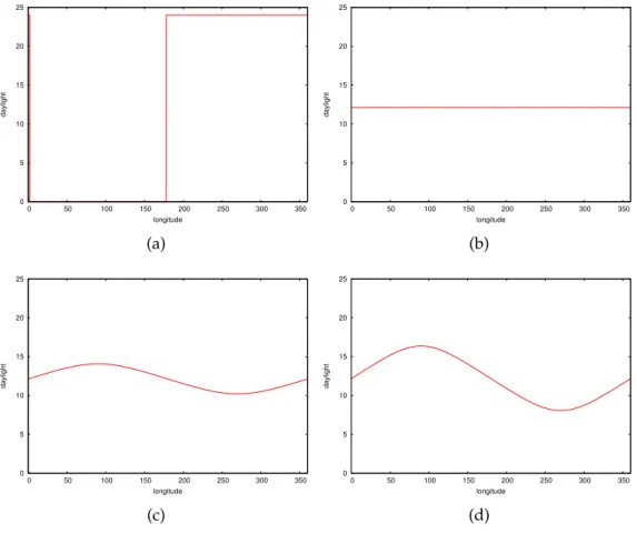
0 5 10 15 20 25 0 50 100 150 200 250 300 350 daylight longitude (a) 0 5 10 15 20 25 0 50 100 150 200 250 300 350 daylight longitude (b) 0 5 10 15 20 25 0 50 100 150 200 250 300 350 daylight longitude (c) 0 5 10 15 20 25 0 50 100 150 200 250 300 350 daylight longitude (d)

Figure 14: The duration of day as a function of longitude, for latitudes −90◦_{, 0}◦_{, 30}◦_{, and 50}◦_.

(23)

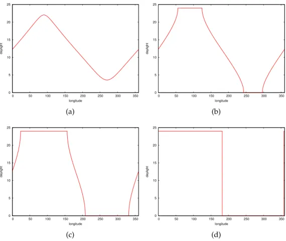
0 5 10 15 20 25 0 50 100 150 200 250 300 350 daylight longitude (a) 0 5 10 15 20 25 0 50 100 150 200 250 300 350 daylight longitude (b) 0 5 10 15 20 25 0 50 100 150 200 250 300 350 daylight longitude (c) 0 5 10 15 20 25 0 50 100 150 200 250 300 350 daylight longitude (d)

Figure 15: The duration of day as a function of longitude, for latitudes 65◦_,

(24)

3.3 Nautical night length for a given longitude

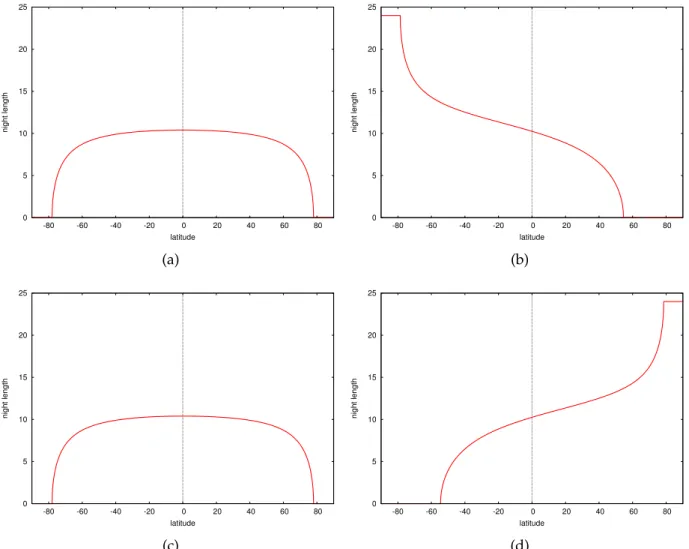
Considering four different positions of the sun, namely those of sunset, of the end of civil twilight, of the end of nautical twilight, and of the end of astronomical twilight, we can define four different nights. The first is merely the time when there is no daylight, and was pictured in figure 8. The three other types of nights are those parts of the first type of night, after the removal of the various twilight times (figure 9). We call there-fore civil night the time from the end of one civil twilight to the start of the next one. Similarly, we call nautical night the time from the end of one nautical twilight to the start of the next one. And finally, we call astronom-ical night the time from the end of one astronomastronom-ical twilight to the start of the next one. In figure 16, we show the nautical night in isolation for the equinoxes and solstices. The configuration is again the same at both equinoxes, where we have seen that there is no night of any kind at both poles.

(25)

0 5 10 15 20 25 -80 -60 -40 -20 0 20 40 60 80 night length latitude (a) 0 5 10 15 20 25 -80 -60 -40 -20 0 20 40 60 80 night length latitude (b) 0 5 10 15 20 25 -80 -60 -40 -20 0 20 40 60 80 night length latitude (c) 0 5 10 15 20 25 -80 -60 -40 -20 0 20 40 60 80 night length latitude (d)

(26)

3.4 Astronomical night length for a given longitude

Figure 17 shows the duration of the astronomical night at the equinoxes and solstices. The durations are similar to those of the nautical length, but the nights are of course shorter than the nautical nights, since by definition they are a part of them. In particular, there are polar regions where 24 hours nautical nights occur, but not 24 hours astronomical nights.

0 5 10 15 20 25 -80 -60 -40 -20 0 20 40 60 80 night length latitude (a) 0 5 10 15 20 25 -80 -60 -40 -20 0 20 40 60 80 night length latitude (b) 0 5 10 15 20 25 -80 -60 -40 -20 0 20 40 60 80 night length latitude (c) 0 5 10 15 20 25 -80 -60 -40 -20 0 20 40 60 80 night length latitude (d)

(27)

3.5 Daylight and nautical night length for a given

longi-tude

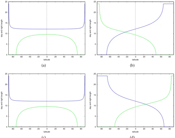
Figure 18 shows the duration of the day and nautical night as a function of the latitude, for the solstices and equinoxes. The durations are the same at both equinoxes when the day is then 24 hours long at both poles, and nautical night is non existent. At the summer solstice, the day is longest at the North pole (blue curve, upper right), and shortest at the South pole (lower left). The situation is reversed at the winter solstice.

0 5 10 15 20 25 -80 -60 -40 -20 0 20 40 60 80

day and night length

latitude (a) 0 5 10 15 20 25 -80 -60 -40 -20 0 20 40 60 80

latitude (b) 0 5 10 15 20 25 -80 -60 -40 -20 0 20 40 60 80

latitude (c) 0 5 10 15 20 25 -80 -60 -40 -20 0 20 40 60 80

latitude

(d)

Figure 18: The length of daylight and nautical night at longitudes 0◦_{, 90}◦_,

(28)

3.6 Daylight and astronomical night length for a given

lon-gitude

Figure 19 now illustrates the duration of daylight and astronomical night together. 0 5 10 15 20 25 -80 -60 -40 -20 0 20 40 60 80

latitude (a) 0 5 10 15 20 25 -80 -60 -40 -20 0 20 40 60 80

latitude (b) 0 5 10 15 20 25 -80 -60 -40 -20 0 20 40 60 80

latitude (c) 0 5 10 15 20 25 -80 -60 -40 -20 0 20 40 60 80

latitude

(d)

Figure 19: The length of daylight and astronomical night at longitudes 0◦_,

(29)

3.7 Daylight isochrones

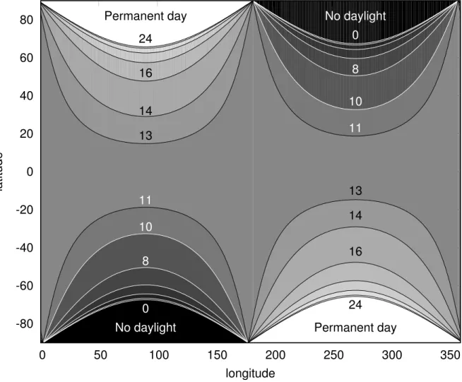
At some point of the year and at some location, the day lasts a certain amount of time. It is interesting to plot the isochrones of daylight and to show at which latitudes and which longitudes the day lasts 10 hours for instance. Superimposing a number of isochrones, we obtain figure 20.2

The horizontal scale gives the longitude of the sun, whereas the verti-cal sverti-cale gives the latitude. Drawing a horizontal line at latitude 40◦_{, for}

instance, shows that at the vernal equinox (longitude 0◦_{), the day lasts}

about 12 hours, then the day increases until about 15 hours at the summer solstice (longitude 90◦_{). It then goes down to about 12 hours at the}

au-tumn equinox (longitude 180◦_{), and continues to decrease reaching about}

9 hours at the winter solstice (longitude 270◦_{), before increasing again until}

the vernal equinox.

The lines marked 0 and 24 give the limits of visibility of the sun. “Per-manent day” means that the sun is visible all day, whereas “No daylight” means that the sun is not visible. That may mean that there is night, de-pending whether we include or not twilight within the night and we have deliberately avoided the term “Permanent night” which is ambiguous. In the white sectors, the day still lasts 24 hours and these sectors are therefore plateaus of sunlight. In the black sectors, the day lasts 0 hours.

Some of these isochrones are shown separately in figures 21 and 22. For each isochrone, there are two parts, one in each hemisphere. These two parts are of course symmetrical. However, one should understand that there is no symmetry around the 12 hours duration and this is exemplified by the 12 hours isochrone. One might expect the 12 hours isochrone to coincide with the equator and we all tend to believe that at the equator the days and nights are equal to 12 hours. This, however, is not totally true, owing to refraction and to the apparent diameter of the sun. If the sun were reduced to a point and there were no atmosphere, the 12 hours isochrone would coincide with the equator, except at the equinoxes where it would cover all latitudes, thus be a vertical line. Instead, at the equator, the days are actually slightly longer than 12 hours, lasting about 12 hours and 7 minutes, plus or minus a few seconds.

We can also observe that for some longitudes a given isochrone may be undefined. There is for instance a slight gap between the Northern and Southern isochrones in figure 21. On the other hand, there is an overlap between the Northern and Southern isochrones in figure 22. The bound-ary between the two families of isochrones is exactly the isochrone

(30)

corre-sponding to the duration of the day at the equator.

Computing the isochrones is based on equation (12) (page 10) which we rewrite for the half day angle dZPnG:

cos dZPnG= −

sin r

cos δ · cos l − tan δ · tan l, (16) rbeing the sunrise angle 50′_.

Each isochrone corresponds to a constant value of dZPnG. If d is the

length of the day in hours, then dZPnG= d

24 × 180◦.

Setting k = cos dZPnG, we solve equation (16). Multiplying by cos δ ·

cos l, we have:

− sin δ · sin l − sin r = k cos δ · cos l (17) The special case k = 0, that is d = 12 hours, is straightforward:

sin l = −sin r

sin δ (18)

Consequently, the 12 hour isochrone is undefined near the equinoxes (δ = 0◦_).

We can also observe that if sunrise were taking place when r = 0◦_{, the}

12 hour isochrone would correspond to l = 0◦_{, hence the equator.}

When k 6= 0, we square equation (17), and solve sin l, obtaining the two equations:

sin l = − sin r · sin δ ± k cos δ p

cos2_r_{− (1 − k}2_{) cos}2_δ

sin2_δ_{+ k}2_cos2_δ (19)

cos l = −sin l · sin δ + sin r

kcos δ (20)

and these are used to determine the latitude as a function of the declina-tion, thus as a function of the ecliptic longitude. In some cases, the right-hand side of the first equation is not in the range [−1, 1], or the right-right-hand side of the second equation is negative or greater than 1, in which case there is no solution for l, meaning that that isochrone is not defined for the given longitude.

(31)

-80 -60 -40 -20 0 20 40 60 80 0 50 100 150 200 250 300 350 latitude longitude Permanent day 24 16 14 13 11 10 8 0 No daylight No daylight 0 8 10 11 13 14 16 24 Permanent day

(32)

-80 -60 -40 -20 0 20 40 60 80 0 50 100 150 200 250 300 350 latitude longitude (a) -80 -60 -40 -20 0 20 40 60 80 0 50 100 150 200 250 300 350 latitude longitude (b) -80 -60 -40 -20 0 20 40 60 80 0 50 100 150 200 250 300 350 latitude longitude (c) -80 -60 -40 -20 0 20 40 60 80 0 50 100 150 200 250 300 350 latitude longitude (d) -60 -40 -20 0 20 40 60 80 latitude -60 -40 -20 0 20 40 60 80 latitude

(33)

-80 -60 -40 -20 0 20 40 60 80 0 50 100 150 200 250 300 350 latitude longitude (a) -80 -60 -40 -20 0 20 40 60 80 0 50 100 150 200 250 300 350 latitude longitude (b) -80 -60 -40 -20 0 20 40 60 80 0 50 100 150 200 250 300 350 latitude longitude (c) -80 -60 -40 -20 0 20 40 60 80 0 50 100 150 200 250 300 350 latitude longitude (d) -80 -60 -40 -20 0 20 40 60 80 0 50 100 150 200 250 300 350 latitude longitude -80 -60 -40 -20 0 20 40 60 80 0 50 100 150 200 250 300 350 latitude longitude

(34)

4 Twilight

4.1 The twilight flower

If we plot the 3-dimensional surface

{(T (l, λ, h) × cos λ, T (l, λ, h) × sin λ, l), −90◦ _{≤ l ≤ 90}◦_,₀◦ _{≤ λ ≤ 360}◦_}

where T (l, λ, h) is the duration of twilight for latitude l, solar longitude λ, and depression h, we obtain the interesting surface of figure 23, here drawn for nautical twilight (h = 12◦_).

The various parts of the surface have been drawn with different colors, and the edges between these parts were drawn in yellow. The middle of this “flower” or “dumbbell” is nearly circular and corresponds to the short twilight at the equator. When we come closer to the poles, the duration of twilight increases, and sometimes reaches its maximal value, whereas at other times it sharply decreases to 0.

Since we have assumed the declination of the sun to be constant over one day, this twilight “flower” is an ideal shape and it would be the shape towards which the actual shape tends if we increase the spinning of the Earth, that is, if we consider the duration of a day very small with respect to the apparent motion of the sun.

(35)

Figure 23: The shape of nautical twilight as a function of the longitude of the sun and of the latitude of the place. The red vector directs towards the longitude 0◦_{, the green vector towards longitude 90}◦_{, and the blue vector}

(36)

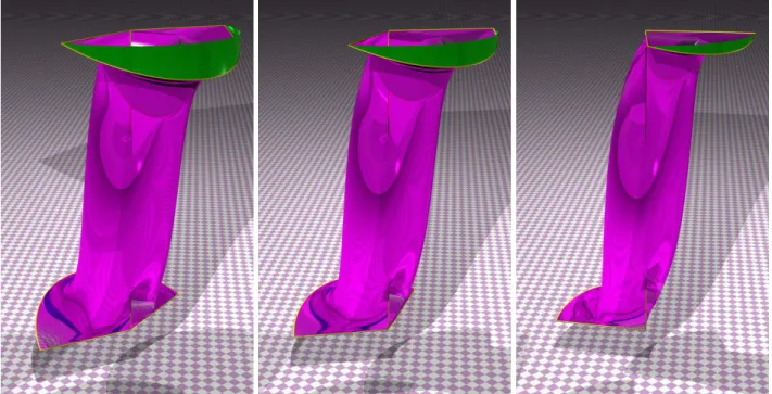
Figure 24: Another view of the nautical twilight flower. The red and ma-genta parts are very intricate.

(37)

(38)

Figure 27: The astronomical twilight flower. The stem is now larger, and so are the periods of maximal twilight.

(39)

(40)

4.2 The variation of twilight for constant latitudes

If we plot the duration of twilight as a function of longitude for increas-ing values of the latitude (figures 29, 30, and 31), a peak appears for the summer solstice (longitude 90◦_).3 _{The peaks increase but at some point the}

shape of the curve changes, because it meets a threshhold. This is readily seen in figure 23 where the summer solstice is in the direction of the green vector. Going up the stem increases the duration of twilight, until we reach the yellow edge. At that point, the duration of twilight can’t extend any-more, and it is also the vanishing of the corresponding night time. One twilight has met the other one. After that point, the duration of twilight drops sharply.

Similar curves would be obtained with negative latitudes, but the peaks would then be located at the winter solstice.

Figures 32 and 33 show the evolution of the three twilights for a range of latitudes from 0◦ _{to 89.9}◦_{. Each twilight meets a first threshhold at the}

summer solstice, which is when the evening twilight meets the morning one, that is when the corresponding night vanishes. The duration of twi-light then decreases, until it reaches 0. The limiting curve is the same for all twilights. When the latitude continues to increase, a second threshhold appears at the winter solstice, and eventually there will be not be any twi-light at the solstices in the polar regions.

3_These _figures _were _suggested _by _figures _produced _by _Irv _Bromberg

(41)

0 0.5 1 1.5 2 2.5 3 3.5 4 0 50 100 150 200 250 300 350 twilight longitude 0 23 30 40 45 50 55 58 59 60 61

(42)

(43)

(44)

0 2 4 6 8 10 12 0 50 100 150 200 250 300 350 twilight longitude 6 12 18 (a) 0 2 4 6 8 10 12 0 50 100 150 200 250 300 350 twilight longitude 6 12 18 (b) 0 2 4 6 8 10 12 0 50 100 150 200 250 300 350 twilight longitude 6 12 18 (c) 0 2 4 6 8 10 12 0 50 100 150 200 250 300 350 twilight longitude 6 12 18 (d) 0 2 4 6 8 10 12 0 50 100 150 200 250 300 350 twilight longitude 6 12 18 (e) 0 2 4 6 8 10 12 0 50 100 150 200 250 300 350 twilight longitude 6 12 18 (f)

(45)

0 2 4 6 8 10 12 0 50 100 150 200 250 300 350 twilight longitude 6 12 18 (a) 0 2 4 6 8 10 12 0 50 100 150 200 250 300 350 twilight longitude 6 12 18 (b) 0 2 4 6 8 10 12 0 50 100 150 200 250 300 350 twilight longitude 6 12 18 (c) 0 2 4 6 8 10 12 0 50 100 150 200 250 300 350 twilight longitude 6 12 18 (d) 0 2 4 6 8 10 12 0 50 100 150 200 250 300 350 twilight longitude 6 12 18 (e) 0 2 4 6 8 10 12 0 50 100 150 200 250 300 350 twilight longitude 6 12 18 (f)

(46)

4.2.1 Nautical twilight for a given latitude

Figures 34 to 39 show sections of the “twilight flower” (figure 23), as well as rectangular representations of the functions.

-6 -4 -2 0 2 4 6 -10 -5 0 5 10 y x (a) 0 2 4 6 8 10 12 0 50 100 150 200 250 300 350 twilight longitude (b) -6 -4 -2 0 2 4 6 -10 -5 0 5 10 y x (c) 0 2 4 6 8 10 12 0 50 100 150 200 250 300 350 twilight longitude (d)

(47)

-6 -4 -2 0 2 4 6 -10 -5 0 5 10 y x (a) 0 2 4 6 8 10 12 0 50 100 150 200 250 300 350 twilight longitude (b) -6 -4 -2 0 2 4 6 -10 -5 0 5 10 y x (c) 0 2 4 6 8 10 12 0 50 100 150 200 250 300 350 twilight longitude (d) -6 -4 -2 0 2 4 6 -10 -5 0 5 10 y x (e) 0 2 4 6 8 10 12 0 50 100 150 200 250 300 350 twilight longitude (f)

(48)

-6 -4 -2 0 2 4 6 -10 -5 0 5 10 y x (a) 0 2 4 6 8 10 12 0 50 100 150 200 250 300 350 twilight longitude (b) -6 -4 -2 0 2 4 6 -10 -5 0 5 10 y x (c) 0 2 4 6 8 10 12 0 50 100 150 200 250 300 350 twilight longitude (d) -6 -4 -2 0 2 4 6 -10 -5 0 5 10 y 2 4 6 8 10 12 twilight

(49)

-6 -4 -2 0 2 4 6 -10 -5 0 5 10 y x (a) 0 2 4 6 8 10 12 0 50 100 150 200 250 300 350 twilight longitude (b) -6 -4 -2 0 2 4 6 -10 -5 0 5 10 y x (c) 0 2 4 6 8 10 12 0 50 100 150 200 250 300 350 twilight longitude (d) -6 -4 -2 0 2 4 6 -10 -5 0 5 10 y x (e) 0 2 4 6 8 10 12 0 50 100 150 200 250 300 350 twilight longitude (f)

(50)

-6 -4 -2 0 2 4 6 -10 -5 0 5 10 y x (a) 0 2 4 6 8 10 12 0 50 100 150 200 250 300 350 twilight longitude (b) -6 -4 -2 0 2 4 6 -10 -5 0 5 10 y x (c) 0 2 4 6 8 10 12 0 50 100 150 200 250 300 350 twilight longitude (d) -6 -4 -2 0 2 4 6 -10 -5 0 5 10 y 2 4 6 8 10 12 twilight

(51)

-6 -4 -2 0 2 4 6 -10 -5 0 5 10 y x (a) 0 2 4 6 8 10 12 0 50 100 150 200 250 300 350 twilight longitude (b) -6 -4 -2 0 2 4 6 -10 -5 0 5 10 y x (c) 0 2 4 6 8 10 12 0 50 100 150 200 250 300 350 twilight longitude (d)

(52)

4.2.2 Astronomical twilight for a given latitude

The general features of the curves are the same as for the nautical twilight, but the theshholds may be advanced or delayed or the amplitudes differ-ent.

As with the nautical twilight, beyond a certain latitude, the duration of twilight can reach its maximal value, namely 12 hours. Since this is actually one of the two twilights, the entire twilight duration will be 24 hours. In other words, the sun will remain between −50′ _{and −18}◦ _{for an}

entire day and at its deepest, it will be below −12◦_.

-10 -5 0 5 10 -10 -5 0 5 10 y x (a) 0 2 4 6 8 10 12 0 50 100 150 200 250 300 350 twilight longitude (b) -10 -5 0 5 10 -10 -5 0 5 10 y x (c) 0 2 4 6 8 10 12 0 50 100 150 200 250 300 350 twilight longitude (d)

(53)

-10 -5 0 5 10 -10 -5 0 5 10 y x (a) 0 2 4 6 8 10 12 0 50 100 150 200 250 300 350 twilight longitude (b) -10 -5 0 5 10 -10 -5 0 5 10 y x (c) 0 2 4 6 8 10 12 0 50 100 150 200 250 300 350 twilight longitude (d) -10 -5 0 5 10 -10 -5 0 5 10 y x (e) 0 2 4 6 8 10 12 0 50 100 150 200 250 300 350 twilight longitude (f)

(54)

-10 -5 0 5 10 -10 -5 0 5 10 y x (a) 0 2 4 6 8 10 12 0 50 100 150 200 250 300 350 twilight longitude (b) -10 -5 0 5 10 -10 -5 0 5 10 y x (c) 0 2 4 6 8 10 12 0 50 100 150 200 250 300 350 twilight longitude (d) -10 -5 0 5 10 y 2 4 6 8 10 12 twilight

(55)

-10 -5 0 5 10 -10 -5 0 5 10 y x (a) 0 2 4 6 8 10 12 0 50 100 150 200 250 300 350 twilight longitude (b) -10 -5 0 5 10 -10 -5 0 5 10 y x (c) 0 2 4 6 8 10 12 0 50 100 150 200 250 300 350 twilight longitude (d) -10 -5 0 5 10 -10 -5 0 5 10 y x (e) 0 2 4 6 8 10 12 0 50 100 150 200 250 300 350 twilight longitude (f)

(56)

-10 -5 0 5 10 -10 -5 0 5 10 y x (a) 0 2 4 6 8 10 12 0 50 100 150 200 250 300 350 twilight longitude (b) -10 -5 0 5 10 -10 -5 0 5 10 y x (c) 0 2 4 6 8 10 12 0 50 100 150 200 250 300 350 twilight longitude (d) -10 -5 0 5 10 y 2 4 6 8 10 12 twilight

(57)

-10 -5 0 5 10 -10 -5 0 5 10 y x (a) 0 2 4 6 8 10 12 0 50 100 150 200 250 300 350 twilight longitude (b) -10 -5 0 5 10 -10 -5 0 5 10 y x (c) 0 2 4 6 8 10 12 0 50 100 150 200 250 300 350 twilight longitude (d)

(58)

4.3 The variation of twilight for constant longitudes

Figures 46 to 49 show a number of configurations in four different cases, with the twilight boundary conditions highlighted in red dashed lines. Each configuration corresponds to a certain latitude l and to a certain dec-lination δ of the sun.

In the first case (figure 46), the declination of the sun is positive, but that case actually applies to all declinations with are greater than the twi-light depression of interest, in other words, it applies to the case δ ≥ −h. The first configuration (a) corresponds to the equator. E is the celestial equator and the blue line is the solar path. In that case, each day has a part of daytime, a part of nighttime, and a part of each of the three proper twilights.

When the latitude increases, there comes a point when the solar path meets the limit of astronomical twilight (figure 46 (c), point 1). In that case, the latitude is exactly 90◦_{− (18}◦_{+ δ). The night then vanishes. When the}

latitude continues to increase, we reach three other threshholds at (d), (e) and (f). These threshholds all correspond to the point of the solar path marked 1.

In the second case (figure 47), we still consider the Northern hemi-sphere, but this time δ ≤ −h. As a consequence, when the latitude in-creases, the contact with the corresponding twilight boundary h occurs on the left side, at point 2 of the solar path. For instance in figure 47 (f), the latitude is 90◦_{+ (18}◦_{+ δ).}

The third and fourth cases (figures 48 and 49) are similar, but for the Southern hemisphere.

In summary, the contacts between the solar path and the twilight boundary h are obtained as follows:

l =          90◦_{− (h + δ),} _{if δ ≥ −h} 90◦_{+ (h + δ),} _{if δ ≤ −h} −90◦_{− (h − δ), if δ ≥ h} −90◦_{+ (h − δ),} _{if δ ≤ h}

Setting p = 1 for the Northern hemisphere and p = −1 for the Southern hemisphere, we can simplify the above cases into:

(59)

E H Pn Ps Z Z′ −18◦ −12◦ −6◦ δ 90◦_{− l} (a) E H Pn Ps Z Z′ δ 90◦_{− l} l (b) E H Pn Ps Z Z′ 1 2 δ 90◦_{− l} l (c) E H Pn Ps Z Z′ 1 2 δ 90◦_{− l} l (d) E H Pn Ps Z Z′ 1 2 δ 90◦_{− l} _l E H Pn Ps Z Z′ 1 2 δ 90◦_{− l} l

(60)

E H Pn Ps Z Z′ δ (a) E H Pn Ps Z Z′ δ l (b) E H Pn Ps Z Z′ 1 2 δ 90◦_{− l} l (c) E H Pn Ps Z Z′ 1 2 δ 90◦_{− l} l (d) E H Pn Z 1 2 _δ l E H Pn Z 1 2 δ l

(61)

E H Pn Ps Z Z′ δ 90◦_{− l} (a) E H Pn Ps Z Z′ δ 90◦_{− l} l (b) E H Pn Ps Z Z′ 1 2 δ 90◦_{− l} l (c) E H Pn Ps Z Z′ 1 2 δ 90◦_{− l} l (d) E H Pn Ps Z Z′ 1 2 δ 90◦_{− l} l E H Pn Ps Z Z′ 1 2 δ 90◦_{− l} l

(62)

E H Pn Ps Z Z′ δ 90◦_{− l} (a) E H Pn Ps Z Z′ δ 90◦_{− l} l (b) E H Pn Ps Z Z′ 1 2 δ 90◦_{− l} l (c) E H Pn Ps Z Z′ 1 2 δ 90◦_{− l} l (d) E H Ps Z 1 2 δ 90◦_{− l} l E H Ps Z 1 2 δ 90◦_{− l} l

(63)

4.3.1 Nautical twilight for a given longitude

Figures 50 to 54 show sections of the “twilight flower” (figure 23) for a number of longitudes. 0 2 4 6 8 10 12 -80 -60 -40 -20 0 20 40 60 80 twilight latitude (a) 0 2 4 6 8 10 12 -80 -60 -40 -20 0 20 40 60 80 twilight latitude (b) 0 2 4 6 8 10 12 -80 -60 -40 -20 0 20 40 60 80 twilight latitude (c) 0 2 4 6 8 10 12 -80 -60 -40 -20 0 20 40 60 80 twilight latitude (d)

(64)

0 2 4 6 8 10 12 -80 -60 -40 -20 0 20 40 60 80 twilight latitude (a) 0 2 4 6 8 10 12 -80 -60 -40 -20 0 20 40 60 80 twilight latitude (b) 0 2 4 6 8 10 12 -80 -60 -40 -20 0 20 40 60 80 twilight latitude (c) 0 2 4 6 8 10 12 -80 -60 -40 -20 0 20 40 60 80 twilight latitude (d) 0 2 4 6 8 10 12 -80 -60 -40 -20 0 20 40 60 80 twilight latitude (e) 0 2 4 6 8 10 12 -80 -60 -40 -20 0 20 40 60 80 twilight latitude (f)

(65)

Figure 52: Nautical twilight for longitudes 90◦_{, 120}◦_{, 140}◦_{, 148.5}◦_{, 160}◦_{, and}

(66)

(67)

Figure 54: Nautical twilight for longitudes 310◦_{, 328.5}◦_{, 350}◦_{, 357.9}◦_{, 358}◦_,

(68)

4.3.2 Astronomical twilight for a given longitude

The duration of astronomical twilight as a function of the latitude has a similar shape as the duration of nautical twilight, and we consider only four longitudes in figure 55.

0 2 4 6 8 10 12 -80 -60 -40 -20 0 20 40 60 80 twilight latitude (a) 0 2 4 6 8 10 12 -80 -60 -40 -20 0 20 40 60 80 twilight latitude (b) 0 2 4 6 8 10 12 -80 -60 -40 -20 0 20 40 60 80 twilight latitude (c) 0 2 4 6 8 10 12 -80 -60 -40 -20 0 20 40 60 80 twilight latitude (d)

(69)

4.3.3 The longitudinal sections of twilight

The following figures give a cumulative view of the three twilights for a number of longitudes. 0 2 4 6 8 10 12 -80 -60 -40 -20 0 20 40 60 80 twilight latitude

(70)

0 2 4 6 8 10 12 -80 -60 -40 -20 0 20 40 60 80 twilight latitude

Figure 57: The length of nautical twilight for various longitudes.

0 2 4 6 8 10 12 twilight

(71)

4.4 Proper twilight

Proper twilight occurs when the sun is located between two given lim-its. For instance, proper civil twilight corresponds to the period when the sun’s depression is between 50′ _{and 6}◦ _{below the horizon. Nautical}

twi-light corresponds to the interval from 6◦ _{to 12}◦ _{and astronomical twilight}

to the interval from 12◦ _{to 18}◦_{. However, as mentioned previously, the sun}

does not always reach these limits. Sometimes it reaches only one of the limits, and sometimes it reaches none. In that case, (half) twilight lasts either 0 hours or 12 hours, and there is in fact either a 24 hours period of continuous twilight of some kind or there is no twilight at all.

4.4.1 Subdivisions of the day

Figures 59 and 60 show the subdivision of the days for various latitudes during the year. Each figure is centered on true noon. At the equator (latitude 0◦_{), there are very little changes during the year and the duration}

of the night, as well as of each proper twilight (in blue, green and red) are almost constant.

The more we increase the latitude, the more differences appear. The days start to increase around the summer solstice and to decrease around the winter solstice. In particular, astronomical twilight (red) becomes longer and longer, and eventually takes up all “night”. Further, proper astronomical twilight vanishes and nautical twilight increases. Eventu-ally, there is no longer any twilight at the summer solstice, only continu-ous daylight. The opposite occurs at the winter solstice, where the days become shorter and shorter as the latitude increases. Eventually the days vanish, with the meeting of the two civil twilights. And then civil twi-light vanishes, and so does astronomical twitwi-light, leaving only continuous night.

The figures 61 and 62 show the same subdivisions, but this time cen-tered on true midnight.

(72)

0 5 10 15 20 0 50 100 150 200 250 300 350 hours longitude (a) 0 5 10 15 20 0 50 100 150 200 250 300 350 hours longitude (b) 0 5 10 15 20 0 50 100 150 200 250 300 350 hours longitude (c) 0 5 10 15 20 0 50 100 150 200 250 300 350 hours longitude (d) 0 5 10 15 20 0 50 100 150 200 250 300 350 hours 0 5 10 15 20 0 50 100 150 200 250 300 350 hours

(73)

0 5 10 15 20 0 50 100 150 200 250 300 350 hours longitude (a) 0 5 10 15 20 0 50 100 150 200 250 300 350 hours longitude (b) 0 5 10 15 20 0 50 100 150 200 250 300 350 hours longitude (c) 0 5 10 15 20 0 50 100 150 200 250 300 350 hours longitude (d) 0 5 10 15 20 0 50 100 150 200 250 300 350 hours longitude (e) 0 5 10 15 20 0 50 100 150 200 250 300 350 hours longitude (f)

(74)

0 5 10 15 20 0 50 100 150 200 250 300 350 hours longitude (a) 0 5 10 15 20 0 50 100 150 200 250 300 350 hours longitude (b) 0 5 10 15 20 0 50 100 150 200 250 300 350 hours longitude (c) 0 5 10 15 20 0 50 100 150 200 250 300 350 hours longitude (d) 0 5 10 15 20 0 50 100 150 200 250 300 350 hours 0 5 10 15 20 0 50 100 150 200 250 300 350 hours

(75)

0 5 10 15 20 0 50 100 150 200 250 300 350 hours longitude (a) 0 5 10 15 20 0 50 100 150 200 250 300 350 hours longitude (b) 0 5 10 15 20 0 50 100 150 200 250 300 350 hours longitude (c) 0 5 10 15 20 0 50 100 150 200 250 300 350 hours longitude (d) 0 5 10 15 20 0 50 100 150 200 250 300 350 hours longitude (e) 0 5 10 15 20 0 50 100 150 200 250 300 350 hours longitude (f)

(76)

4.4.2 Sections of proper twilights

The following figures show the variations of the three proper twilights as a function of the longitude for various latitudes. These figures should be compared with the figures of the previous section.

0 2 4 6 8 10 12 0 50 100 150 200 250 300 350 twilight longitude 6 12 18 (a) 0 2 4 6 8 10 12 0 50 100 150 200 250 300 350 twilight longitude 6 12 18 (b) 0 2 4 6 8 10 12 0 50 100 150 200 250 300 350 twilight longitude 6 12 18 (c) 0 2 4 6 8 10 12 0 50 100 150 200 250 300 350 twilight longitude 6 12 18 (d)

(77)

(78)

(79)

4.4.3 Proper nautical twilight for a given longitude

Figures 66 to 70 show sections of the “proper twilight flower” (figure 72) for a number of longitudes.

The singularities of each curve were computed as described in sec-tion 4.3. The posisec-tions of the singularities depend on the value of the solar declination δ, hence of the value of the longitude. For proper nautical twi-light, we have to consider the singularities resulting from the end of civil twilight (h = 6◦_{) and from the end of nautical twilight (h = 12}◦_{), and we}

have therefore two singularities in each hemisphere. Setting p = 1 for the Northern hemisphere and p = −1 for the Southern hemisphere, we have seen that the latitudes of the singularities are given by:

l = ( p· 90◦_{− (h + pδ), if δ ≥ −p · h} p· 90◦_{+ (h + pδ),} _{if δ ≤ −p · h} 0 2 4 6 8 10 12 -80 -60 -40 -20 0 20 40 60 80 twilight latitude (a) 0 2 4 6 8 10 12 -80 -60 -40 -20 0 20 40 60 80 twilight latitude (b) 0 2 4 6 8 10 12 -80 -60 -40 -20 0 20 40 60 80 twilight latitude (c) 0 2 4 6 8 10 12 -80 -60 -40 -20 0 20 40 60 80 twilight latitude (d)

(80)

(81)

Figure 68: Proper nautical twilight for longitudes 90◦_{, 120}◦_{, 140}◦_{, 148.5}◦_,

(82)

(83)

Figure 70: Proper nautical twilight for longitudes 310◦_{, 328.5}◦_{, 350}◦_{, 357.9}◦_,

(84)

4.4.4 Proper astronomical twilight for a given longitude

The duration of proper astronomical twilight as a function of the latitude has a similar shape as the duration of proper nautical twilight, and we consider only four longitudes in figure 71.

0 2 4 6 8 10 12 -80 -60 -40 -20 0 20 40 60 80 twilight latitude (a) 0 2 4 6 8 10 12 -80 -60 -40 -20 0 20 40 60 80 twilight latitude (b) 0 2 4 6 8 10 12 -80 -60 -40 -20 0 20 40 60 80 twilight latitude (c) 0 2 4 6 8 10 12 -80 -60 -40 -20 0 20 40 60 80 twilight latitude (d)

Figure 71: Proper astronomical twilight for longitudes 0◦_{, 15}◦_{, 90}◦_{, and}

(85)

4.4.5 The proper twilight flowers

Figures 72 and 73 show the proper nautical and astronomical twilight flowers, with the red arrow pointing towards longitude 0◦_{(spring equinox)}

and the green arrow towards longitude 90◦ _{(summer solstice). The proper}

civil twilight flower is identical to the total twilight flower (figure 26). When the depression increases, the polar features of the twilight flower expand (figures 26, 24 and 27) and the period of time concerned by perma-nent twilight increases. The proper twilight flower display these increases in that the two “wings” of the North flower bend further towards the win-ter solstice.

(86)

(87)

5 Future work

Our whole analysis was meant to highlight the hidden beauty within the intricacies of the durations of such apparently mundane notions as day-light, night and twilight. The structure of twiday-light, with its cusps, was likened to a flower, albeit a symmetrical one.

But this flower is an ideal flower, a construction resulting from the as-sumption that the declination of the sun remains constant during a whole day, which is not totally correct. Although this assumption is perfectly reasonable most of the time, it can no longer be maintained when the sun is very close to the horizon, or very close to the twilight circle. In that case, a more accurate calculation should be done, and the actual curves and surfaces should be compared with the ideal ones given in our work.

(88)

6 Bibliography for further research

The following list of references gives the main works related to our subject, as well as a number of solutions to the problem of the shortest twilight. These sources are not exhaustive and are given here only to facilitate fur-ther research.

[1] Henri Andoyer. Cours d’astronomie. Première partie, Astronomie théorique. Paris: J. Hermann, 1923. [3rd edition, pp. 134-137 on twilight].

[2] Torbern Olaf Bergman. Geschichte der Wissenschaften von der Dämmerung. Abhandlungen der Königlichen Schwedischen Akademie der Wissenschaften, 22:237–248, 1762.

[3] Johann Bernoulli. Solutio problematis de minimo crepusculo. Acta Eruditorum anno MDCXCII, page 446, 1692.

[4] Johann Bernoulli. Extrait d’une lettre de M. Bernoulli, Medecin. Journal des Sçavans pour l’année M.DC.XCIII, page 29, 1693. [printed in Paris, reprinted in [6]].

[5] Johann Bernoulli. Extrait d’une lettre de M. Bernoulli, Medecin. Journal des Sçavans, pour l’année M.DC.XCIII, 21:39–40, 1694. [printed in Rotterdam, same as [4], reprinted in [6]].

[6] Johann Bernoulli. Opera omnia, volume 1. Lausanne: Marc-Michel Bousquet, 1742. [p. 64 reprints the article from [4] and [5]].

[7] Jean-Baptiste Biot. Traité élémentaire d’astronomie physique, volume 1. Paris: Bachelier, 1841. [see pp. 309–323 on twilights].

[8] Christophorus Clavius. In sphæram Ioannis de Sacro Bosco commentarius. Rome: Aloisius Zannetti, 1607. [reprinted in [9], pp. 507–557 is a commentary on twilights].

[9] Christophorus Clavius. Operum mathematicorum, volume 3. Mainz: Anton Hierat, 1611. [contains [8]].

(89)

[12] Thomas Stephens Davies. On Bernoulli’s solution of the problem of shortest twilight. The London and Edinburgh philosophical magazine and journal of science, 3(16):277–282, October 1833. [second part].

[13] Joseph Jérôme Lefrançois de Lalande. Astronomie, volume 2. Paris: Veuve Desaint, 1771. [see pp. 713–719 on twilights].

[14] Jean-Baptiste Joseph Delambre. Astronomie théorique et pratique, volume 1. Paris: Veuve Courcier, 1814. [see pp. 339–351 on twilights].

[15] Jean-Baptiste Joseph Delambre. Histoire de l’astronomie du Moyen Âge. Paris: Veuve Courcier, 1819. [see pp. 398–430 on Nunes].

[16] Crépuscule. In Encyclopédie méthodique, mathématiques, volume 1, pages 466–471. Paris: Charles-Joseph Panckoucke, 1784.

[17] Guillaume François Antoine de l’Hôpital. Analyse des infiniment petits, pour l’intelligence des lignes courbes. Paris: Imprimerie royale, 1696. [pp. 52–54 on the shortest twilight, see also [18]].

[18] Jean-Pierre de Crousaz. Commentaire sur l’analyse des infiniment petits. Paris: Montalant, 1721. [p. 155 is a commentary on L’Hôpital [17]]. [19] Johann Heinrich Lambert. Photometria sive de mensura et gradibus

luminis, colorum et umbræ. Augsburg: Wittwe Eberhard Klett, 1760. [see pp. 440–457 on twilights; for the English and French

translations, see [21] and [20]].

[20] Johann Heinrich Lambert. Photométrie, ou de la mesure et de la gradation de la lumière, des couleurs et de l’ombre, 1760. Paris:

L’Harmattan, 1997. [French translation of [19]; see pp. 327–340 on twilights].

[21] Johann Heinrich Lambert. Photometry, or, on the measure and

gradations of light, colors and shade. Illuminating Engineering Society of North America, 2001. [English translation of [19]; see pp. 338–353 on twilights].

[22] Thomas Leybourn. The mathematical questions, proposed in the ladies’ diary, and their original answers, together with some new solutions, volume 4. London: J. Mawman, 1817. [pp. 314–339 give various

(90)

[23] Jean-Baptiste Joseph Liagre. Problème des crépuscules. In Mémoires de l’académie royale des sciences, des lettres et des beaux-arts de Belgique, volume 30, pages 1–41. Bruxelles: Hayez, 1857.

[24] Johann Lulofs. Einleitung zu der mathematischen und physikalischen Kenntniß der Erdkugel. Göttingen: Elias Luzac, 1755. [pp. 70–92 on twilight].

[25] Brian Geoffrey Marsden and R. F. Griffin. The shortest twilight. The Observatory, 120:62–66, 2000.

[26] Jean Meeus. More mathematical astronomy morsels. Richmond, Virginia: Willmann-Bell, Inc., 2002.

[27] Pedro Nunes. De crepusculis liber unus. Lisbon: Ludovicus Rodericus, 1542. [reprinted in [28] and [29]].

[28] Pedro Nunes. Obras, volume 2. Lisboa: Imprensa nacional, 1943. [edition of [27]].

[29] Pedro Nunes. Obras, volume 2. Lisboa: Fundação Calouste Gulbenkian, 2003. [edition of [27]].

[30] Rodolphe Radau. Recherches sur le crépuscule. Le moniteur scientifique, 6:1105–1115, 1864.

[31] Giovanni Battista Riccioli. Almagestum novum, volume 1. Bologna: Heirs of Victor Benati, 1651. [see p. 39 for a summary of values of the twilight angle].

[32] Franz Xaver Stoll. Das Problem der kürzesten Dämmerung. Zeitschrift für Mathematik und Physik, 28:150–156, 1883.

[33] Jean Charles Auguste Vauthier. (La durée du crépuscule). In Histoire et mémoires de l’Académie royale des sciences, inscriptions et belles-lettres de Toulouse. Années 1834, 1835, 1836, volume 4, pages 193–194. Toulouse: Imprimerie de Jean-Matthieu Douladoure, 1837. [34] Karl Zelbr. Ueber das Problem der kürzesten Dämmerung.