HAL Id: inria-00072013
https://hal.inria.fr/inria-00072013
Submitted on 23 May 2006HAL is a multi-disciplinary open access archive for the deposit and dissemination of sci-entific research documents, whether they are
pub-L’archive ouverte pluridisciplinaire HAL, est destinée au dépôt et à la diffusion de documents scientifiques de niveau recherche, publiés ou non,
Andrei Khodakovsky, Pierre Alliez, Mathieu Desbrun, Peter Schröder
To cite this version:
Andrei Khodakovsky, Pierre Alliez, Mathieu Desbrun, Peter Schröder. Near-Optimal Connectivity Encoding of 2-Manifold Polygon Meshes. RR-4575, INRIA. 2002. �inria-00072013�
ISRN INRIA/RR--4575--FR+ENG
a p p o r t
d e r e c h e r c h e
THÈME 2Near-Optimal Connectivity Encoding of 2-Manifold
Polygon Meshes
Andrei Khodakovsky — Pierre Alliez — Mathieu Desbrun — Peter Schröder
N° 4575
Andrei Khodakovsky , Pierre Alliez , Mathieu Desbrun , Peter Schröder Thème 2 — Génie logiciel
et calcul symbolique Projet Prisme
Rapport de recherche n° 4575 — Octobre 2002 —30pages
Abstract: Encoders for triangle mesh connectivity based on enumeration of vertex valences
are among the best reported to date. They are both simple to implement and report the best compressed file sizes for a large corpus of test models. Additionally they have recently been shown to be near-optimal since they realize the Tutte entropy bound for all planar triangulations.
In this paper we introduce a connectivity encoding method which extends these ideas to 2-manifold meshes consisting of faces with arbitrary degree. The encoding algorithm exploits duality by applying valence enumeration to both the primal and dual mesh in a
Andrei Khodakovsky
Department of Computer Science, Caltech akh@cs.caltech.edu
Pierre Alliez
INRIA Sophia-Antipolis pierre.alliez@sophia.inria.fr Mathieu Desbrun
Department of Computer Science, U. of So. Cal. desbrun@usc.edu
Peter Schröder
Department of Computer Science, Caltech ps@cs.caltech.edu
symmetric fashion. It generates two sequences of symbols, vertex valences and face de-grees, and encodes them separately using two context-based arithmetic coders. This allows us to exploit vertex and/or face regularity if present. When the mesh exhibits perfect face regularity (e.g., a pure triangle or quad mesh) and/or perfect vertex regularity (valence six or four respectively) the corresponding bit rate vanishes to zero asymptotically. For triangle meshes, our technique is equivalent to earlier valence driven approaches.
We report compression results for a corpus of standard meshes. In all cases we are able to show coding gains over earlier coders, sometimes as large as 50%. Remarkably, we even slightly gain over coders specialized to triangle or quad meshes. A theoretical analysis reveals that our approach is near-optimal as we achieve the Tutte entropy bound for arbitrary planar graphs of 2 bits per edge in the worst case.
des valences des sommets se sont avérés très compétitifs. De plus il a été récemment dé-montré la proche-optimalité de ces codeurs, en montrant une coïncidence avec l’entropie déduite d’une énumeration de triangulations planaires effectuée par Tutte.
Dans ce papier on introduit une technique de codage de la connectivité qui étend ces idées aux maillages polygonaux. L’algorithme exploite la dualité d’un maillage en générant deux séquences de symboles pour la valence des sommets du maillage primal, puis dual. Ces trains de symboles sont compressés en utilisant un codeur arithmétique contextuel et à modèle adaptatif. Un tel algorithme permet d’exploiter la régularité de face ou de sommet présente dans le maillage, ce qui autorise une entropie proche de zéro asymptotiquement pour des maillages réguliers, et un comportement identique aux algorithmes précédents spécialisés aux maillages triangulaires.
Les résultats sont produits sur un corpus de modèles standards. Dans tous les cas on constate un gain sur les méthodes précédentes, parfois de 50%. Une analyse théorique per-met d’expliquer la proche-optimalité de notre approche en montrant une borne entropique coïncidant avec l’énumeration de graphes planaires, de 2 bits par arête dans le pire des cas.
1
Introduction
Encoding connectivity is an important component (next to geometry coding) of all surface compression algorithms to date. This is true for single rate and progressive coders and independent of the surface primitive, e.g., piecewise linear, NURBS, subdivision, or mul-tiresolution patches.
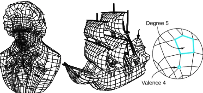
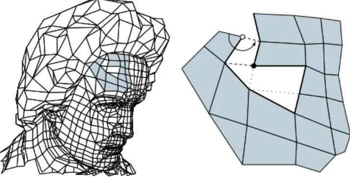
Much of the previous work in this area has been concerned with methods applicable to triangle and quad meshes and has reached some sophistication both in terms of observed and worst case performance. Comparatively little work has been dedicated to the harder problem of connectivity encoding of 2-manifold graphs with arbitrary face degrees and vertex valences (see the examples in Figure1).
Degree 5
Valence 4
Figure 1: Examples of polygon meshes: (left) Beethoven mesh (2812 polygons, 2655 ver-tices) - (right) Galleon mesh (2384 polygons, 2372 verver-tices). Close-up of a polygon mesh: the valence of a vertex is the number of edges incident to this vertex, while the degree of a face is the number of edges enclosing it. Both are in general unconstrained.
Goals and Contributions We propose an extension of the best known single-rate triangle mesh connectivity encoding techniques—which are based on valence enumeration [22,1]— to the encoding of polygon meshes. Our strategy, which is based on encoding all vertex valences and face degrees is near-optimal, i.e., it guarantees the bit rate bound for a planar polygon graph established by Tutte [25] assuming a sub-linear number of split symbols. The implementation of the algorithm is straightforward and its compression performance improves upon all results reported earlier. The latter is true even for coders which are specialized for triangle or quad meshes. Additionally we describe our context-based en-tropy coder which further improves coding performance by exploiting common patterns in meshes.
2
Background and Overview
2.1 Basic Definitions
The specification of a polygon mesh (Figure 1(left)) consists of topologic quantities— vertices, edges, and faces—and geometric quantities—attributes such as vertex positions, face colors, etc. Our interest here is in efficient encoding of topology. Connectivity de-scribes the incidences between elements and is implied by the topology. For example, two vertices or two faces are adjacent if there exists an edge incident to both.
As depicted in Figure1(right), we will call the number of edges incident to a vertex its
valence, while the number of edges incident to a face will be denoted its degree. The ring of
a vertex is the ordered list of all its incident faces. Bit rates will be given in bits per vertex (b/v), bits per edge (b/e), and bits per face (b/f ) as required. The total number of vertices, edges, and faces of a mesh will be denotedV , E, and F respectively.
2.2 Related Work
The related work on single rate coders falls into two major groups of algorithms: those specific to triangle meshes, and those for more general polygon meshes. We review these in turn.
Triangle Meshes Early work was motivated by the desire to render triangle meshes quickly. Deering [5] proposed generalized triangle strips coupled with a vertex cache consuming on average 10 b/v. Bar-Yehuda and Gotsman [2] provided a theoretical study of the cache/compression tradeoff. Speed was also a main concern for Chow [3] and Gumhold [7]. Focusing more on absolute compression ratios, Taubin and co-workers designed the “topological surgery” scheme [20,21] which is capable of adapting to connectivity regularity, resulting in 1 b/v for very regular meshes and 4 b/v on average otherwise.
Subsequently, Rossignac introduced EdgeBreaker [16], a better and simpler traversal technique focusing on edges and introducing the concept of active gate. The mesh is tra-versed by moving to the incident face across an active gate, followed by moving the active gate to the new face. This algorithm has an upper bound of 4 b/v for triangle meshes. A number of improvements to the algorithm [18,19,9,17] and its theoretic bounds [12,19,6] have followed.
In 1998 Touma and Gotsman [22] pioneered a novel vertex-based traversal scheme that provides a natural adaptation to triangle mesh regularity through entropy coding. In contrast to all previous methods, the traversal results inV rather than F tokens, decreasing the bit
recently explained the excellent performance of such algorithms by analyzing the entropy of the list of all valences and showing that it is optimal. There are however exceptional symbols (splits) for which no non-trivial bound is yet known (hence the claim of “near”-optimality). As a practical solution they proposed an adaptive traversal control heuristic which reduces the number of splits to get closer to the optimal bit rate.
Arbitrary Polygon Meshes Given that a polygon mesh with the same number of vertices contains less edges than a triangle mesh it should be possible to encode it with fewer bits. However, initial attempts to compress general graphs [23,11] led to rates of around 9 b/v. These methods are based on building interlocking spanning trees for vertices and faces. Consequently, the number of edges becomes the natural measure of planar graph size, in turn governing the encoding size. Chuang et al. [4] later described a more compact encoding via canonical ordering and multiple parentheses. They state that any simple 3-connected plane graph can be encoded using at most1.5 log2(3)E + 3 ' 2.377 bits per edge.
Li and Kuo [15] pioneered a dual approach that traverses the edges of the dual mesh and outputs a variable length sequence of symbols based on the type of a visited edge. The final sequence is then encoded using a context based entropy encoder.
Isenburg and Snoeyink encoded the connectivity of polygon meshes along with their properties in a method called Face Fixer [10]. This algorithm is gate-based and generalizes the EdgeBreaker algorithm while adding the notion of a face degree. A complete traversal of the mesh is organized through successive gate labeling along an active boundary loop. As in [22,16] both the encoder and decoder need a stack of boundary loops. Seven distinct labels Fn, R, L, S, E, Hn and Mi,k,l are used in order to describe the way to fix faces or
holes together while traversing the current active gate. The labels Fn correspond to face
degrees and are limited to the range [3 − 5] thanks to an additional special symbol Fc.
Since the final sequence of symbols exhibits strong correlation the authors used an order-3 arithmetic coder. King et al. [1order-3] and Kronrod and Gotsman [14] also generalized the EdgeBreaker method to quad meshes and arbitrary polygon meshes respectively. For the latter quad meshes are encoded with3.5 b/v and quadrilateral meshes containing a minority
of triangles with4 b/v. However, none of these polygon mesh encoders come close to the
bit rates of any of the best, specialized encoders [22,1] when applied to triangle meshes.
2.3 Key Concept: Duality
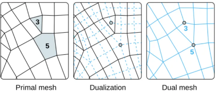
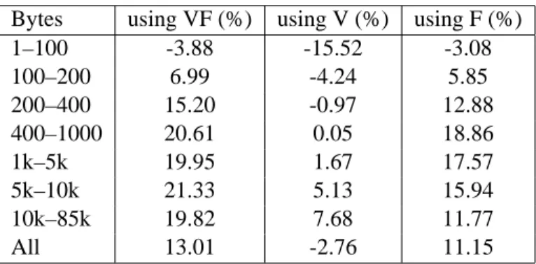
In addition to the previous work analysis, we make the following observation. Consider an arbitrary 2-manifold triangle graphM. Its dual graph ˜M, in which faces are represented as
dual vertices and vertices become dual faces (see Figure2), should have the same connec-tivity entropy: dualization neither adds nor removes information. The valences of ˜M are
now all equal to3, while the face degrees take on the same values as the vertex valences
ofM. Since a list of all 3s has zero entropy, just encoding the list of degrees of ˜M would
lead to the same bit rate as found for the valences ofM. Conversely, if a polygon mesh has
only valence-3 vertices, then its dual would be a triangle mesh. Hence its entropy should be equal to the entropy of the list of its degrees.
3
5
3
5
Primal mesh Dualization Dual mesh
Figure 2: Left: a polygon mesh with highlighted faces of degree 3 and 5. Middle: the dual mesh is built by placing one node in each original face and connecting them through each edge incident to two original faces. Right: the dual mesh now contains corresponding vertices of valence 3 and 5.
The above observation leads us to the key concept of this paper: our compression algo-rithm should be dual, in the sense that both a mesh and its dual get encoded with the same number of bits. As a direct consequence, the encoding process should be symmetric in the coding of valences and degrees. In fact, we will show in the Appendix that encoding each separately realizes the enumeration bound of Tutte. A second direct consequence is that the bit rate of a mesh should be measured in b/e, since the number of edges is the only variable not changing during a graph dualization. However, for purposes of comparison with earlier work we will report comparative results in b/v in Section4.
Note: While this paper was in review, we learned about a similar approach concurrently
developed in independent work by Isenburg [8]. It also exploits the idea of dual mesh en-tropy and lends additional support to the usefulness of this approach. We refer the interested reader to [8] for additional details.
2.4 Overview of our Approach
In this paper, we propose a unified and simple solution for connectivity encoding of tri-angle, quad and polygon 2-manifold meshes with arbitrary topology and any number of components or boundaries.
F6 - V4 - V4 - V4 - V4 - V4 - V4 F4 - V4 - V4 F4 - V4 - V5 F4 - V5 F3 - V4 F4 - V4
F3 - V5 F4 - V4 F4 - V3 - V4 F4 - V5 F4 - V3 - V4 F4 - V5
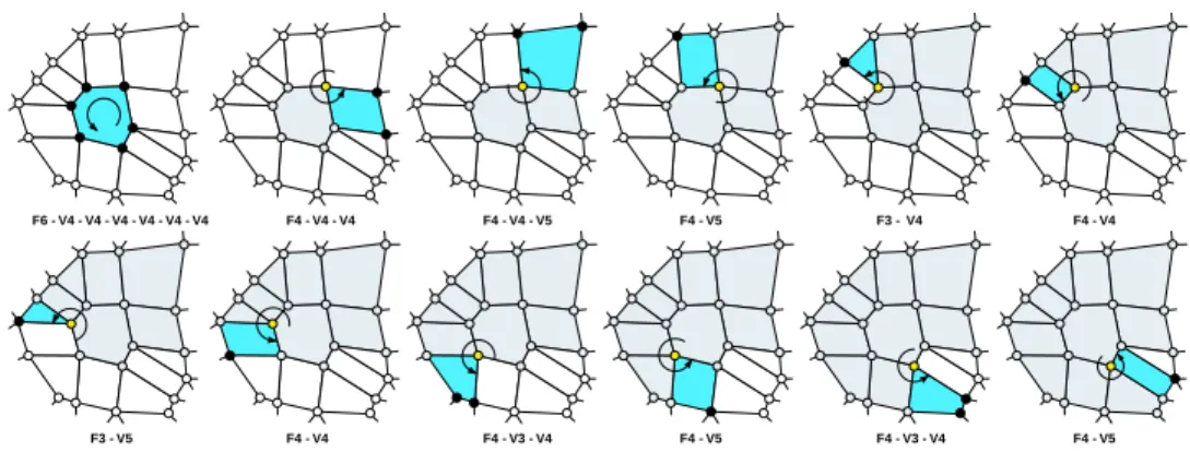
Figure 3: Example of a simple traversal sequence starting from a seed face. At the begin-ning, the seed face degree is output along with the valence of all its vertices. The first vertex then becomes active and the next face is traversed in counterclockwise order, resulting in one face degree and two vertex valences output. The traversal keeps going until all the faces and vertices have been visited.
The basic technique underlying our algorithm is similar to most connectivity compres-sion methods. A seed face is chosen and all its neighbors are traversed recursively until all faces of the corresponding connected component are visited. A new seed face of the next connected component is then chosen and the process continues. Every time the encoder traverses the next element of the mesh, it outputs some symbol which uniquely identifies a new state. From this stream of symbols, the decoder can reconstruct the mesh. Various en-coding algorithms differ in the way they actually traverse a mesh and in the sets of symbols used for identifying the encoder state.
As we have seen in the previous work section, a generalization of the gate-based ap-proach to arbitrary polygon meshes was suggested in [10]. In the present paper we propose a generalization of the second, vertex-based approach. Because of the duality properties of our approach, it may equivalently be viewed as a face-based approach. We use two sets of symbols to encode vertex valences and face degrees. At any given moment both encoder and decoder will know which type of symbol (face or vertex) they are dealing with. Conse-quently, if the input mesh contains only faces of fixed degree (all triangles or all quads, for example), the corresponding stream will be compressed to near zero b/f by an entropy coder leaving only a vertex valence stream. Conversely, if the mesh has faces of varying degrees, but all vertices have the same valence, we get a zero entropy vertex stream. Note that the FaceFixer algorithm also uses face degrees, so it can take advantage of a mesh with uniform
face degrees, but not of one with uniform vertex valences. The shark model exemplifies such a case (see Table2).
3
Encoding Algorithm
In this section we give a complete, yet informal description of our algorithm, including the data structures needed. Pseudo code giving exact details is included in the Appendix. We also discuss the optimality of our approach, and show that encoding both the valence and degree lists exactly matches the worst-case entropy for a planar graph as established by Tutte [25].
Data Structures We maintain only vertex and face data structures explicitly. Vertices store their valence and references to all incident faces in counterlockwise order. Similarly, a face stores its degree and references to all incident vertices in counterclockwise order. Vertices as well as faces go through a sequence of states: empty, active, and complete. At any given time at most one face is active, but there may be multiple vertices active. These are held in the active vertex queue. When a face is processed—moved from empty to active to complete states—all its vertices, which are not yet active, are activated through insertion into the active vertex queue. Consequently, each active vertex has at least one complete incident face. As soon as all the faces incident to a vertex have become complete, the vertex changes its state to complete and is removed from the queue. Thus, the active vertex queue represents the boundary between the part of the mesh which has already been traversed and the part as yet to be visited.
3.1 Traversal Strategy
Initialization step We start the mesh traversal by picking an initial seed face. The encoder outputs the degree of this face, followed by the valences of all the vertices incident to this face in counterclockwise order. These vertices are added to the queue. Conversely, the decoder receives the seed face degree and creates a corresponding face. It then fills all the slots for the incident vertices, moving them from the empty to active state, i.e., enters them into its queue. In this way encoder and decoder maintain matching states.
Completing the vertices The traversal continues by removing the highest priority active vertex from the queue and making it the current vertex. We will discuss heuristics for queue priority assignment in Section3.3.
The algorithm proceeds counterclockwise around the active vertex, skipping all faces which have already been completed. Recall that at least one face is completed and at least one incident face is still empty, otherwise the vertex would not be in the active queue. When the encoder detects an empty face—empty slot in the incident face data structure associated with the current vertex—it proceeds through the following steps:
• the face is activated, it becomes the “current” face, and its degree is output;
• the current face is added to the appropriate slot in the incident face data structures of the current vertex as well as any other active vertices which are incident to current face;
• any remaining empty vertices of the current face are activated and their valences output in counterclockwise order;
• the current face is complete and removed from processing.
Notice that we alternately turn around vertices and faces (see Figure3). The active vertex and the subsequently picked active face can be considered as successive pivots, extending the traversal proposed in [1].
The decoder follows a symmetric procedure, ensuring the same ultimate traversal. When it finds the first empty face slot in the currently active vertex, it proceeds as follows:
• read in a face degree and create the face, moving it from state “empty” to “active,” calling it the “current” face;
• add the current face to the appropriate slot in the active vertex and any other active vertices it is incident on (while the encoder could read off this information the decoder must deduce it and we detail this procedure below);
• read the valences of the remaining empty vertices incident on the current face, acti-vating them through insertion into the active vertex queue;
• move the current face to the complete state.
Any vertices completed during the traversal of the current face are removed from the active vertex queue. They no further belong to the boundary of the traversed region. After the current face is processed the algorithm proceeds to the next face in the currently active vertex until it is complete. Subsequently a new active vertex is taken from the queue and the process repeats until the active vertex queue is empty. If there are some connected components remaining, a new seed face is chosen on it and another component traversal starts.
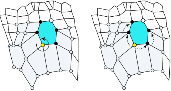
Details of face insertion The procedure that inserts the current face in active vertices other than the current vertex is the only non-trivial operation during the traversal. From the current vertex, we “walk” along the boundary of the visited region in both directions to find which vertices are incident to the current face. The corresponding active vertices will get the current face inserted in their corresponding slots. Since the current face was created to fill the first empty slot in the current vertex we know it shares an edge with the non-empty face slot immediately preceding it in the current vertex (see Figure4for an example). For convenience, let us call the shared edge between these two faces the current edge. It follows that the current face should also be inserted in the active vertex associated with the other end point of the current edge. Further it is known into which face slot in that vertex the current face should be inserted. Iteratively we check whether the preceding face slot in that ring is non-empty. If it is, we update the current edge accordingly and continue as long as we can update the current edge. Once stopped we attempt the same walk in the other direction from the active vertex. Notice that both the encoder and the decoder use the same procedure to find the relevant vertices. Hence the decoder will be able to interpret the subsequent valence transmission(s) with respect to the correct slots in the current face.
Figure 4: Insertion of a face and connection to the existing mesh. First we add the face to the active ring. Next we travel along the boundary adding the new face to all adjacent vertices, first in one direction then in the other. Finally, we insert the remaining (white) vertex based on the valence code received.
Boundaries We deal with boundaries by inserting dummy faces to close every hole of the mesh. The traversal algorithm remains unchanged, and all dummy faces are processed in the same way as regular faces. The only modification is that the valences of dummy faces are encoded using a different symbol so that the decoder can remove them later.
3.2 Splits
Recall that when the decoder creates the current face, all the vertices which can be obtained from neighboring faces are already active. Alas, it is also possible that the current face is incident to an active vertex, without this fact being deducible (see Figure5). We call such a situation a split since locally a single component of the boundary of the visited region is split into two sub-boundaries when this situation occurs. The other possible case is that the unreachable vertex belongs to a different boundary component. Such a situation is usually referred to as a merge [22,1]. Since we only keep a single queue of all boundary vertices without distinguishing between different components, we do not make a distinction between boundary splits and merges. Instead, we refer to both cases as splits, simplifying the implementation.
Splits must happen when encoding non-zero genus models, since a regular traversal always creates regions topologically equivalent to disks. Unfortunately, splits may also occur for models of genus zero. We will see that the traversal order can be optimized to minimize the number of splits.
Figure 5: The black vertex demonstrates the split situation. This vertex already exists in a visited region, but the current (dashed) face cannot find it from its immediate neighbors.
If the encoder detects a split situation, i.e., it is about to activate a vertex which is already active, it outputs a special split symbol instead of the valence. This symbol is followed by the current index of the split vertex in the active vertex queue. The index of the current face in the list of faces incident to the split vertex is also output in order to fully specify the split.
3.3 Heuristic for Traversal Order
Since the split operations are potentially expensive we want to minimize them. Following the approach detailed in [1], we optimize the traversal order by managing the queue
priori-ties based on a heuristic. The priority of each vertex in the queue is inversely proportional to its “incompleteness,” i.e., the number of empty face slots in a ring. This heuristic favors completion of “almost complete” rings. Such rings are usually located in concave sections of the boundary between the visited and non-visited parts of the mesh. Empirically, these are the main source of splits. Hence, the heuristic tends to avoid the formation of such regions, decreasing the number of splits. A number of other heuristics of higher complex-ity were also suggested in [1] and could be used here to achieve potentially better coding performance. To ensure synchronization, both encoder and decoder use the same heuristic.
3.4 Entropy Coding
The output of the traversal algorithm just described consists of a stream of face degree symbols and a stream of vertex valence symbols. These streams could be encoded by any efficient context-based arithmetic coder (AC). Each stream has its own set of context tables. A simple coder can use just one context table per stream. Such a coder is appropriate if the mesh is small or if the encoding stream has a very regular symbol pattern. In general, better encoding results are achieved by using multiple contexts for each stream. Such contexts allow to better exploit both correlations between streams, and between symbols within each stream.
3.4.1 Symbol Definitions
We define 15 symbols for the face degree stream and 16 symbols for the vertex valence stream. Symbols “3”-”15” correspond to actual valences or degrees. The symbol “2” repre-sents valence 2 in the vertex stream and theB(for boundary) symbol in the face stream. The symbol “1” is anESCsymbol for encoding larger valences or degrees. Finally, the symbol “0” is theSplitcode in the vertex stream and is not used in the face stream. BandESC
symbols are followed by the actual degree or valence number (offset, so 16 is mapped to 0). TheSplitsymbol requires the encoding two extra numbers: the index of the split vertex in the active vertex queue and of the current face index in the split vertex. We encode them with a uniform context on the interval[0..N − 1]. For the queue index N is the size of the
queue at that moment. For the index of the current face in the split vertex incident face list,
N is taken to be the number number of empty slots in the split vertex.
If, for a particular stream, only one context is used, the corresponding context table is saved exactly in the file header. In the case when many contexts are used (see below), it is too expensive to save exact tables. Instead, we save only the positions of the most significant bit of all counters. These are used to initialize contexts with approximate distributions.
Tables are then updated by an adaptive arithmetic coder. The cost of encoding a non-empty table is 2-3 bytes on average compared to 10-12 bytes for encoding of an exact table.
3.4.2 Our Statistical Model
The face and vertex streams are encoded using multiple contexts. The appropriate context is chosen based on already-known information about neighboring faces and vertices. This approach is different from using a higher-order arithmetic coder which uses a number of previously processed symbols to define the new context. The latter approach is less advan-tageous, since some of the previous symbols may correspond to faces or vertices which are not relevant to the current symbol.
Face degrees The context for a face degree symbolF is determined by the degree of the
previous faceFp in the same active ring and the sumVav of valences of the vertices on the
edge between the current and the previous faces.
In particular, we separately consider most common degrees 3, 4, 5. IfFphas some other
degree we encode the symbolF with a default context. The same default context is used
when there is no previous face. We use three different contexts for each of degrees 3 and 4 and just one context for a less common degree 5. We decide between three possible contexts depending onVav < Vcrit,Vav = Vcrit,Vav> VcritwhereVcrit= 12 if Fp is a triangle and
Vcrit = 8 if Fpis a quad.
Vertex valences are encoded with 8 contexts in a similar way to face degrees. The context for the vertexV is determined by the degree of the face F which contains this vertex and
the sumVavof valences of all know vertices in that face.
We use three contexts ifF is a triangle or quad, one context for degree 5 and one context
for other degrees. IfF is a triangle or a quad we distinguish between three possible contexts
depending onVav< Nv·Vcrit,Vav== Nv·Vcrit, orVav> Nv·Vcrit, whereNvis a number
of known vertices andVcritis 6 for triangles and 4 for quads.
Discussion The motivation for using such contexts is that the average valence of vertices in quad and triangle regions are different. Therefore, there is a correlation between the vertex or face symbol to encode and the average valence of known neighboring vertices.
We have found the above heuristics to generally improve the coding of meshes. We have experimented our technique on the large SNHC database, and on average, a gain of
13% is observed when we use our simple statistical model over a direct encoding (slightly
contexts based on valences or degrees is consistently worse than our mixed strategy on this 3D database. Although one could adjust this strategy to perform better on a given corpus of meshes, our choice seems a good compromise for the typical meshes used in graphics.
Bytes using VF (%) using V (%) using F (%) 1–100 -3.88 -15.52 -3.08 100–200 6.99 -4.24 5.85 200–400 15.20 -0.97 12.88 400–1000 20.61 0.05 18.86 1k–5k 19.95 1.67 17.57 5k–10k 21.33 5.13 15.94 10k–85k 19.82 7.68 11.77 All 13.01 -2.76 11.15
Table 1: Compression results for the 1296 manifold models from the SNHC database. The results were sorted by the size of the compressed files and averaged by groups. The first column shows the group. The second column shows the relative improvement when using multiple contexts. Third and forth column show improvement when using multiple contexts
only on vertex, and face streams respectively.
3.5 Optimality
Alliez and Desbrun [1] have recently proven that the list of valences of a triangle mesh is an exact entropy measure of connectivity. The worst case scenario fits the theoretical results of Tutte [24] oflog2(256/27) ≈ 3.24 bits per vertex, while regularity in valence leads to
almost zero entropy. In AppendixAwe prove, using a similar approach, that the entropy of the two lists of valences and degrees also matches the counting results of Tutte for general, 3-connected graphs [25]. This proves the “near-optimality” of our approach: under the
assumption that only a sub-linear number of splits is produced during encoding, the bit rate of our encoder is asymptotically optimal. This assumption of a small number of splits holds
for all the meshes we tried. Note though that it is possible to produce “pathological” meshes which will cause a linear number of splits to occur under all heuristics we have considered.
4
Results
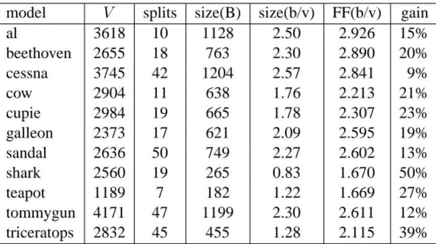
We begin with a performance comparison of our algorithm and the FaceFixer coder. Table2 shows the results of compression for a set of standard models both in total bytes and b/v. The
average improvement is approximately 20%. The most significant improvement is achieved for the shark model: most of the vertices in this model have the same valence. Because of the separation of vertex and face information in our coder, the vertex information was encoded at practically no cost, leading to a factor2 improvement in bit rate performance.
In Tables3and4, we also compare our polygon mesh coder to the Touma-Gotsman (TG) model V splits size(B) size(b/v) FF(b/v) gain
al 3618 10 1128 2.50 2.926 15% beethoven 2655 18 763 2.30 2.890 20% cessna 3745 42 1204 2.57 2.841 9% cow 2904 11 638 1.76 2.213 21% cupie 2984 19 665 1.78 2.307 23% galleon 2373 17 621 2.09 2.595 19% sandal 2636 50 749 2.27 2.602 13% shark 2560 19 265 0.83 1.670 50% teapot 1189 7 182 1.22 1.669 27% tommygun 4171 47 1199 2.30 2.611 12% triceratops 2832 45 455 1.28 2.115 39%
Table 2: Comparison between the FaceFixer algorithm and our approach. The second col-umn shows the number of vertices in the polygon mesh; the third colcol-umn shows the number of splits, the fourth and fifth columns show the size of the compressed file in total bytes and b/v; the sixth column shows the performance of FaceFixer while the last column shows the improvement.
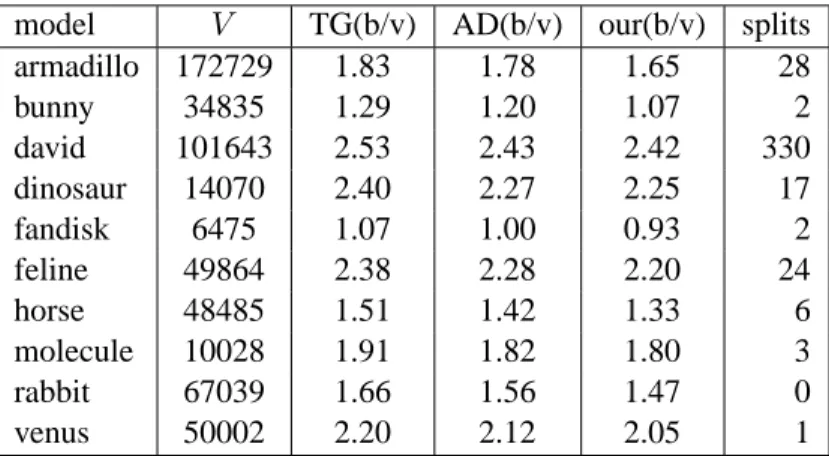
and Alliez-Desbrun (AD) triangle mesh coders on sets of irregular and semi-regular triangle meshes. As expected, all these algorithms exhibit essentially similar performance.
Lastly, we compressed the connectivity of adaptively tessellated Catmull-Clark surfaces (Table 5). These meshes contain mostly quads, but also have a number of “conforming” triangles in the transition regions between different levels of tessellation.
These tables all indicate the better bit rates for polygon meshes, and similar or slightly better results for triangle meshes over the best available coders known as of today. This confirms the notion of near-optimality of our algorithm as proven by our simple entropy analysis. There is however no doubt that it is possible to design better encoders for a specific corpus of meshes by adapting or fine-tuning the statistical modeling we imple-mented. Our current implementation processes all tested meshes in less than two seconds on a PIII 933MHz computer. The set of models we used for comparision can be found at http://www.multires.caltech.edu/software/ircomp
model V TG(b/v) AD(b/v) our(b/v) splits armadillo 172729 1.83 1.78 1.65 28 bunny 34835 1.29 1.20 1.07 2 david 101643 2.53 2.43 2.42 330 dinosaur 14070 2.40 2.27 2.25 17 fandisk 6475 1.07 1.00 0.93 2 feline 49864 2.38 2.28 2.20 24 horse 48485 1.51 1.42 1.33 6 molecule 10028 1.91 1.82 1.80 3 rabbit 67039 1.66 1.56 1.47 0 venus 50002 2.20 2.12 2.05 1
Table 3: The table compares Touma-Gotsman (TG), Alliez-Desbrun (AD), and our com-pression scheme on a number of irregular triangle meshes. The second column shows the number of vertices in the models and the last column shows the number of splits. The coder performances are expressed in b/v.
model V TG(b/v) AD(b/v) our(b/v) splits armadillo 106011 0.020 0.018 0.015 7 bunny 118206 0.019 0.015 0.014 2 dinosaur 129026 0.018 0.015 0.013 4 fandisk 18178 0.061 0.043 0.043 2 feline 258046 0.017 0.013 0.012 17 horse 182274 0.012 0.012 0.010 5 molecule 54272 0.018 0.015 0.013 2 rabbit 107522 0.015 0.013 0.011 0 skull 131074 0.001 0.003 0.001 0 venus 198658 0.012 0.012 0.009 0
Table 4: This table compares Touma-Gotsman (TG), Alliez-Desbrun (AD), and our coder on a number of semi-regular triangle meshes. The second column shows the number of vertices in the models and the last column shows the number of splits. The coder perfor-mances are expressed in b/v.
5
Conclusion and Future Work
We have presented a unified technique for connectivity compression of 2-manifold polygon meshes. It performs near-optimally on all major types of meshes encountered in practice:
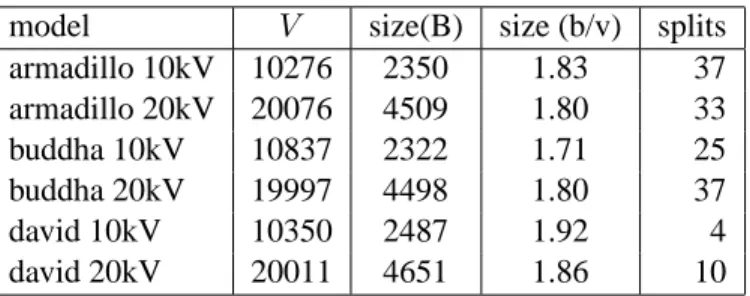
model V size(B) size (b/v) splits armadillo 10kV 10276 2350 1.83 37 armadillo 20kV 20076 4509 1.80 33 buddha 10kV 10837 2322 1.71 25 buddha 20kV 19997 4498 1.80 37 david 10kV 10350 2487 1.92 4 david 20kV 20011 4651 1.86 10
Table 5: The table shows performance of our coder on large adaptively tessellated
Catmull-Clark surfaces. Because of the adaptivity, the meshes contain triangles at the
interfaces between regions of different tessellation depth. The second column shows the number of vertices in the model and the last column shows the numberof splits. The coder performance is expressed in both total bytes and b/v.
triangle, quad and general polygon meshes. Our algorithm exploits duality by encoding separately the list of vertex valences and the list of face degrees. Vertex and/or face regular-ity can therefore be fully exploited. Additionally, we show that encoding these two lists is in perfect agreement with previous theoretical analyses [24,25], and leads to a worst-case of2 b/e on arbitrary meshes, and of 3.24 b/v for triangulations. We also provide a
statis-tical model for the entropy coding that improves compression ratios further by exploiting local regularities in valence and degree distributions. These are found quite commonly in all the meshes we examined. Our implementation demonstrates the compression gains of this polygon mesh compression technique over all previously published techniques, on all tested meshes. The very same algorithm even outperforms most of the previous encoders which were specifically tuned to triangle or quad meshes when applied to such specialized inputs.
Possible future work includes the generalization of this approach to volume meshes, including tetrahedron or hexahedron meshes. This would require vertex, face and edge valences to be encoded. An extension to non-manifold meshes would also be very relevant for practical applications. Finally we hope to build more sophisticated statistical models of valence and degree distributions based on larger corpora of meshes, to further improve the compression performance.
Acknowledgments The work reported here was supported in part by the NSF (ACI-9721349, DMS-9872890, ACI-9982273, EEC-9529152, CCR-0133983). Other support was provided by Intel, Microsoft, Alias|Wavefront, Pixar, and the Packard Foundation.
Craig Gotsman for access to his coder. The datasets are courtesy of Viewpoint Datalabs, Martin Isenburg, Digital Michelangelo Project, Stanford University, Cyberware, Headus, Hugues Hoppe, and The Scripps Research Institute
References
[1] ALLIEZ, P., AND DESBRUN, M. Valence-Driven Connectivity Encoding of 3D Meshes. In Eurographics 2001 Conference Proceedings (Sept. 2001), pp. 480–489. [2] BAR-YEHUDA, R., AND GOTSMAN, C. Time/space Tradeoffs for Polygon Mesh
Rendering. ACM Transactions on Graphics 15(2) (1996), 141–152.
[3] CHOW, M. Optimized Geometry Compression for Real-Time Rendering. In
Visual-ization 97 Conference Proceedings (1997), pp. 347–354.
[4] CHUANG, R. C.-N., GARG, A., HE, X., KAO, M.-Y., AND LU, H.-I. Compact Encodings of Planar Graphs via Canonical Orderings and Multiple Parentheses. In
Automata, Languages and Programming (1998), pp. 118–129.
[5] DEERING, M. Geometry Compression. In ACM SIGGRAPH 98 Conference
Proceed-ings (1995), pp. 13–20.
[6] GUMHOLD, S. New Bounds on the Encoding of Planar Triangulations. Tech. Rep. WSI-2000-1, Wilhelm Schickard Institute for Computer Science, Tübingen, March 2000.
[7] GUMHOLD, S.,ANDSTRASSER, W. Real Time Compression of Triangle Mesh Con-nectivity. In SIGGRAPH 98 Conference Proceedings (1998), pp. 133–140.
[8] ISENBURG, M. Compressing Polygon Mesh Connectivity with Degree Duality Pre-diction. In to appear in Graphics Interface (27-29 May 2002).
[9] ISENBURG, M., AND SNOEYINK, J. Spirale Reversi: Reverse Decoding of
Edge-Breaker Encoding. 12th Canadian Conference on Computational Geometry (2000), 247–256.
[10] ISENBURG, M.,ANDSNOEYINK, J. Face Fixer: Compressing Polygon Meshes With Properties. In ACM SIGGRAPH 2000 Conference Proceedings (2000), pp. 263–270.
[11] KEELER, AND WESTBROOK. Short Encodings of Planar Graphs and Maps.
DAMATH: Discrete Applied Mathematics and Combinatorial Operations Research and Computer Science 58 (1995).
[12] KING, D.,AND ROSSIGNAC, J. Guaranteed 3.67V bit Encoding of Planar Triangle Graphs. 11th Canadian Conference on Computational Geometry (1999), 146–149. [13] KING, D., ROSSIGNAC, J.,ANDSZMCZAK, A. Connectivity Compression for
Irreg-ular Quadrilateral Meshes. Tech. Rep. TR–99–36, GVU, Georgia Tech, 1999.
[14] KRONROD, B., ANDGOTSMAN, C. Efficient Coding of Non-Triangular Meshes. In
Pacific Graphics 2000 Conference Proceedings (october 2000).
[15] LI, J., AND KUO, C.-C. J. Mesh connectivity coding by the dual graph approach, July 1998. MPEG98 Contribution Document No. M3530, Dublin, Ireland.
[16] ROSSIGNAC, J.EdgeBreaker : Connectivity Compression for Triangle Meshes. IEEE
Transactions on Visualization and Computer Graphics (1999), 47–61.
[17] ROSSIGNAC, J., SAFONOVA, A.,ANDSZYMCZAK, A. 3D Compression Made Sim-ple: Edgebreaker on a Corner-Table, 2001.
[18] ROSSIGNAC, J., AND SZYMCZAK, A. Wrap&Zip Decompression of the
Connec-tivity of Triangle Meshes Compressed with EdgeBreaker. Journal of Computational
Geometry, Theory and Applications 14 (november 1999), 119–135.
[19] SZYMCZAK, A., KING, D., AND ROSSIGNAC, J. An EdgeBreaker-based Efficient Compression Scheme for Regular Meshes. 12th Canadian Conference on
Computa-tional Geometry (2000), 257–265.
[20] TAUBIN, G., HORN, W., LAZARUS, F.,ANDROSSIGNAC, J. Geometry Coding and VRML. Proceedings of the IEEE 96(6) (1998), 1228–1243.
[21] TAUBIN, G., AND ROSSIGNAC, J. Geometric Compression Through Topological
Surgery. ACM Transactions on Graphics 17, 2 (April 1998), 84–115.
[22] TOUMA, C., AND GOTSMAN, C. Triangle Mesh Compression. Graphics Interface
98 Conference Proceedings (june 1998), 26–34.
[23] TURAN, G. Succinct representations of graphs. Discrete Applied Mathematics 8
[24] TUTTE, W. A Census of Planar Triangulations. Canadian Journal of Mathematics 14
(1962), 21–38.
[25] TUTTE, W. A Census of Planar Maps. Canadian Journal of Mathematics 15 (1963),
249–271.
A
Entropy Analysis
Consider a 2-manifold polygon meshM with V vertices, E edges, and F faces, and the
following standard assumptions on the mesh:
• it has no boundary, i.e., every edge has two incident faces; • it is topologically equivalent to a sphere, i.e., has genus zero; • it has only one connected component.
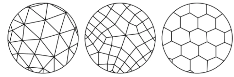
For the sake of clarity, we also definer to be the ratio between the number of faces and the
number of vertices,r = F/V . Typical examples for r are 2, 1 and 0.5 for triangle, quad
and hex meshes respectively (see Figure6). If a mesh has no digon, no stick and no isolated vertex,r lies in the range [0.5, 2].
Figure 6: Left: a triangle mesh (r = 2), average vertex valence 6. Middle: a quad mesh
(r = 1), average vertex valence 4. Right: a hex mesh (r = 0.5), vertex valence 3.
Entropy of a degree sequence
The entropy is a measure of the information content of a series of symbols. More precisely, it denotes the minimal number of bits per symbol required for lossless encoding of the sequence. It is both a function of the numberN of distinct symbols and their respective
probabilitiespi entropy= N X pi log2 1 p .
The final bit rate of a connectivity encoding technique is therefore intimately related to the statistical distribution of the symbols used.
Next, we review the constraints on the distribution of vertex valences and face degrees in an arbitrary polygon mesh.
Euler formula
Euler’s formula for a 2-manifold polygon mesh of genus zero, one connected component and no boundary states:
F + V − E = 2. (1)
Additional relations between the number of edges,E, vertex valences, and face degrees,
are: N X i=3 vi= 2E and M X j=3 fj = 2E.
These simply state that summing all valences, respectively degrees, counts each edge twice. These sums may be rewritten by summing the number of times each valence or degree occurs. This is most conveniently expressed through the use of probabilities of occurrence of each valence and degree. Let the former be given bypi fori = 3, . . . , ∞ and the latter
byqjforj = 3, . . . , ∞ to give: V ∞ X i=3 i pi= 2E and F ∞ X j=3 j qj = 2E. (2)
Solving Eq.1forE, substituting into Eqs.2, dividing byV and F respectively we arrive at
the following expressions for the average vertex valences and face degrees:
¯ v = ∞ X i=3 i pi= 2E V = 2(r + 1), ¯ f = ∞ X j=3 j qj = 2E F = 2( 1 r + 1), (3)
where the last equalities hold in the limit asV and F go to infinity. Note that these equations
Worst asymptotic bit rate vs. Tutte’s enumeration
The algorithm described in this paper encodes both the vertex valence list and the face degree list. The entropy of the valences is:
eV = ∞
X
i=3
pi log2(1/pi) [b/v],
while that for the degrees is:
eF = ∞
X
j=3
qj log2(1/qj) [b/f].
Multiplying through by the ratiosV /E and F/E found in Eq.3one can express the total
bit ratee, i.e., the sum of both bit rates, in units of b/e:
e = 1 r + 1eV + r r + 1eF = ∞ X i=3 pilog2(1/pi) + r ∞ X j=3 qjlog2(1/qj) r + 1 . (4)
Our goal in the remainder of this section is to find the maximum possible entropy e
for arbitrary meshes withr ∈ [0.5, 2]. Maximizing Eq.4 each as a function ofpi andqj
without any additional constraints would lead to both a maximum number of distinct face degrees and vertex valences, each with an equal probability of occurrence. However, such a configuration of valences and degrees is incompatible with Euler’s formula. This leads us to a constrained maximization problem.
There are a total of four constraints on thepiandqj. Two are given by Eq.3with two
additional constraints simply stating that thepiandqj have to sum to one: ∞ X i=3 pi = 1 and ∞ X j=3 qj = 1. (5)
Incorporating these constraints through the use of Lagrange multipliers as was done in [1], the maximation of Eq.4can be achieved by choosingpiandqj to maximize:
f (p3, p4, . . . , λp, µp, q3, q4, . . . , λq, µq) = 1 r + 1 ∞ X 3 pi log2 1 pi + λp( ∞ X 3 pi− 1) + µp( ∞ X 3 i pi− 2(r + 1))+ r r + 1 ∞ X 3 qj log2 1 qj + λq( ∞ X 3 qj− 1) + µq( ∞ X 3 i qj− 2( 1 r + 1)),
whereλp,µp, λq andµq are the four Lagrange multipliers. Equating all derivatives off
with respect to each of the unknown variablespiandqj to zero, we find thatpiandqjmust
follow an exponential decay:
pi = αv β −i
v and qj = αf β −j f .
To determine the coefficientsαv,αf,βv, andβf, we rewrite the constraints given by Eqs.5
and3as: ∞ X i=3 pi = αv ∞ X 3 β−i v = 1 ∞ X j=3 qj = αf ∞ X 3 β−j f = 1 ∞ X i=3 i pi = αv ∞ X 3 i β−i v = 2(1 + r) ∞ X j=3 j qj = αf ∞ X 3 j β−j f = 2( 1 r + 1).
Using the identities (valid forβ > 1):
∞ X i=3 β−i = β −2 β − 1 ∞ X i=3 i β−i = 3β − 2 β2(β − 1)2,
we find the following unique solution:
αv =
4 r2
(2 r − 1)3, and βv = 2 r 2 r − 1,
αf =
4 r
(2 − r)3, and βf = 2 2 − r.
Substituting these solutions leads to the worst-case bit rate functione(r) plotted in Figure7.
0 0.5 1 1.5 2 2.5 0.5 1 1.5 2 (r)
bit-rate (bits per edge)
Figure 7: Plot of the worst-case bit ratee(r) in units of b/e.
As seen in the figure, and as easily proven by studying the derivatives of the entropy curve, the maximum bit rate is reached forr = 1 :
e(1) = −ln(4)
ln(2) + 4 = 2 [b/e].
This coincides exactly with the minimum number of bits needed to encode each edge of an arbitrary planar graph found by Tutte [25] through enumeration of all possible genus-0 3-connected graphs. The fact that we meet the exact entropy of general polygon meshes validates a posteriori our approach of encoding independently the valence and degree lists. This, by no means, should be confused with a claim of optimality for a given corpus of meshes: it simply means that over the whole set of polygon meshes, one can not hope to devise a connectivity algorithm requiring a smaller maximum number of bits. As we mentioned in Section4, better algorithms could be designed for a restricted set of meshes.
Notice thate(2) = 1.08 b/e ' 3.24 b/v for a triangle mesh, exhibiting the upper bound
oflog2(256/27) b/v proven by Tutte from the enumeration of planar triangulations [24].
The maximum entropy is the same whenr = 0.5, confirming our remark that a mesh and its
dual should have the same entropy. Meshes for whichr = 0.5 are duals of triangle meshes.
More generally, we observe thate(r) = e(1/r), i.e., primal and dual meshes have equal
B
Pseudo-code of our traversal algorithm
In the following pseudo-code we use a Face class and a Vertex class such as each face has access to its degree and to an array of its vertices, and each vertex has access to its valence and an array of its adjacent faces. We further assume that any access to a vertex (resp., face) array is done modulo the degree (resp., the valence), to avoid unnecessary index testing. “ActiveSet” is a container for all active vertices. Finally, the following functions have to be implemented in the decoder and the encoder to perform actual I/O operations (read for the decoder, write for the encoder):
Face* ioFace (v, j) – i/o a degree. Returns a face
Face* ioFaceInit () – likewise, but just to bootstrap. Returns 0 if Done
Vertex* ioVertex (f,i) – i/o a valence or a Split code. Returns Vertex or 0 (if split) int ioSplitVertex (f,i) – i/o a vertex index in ActiveSet,
int ioSplitPos (f,i); – i/o a face position in a vertex array //Entry point
void run ( ) {
while ( runComponent ()! = Done ) ;
}
//Process one connected component
Result runComponent ( ) {
if ( ! init () ) return Done; while ( v=ActiveSet.next () ) { completeV (v); ActiveSet.remove (v); } return Continue; }
//Initialization, returns false if the whole mesh is processed
bool init ( ) {
if ( ! f = ioFaceInit () )
return false; //all faces are processed
for ( i = 0 ; i< f.degree ; i++ )
activateV (f, i); //process all vertices
}
//Completes processing of the current vertex.
//in: v has valid valence and v.f[0] fields
//out: all fields of v are valid
void completeV ( v ) {
while ( j = v.firstEmpty () ) { //while there is an empty slot
f = activateF (v, j); //create a face
completeF (f, j); //process its vertices
} }
//Consistency of a face-vertex state (“FV”) means:∀ i: f.v[i] == v =⇒ ∃ j: v.f[j] == f
//“Linked edge” consistency means:
//∀ j: (v.f[j] ! = 0 && v.f[j-1] ! = 0) =⇒ ∃ i1, i2: v.f[j].v[i1+1] == v.f[j-1].v[i2-1]
//Creates a face
//in: vertex v and face’s position j
//out: active face (degree and f.v[0] are valid), f is “FV” consistent with v
void activateF ( v, j ) {
f = ioFace (v,j); //i/o degree, create face
f.v[0] = v;
addFaceToVertex (f, 0, v, j);
}
//Create a vertex
//in: a face and vertex’s position i
//out: an active vertex (valence and v.f[0] are valid), f is “FV” consistent with v
void activateV ( f, i ) {
v = ioVertex (f, i); //i/o valence (creates a vertex) or Split
if ( v ) { //if a new active vertex
f.v[i] = v; v.f[0] = f; ActiveSet.add (v);
} else { //vertex already exists: Split
v = ioSplitVertex (f, i); //i/o v’s index in ActiveSet, returns v
j = ioSplitPos (f, i); //i/o position of f in v
addFaceToVertex (f, i, v, j);
}
return v;
}
//Processes all vertices of a face f
//in: an active face f (degree and f.v[0] are valid), and face’s position j> 0, (v.f[j-1] ! = 0)
//out: all fields of f are valid, “FV” is enforced
void completeF ( f, j ) {
vp = f.v[0]; jp = j; i = 1;
while ( vn = f.v[i] ) { //forces “FV” in “next” direction
jn = vn.find ( vp.f[jp-1] )-1; vn.addFaceToVertex (f, i, vn, jn); vp = vn; jp = jn; i++; if ( i>= f.degree ) return ; } ilast = i; vp = f.v[0]; jp = j; i = f.degree -1;
while ( vn = f.v[i] ) { //forces “FV” in “prev” direction
jn = vn.find ( vp.f[jp+1] )+1;
addFaceToVertex (f, i, vn, jn);
vp = vn; jp = jn; i- -;
if ( i<= ilast ) return ;
}
for ( ; ilast< i; ilast++ ) //process unresolved vertices activateV (f,ilast);
}
//Adds face f to a vertex v
//in: face f and vertex v, f.v[i] == v, an index j
//out:v.f[j] == f, “link edge” is enforced on v
void addFaceToVertex ( f, i, v, j ) {
v.f[j] = f; //add a face
if ( fp = v.f[j-1] ) { //if prev face exist “link edge”
ip = fp.find (v);
if ( ! f.v[i+1] )
}
if ( fn = v.f[j+1] ) { //if next face exist “link edge”
in = fn.find (v);
if ( ! f.v[i-1] )
f.v[i-1] = fn.v[in+1]; }
615, rue du Jardin Botanique - BP 101 - 54602 Villers-lès-Nancy Cedex (France)
Unité de recherche INRIA Rennes : IRISA, Campus universitaire de Beaulieu - 35042 Rennes Cedex (France) Unité de recherche INRIA Rhône-Alpes : 655, avenue de l’Europe - 38330 Montbonnot-St-Martin (France) Unité de recherche INRIA Rocquencourt : Domaine de Voluceau - Rocquencourt - BP 105 - 78153 Le Chesnay Cedex (France)