Blade dynamics in combined waves and current
The MIT Faculty has made this article openly available. Please share how this access benefits you. Your story matters.Citation Lei, Jiarui and Heidi Nepf. "Blade dynamics in combined waves and current." Journal of Fluids and Structures 87 (May 2019): 137-149 © 2019 Elsevier Ltd
As Published http://dx.doi.org/10.1016/j.jfluidstructs.2019.03.020
Publisher Elsevier BV
Version Author's final manuscript
Citable link https://hdl.handle.net/1721.1/126720
Terms of Use Creative Commons Attribution-NonCommercial-NoDerivs License
Blade dynamics in combined waves and current 1
2
Jiarui Lei1, Heidi Nepf1 3
1Department of Civil and Environmental Engineering 4
Massachusetts Institute of Technology, Cambridge, Massachusetts, United States 5
Corresponding author: Jiarui Lei ([email protected]) 6
7
Key points (Highlights): 8
1. A new prediction of drag on a flexible blade in combined wave and current is derived 9
and validated with experiments. 10
2. The drag on a flexible blade in waves decreases with increasing current magnitude. 11
3. The limits of wave-dominated and current-dominated drag are defined. 12
13
Keywords: Reconfiguration; fluid-structure interaction; combined wave-current; flexible 14
vegetation; effective length 15
16
Abstract 17
Submerged aquatic vegetation (SAV), such as seagrass, is flexible and reconfigures 18
(bends) in response to waves and current. The blade motion and reconfiguration modify 19
the hydrodynamic drag. The modified drag can be described by an effective blade length, 20
𝑙𝑒, which is defined as the length of rigid blade that results in the same drag as a flexible 21
blade of length 𝑙. In many natural settings SAV is exposed to combinations of waves and 22
current. This study derived and used laboratory measurements to validate new 23
predictions of effective blade length for combined waves and current based on a Cauchy 24
number, which describes the ratio of hydrodynamic drag to the blade restoring force due 25
to rigidity. Force measurements on and digital images of blades exposed to waves with a 26
2-s period and with a range of wave velocity (𝑈𝑤) and current speed (𝑈𝑐) were used to 27
estimate the effective blade length. The measurements were also used to validate a 28
numerical simulation of blade motion. Once validated, the simulation was used to expand 29
the investigated parameter space to a wider range of wave conditions, and in particular 30
longer wave periods. For 𝑈𝑐 < 1
4𝑈𝑤, the blade motion and hydrodynamic drag were wave-31
dominated. For 𝑈𝑐 > 2𝑈𝑤, the blade motion and hydrodynamic drag were current-32
dominated. 33
1 Introduction 35
Submerged aquatic vegetation (SAV) provides many ecosystem services (Barbier et 36
al., 2008). They are important habitats and shelter areas for fish and shellfish, and 37
supply food for herbivorous animals such as dugong, manatees and sea turtles 38
(Costanza et al. 1997, Waycott et al. 2005). Seagrass, a common marine SAV, is a 39
significant global carbon sink, sequestering more carbon per hectare than rainforests 40
(Fourqurean et al., 2014). Other studies have shown that SAV can protect shorelines 41
from erosion by attenuating wave energy (e.g. Bradley & Houser 2009, Infantes et al, 42
2012, Arkema et al. 2017). Understanding wave attenuation by SAV would be useful in 43
predicting coastal protection provided by SAV and for understanding how SAV 44
promotes particle retention and carbon sequestration. 45
Many previous studies have characterized the damping of waves by vegetation, both 46
using model vegetation in the lab (e.g. Mendez & Losada 2004, Augustin et al. 2009, 47
Stratigaki et al. 2011) and through field studies (e.g. Bradley & Houser 2009, Paul & 48
Amos 2011, Infantes et al. 2012). Some of these studies have accounted for the 49
flexibility of the vegetation. For example, Mullarney and Henderson (2010) developed 50
an analytical model based on cantilever beam theory to simulate the movement of 51
single-stemmed vegetation, such as sedges. The model predicted that wave damping 52
by flexible vegetation was just 30% of that for rigid vegetation. Houser et al. (2015) 53
investigated the dependence of the drag coefficient on blade flexibility, and, similar to 54
Mullarney and Henderson (2010), they found that drag force was reduced with 55
increasing blade flexibility. 56
In many natural settings, SAV is exposed to waves and current together (e.g. 57
Ysebaert et al. 2011), but only a handful of studies have considered the impact of 58
current on wave damping by vegetation. Li and Yan (2007) used a three-dimensional 59
RANS model and Hu et al. (2015) used a laboratory study to show that current flowing 60
in the direction of wave propagation enhances wave dissipation. However, both studies 61
only considered rigid vegetation. Paul et al. (2012) conducted flume experiments with 62
flexible model vegetation and observed the opposite trend, i.e. the presence of current 63
reduced the wave dissipation. Losada et al. (2016) performed laboratory experiments 64
using real vegetation and found that wave damping was enhanced by current flowing in 65
the opposite direction, but was reduced by current in the same direction as wave 66
propagation. Losada et al (2016) proposed a new description for wave damping that 67
accounted for the blade deflection by the current. Specifically, in the description of wave 68
energy dissipation the full blade length, 𝑙, was replaced by the measured deflected 69
height, ℎ𝐷, defined as the vertical distance between the time-mean position of the blade 70
tip and the bed. This paper will build on the work of Losada et al (2016), by providing a 71
way to predict the deflected height, a priori, rather than relying on measured ℎ𝐷. Further, 72
this paper develops a model to predict the hydrodynamic drag on a single flexible blade 73
interacting with combined waves and current by considering how flexible blades move in 74
response to water motion. The new model can form the basis for predicting wave 75
energy dissipation. 76
Luhar and Nepf (2011, 2016) defined an effective blade length, 𝑙𝑒, to characterize 77
the impact of reconfiguration on the drag force on an individual blade in unidirectional 78
flow and in waves. The effective length is defined as the length of a rigid blade that 79
experiences the same drag as a flexible blade of length 𝑙. Generally, reconfiguration 80
reduces drag, such that 𝑙𝑒 < 𝑙. The reduction in drag is associated with the reduction in 81
plant frontal area as well as the streamlining of the blade, and for wave conditions, the 82
motion of the blade reduces the relative velocity between the blade and the water. The 83
effective blade length provides a way to modify models that predict wave damping for 84
rigid stems to predict wave damping by flexible stems. Dalrymple et al. (1984) derived a
85
wave decay coefficient, 𝐾𝐷, for linear waves propagating through a meadow of
86
vegetation consisting of an array of rigid blades of length 𝑙.
87 𝐾𝐷 = 2 9𝜋𝐶𝐷𝑎𝑣𝑘 ( 9 sinh(𝑘𝑙)+ sinh(3𝑘𝑙) sinh 𝑘ℎ (sinh(2kh)+ 2𝑘ℎ )) (1) 88
Here, 𝑎𝑣 is the plant frontal area per meadow volume, 𝑘 is the wave number and ℎ is 89
the water depth. Lei and Nepf (2019) demonstrated that eqn. (1) predicts wave decay 90
over a flexible meadow, if 𝑙 is replaced with 𝑙𝑒, with 𝑙𝑒 described by scaling laws 91
developed for individual blades in pure waves (Luhar and Nepf, 2016). The present 92
paper builds on this concept by developing scaling laws for 𝑙𝑒 that apply to conditions 93
with combined waves and current. To facilitate the discussion, we review the scaling 94
laws previously developed for blades in pure current and in pure waves in section 2. 95
This study seeks to extend the concept of effective blade length to conditions 96
with combined waves and current. First, building on existing scaling laws for pure 97
current and pure waves (described below), a new scaling law is proposed for 𝑙𝑒⁄ under 𝑙 98
conditions with combined waves and current. Second, the new formulation is tested 99
using measured and simulated drag forces on individual model blades. Finally, digital 100
video images are used to examine the blade motion in greater detail to support the 101
description of the scaling laws. 102
103
2 Scaling Laws for Blades in Combined Wave and Current Conditions 104
The change in blade posture in response to water motion, called reconfiguration 105
(Figure 1), can be described by the three dimensionless parameters (e.g. Luhar and 106
Nepf 2011, 2016). First, the Cauchy number, shown in eqn. (2), is the ratio of 107
hydrodynamic drag to the restoring force due to blade stiffness. As shown in eqn. (2), 108
the Cauchy number has a different definition in pure current (𝑈𝑐), denoted 𝐶𝑎𝑐, and in 109
pure wave (𝑈𝑤), denoted 𝐶𝑎𝑤. Second, the buoyancy parameter, 𝐵, is the ratio of 110
restoring forces due to buoyancy and to blade stiffness. Third, the blade length ratio, 𝐿, 111
is the ratio of blade length, 𝑙, to wave excursion, 𝐴𝑤 (= 𝑈𝑤𝑇/2𝜋), which is the radius of 112
the wave orbital (Figure 1), with 𝑇 the wave period. 113 𝐶𝑎𝑐 = 1 2𝐶𝐷𝜌𝑏𝑈𝑐 2𝑙3 𝐸𝐼 𝐶𝑎𝑤 = 1 2𝐶𝐷𝜌𝑏𝑈𝑤 2𝑙3 𝐸𝐼 (2) 114 𝐵 =∆𝜌𝑔𝑏𝑑𝑙3 𝐸𝐼 (3) 115 𝐿 = 𝑙 𝐴𝑤 = 2𝜋𝑙 𝑈𝑤𝑇 (4) 116
Here, 𝐶𝐷 is the drag coefficient for a vertical, rigid blade,which, as discussed below, is a 117
function of the velocity. Further, 𝑏 and 𝑑 are the blade width and thickness, respectively, 118
𝜌 is the density of water, ∆𝜌 is the difference in density between the water and the blade, 119
𝐸 is the Young's modulus, and 𝐼 =𝑏𝑑3
12 is the bending moment of inertia. Note that 120
previous papers excluded the term 1
2𝐶𝐷 in the definition of wave Cauchy number, 𝐶𝑎𝑤 121
(Luhar and Nepf 2016, Luhar et al. 2017). However, to facilitate the combination of waves 122
and current, in this paper it is convenient to have identical forms for 𝐶𝑎𝑐 and 𝐶𝑎𝑤 (as in 123 eqn. (2)). 124 125 126 127
Figure 1: Blade reconfiguration in (a) pure current, (b) pure waves, and (c) combined waves
128
and current. Solid lines denote the maximum pronation. Dashed lines indicate the range of 129
blade position over the wave cycle. The wave orbital diameter, which is equal to twice the wave 130
excursion, 2𝐴𝑤, is shown in (b)(c). 131
132 133
For unidirectional current, the balance of hydrodynamic drag (1
2𝐶𝐷𝜌𝑏𝑙𝑒𝑈𝑐 2) to blade 134 restoring force (−𝐸𝐼∂2θ ∂𝑠2~ − 𝐸𝐼 1
𝑙𝑒2, with 𝑠 the distance along the blade) yields the following 135
scaling law (e.g. Alben et al. 2002, Gosselin et al. 2010). 136 137 𝑙𝑒 𝑙 ~𝐶𝑎𝑐 −1/3 (5) 138
Luhar and Nepf (2011) additionally considered the role of buoyancy, described by the 139
buoyancy parameter, 𝐵, defined in eqn. (3). A combination of physical experiment and 140
numerical modeling was used to develop the following predictor for effective blade length 141
with current only, 142 𝑙𝑒 𝑙 = 1 − 1−0.9𝐶𝑎𝑐−1/3 1+𝐶𝑎𝑐− 3 2(8+𝐵 3 2) (6) 143
As described in Luhar and Nepf (2011), eqn. (6) captures two limits of reconfiguration. 144
First, if the drag force is too small to overcome blade buoyancy (𝐶𝑎𝑐
𝐵 < 1) and blade 145
rigidity (𝐶𝑎𝑐 < 1), no reconfiguration occurs and eqn. (6) reduces to 𝑙𝑒⁄ ≈ 1. In this 𝑙 146
case, the blade behaves as if it were rigid. Second, when the hydrodynamic drag force 147
is larger than both buoyancy (𝐶𝑎𝑐 ≫ 𝐵) and rigidity (𝐶𝑎𝑐 ≫ 1), eqn. (6) reduces to 148
𝑙𝑒
𝑙 = 0.9𝐶𝑎𝑐
−1/3, (7) 149
which is the same scaling law presented in eqn. (5) and described in Alben et al (2002). 150
As shown in Table 2 of Lei and Nepf (2016), for many species of SAV, 𝐵 is in the range 151
0 to 1.4. In addition, for a wide range of field conditions, 𝐶𝑎𝑐 ≫ 1, such that the blade 152
buoyancy is not dynamically significant for most SAV, except at the limit of quiescent 153
conditions (no waves and no current), such that eqn. (7) describes most blade behavior. 154
Based on this, and to simplify the study presented here, the impact of 𝐵 on blade motion 155
and effective length is neglected, and eqn. (7) is used as the current-only scaling law. 156
For waves with no current there are three regimes of blade motion. If the wave 157
drag is insufficient to overcome the blade rigidity (𝐶𝑎𝑤 < 1), the blade does not 158
reconfigure and behaves as a rigid blade, such that 𝑙𝑒⁄ = 1. If the wave drag is 𝑙 159
sufficient to bend the blade, two regimes of behavior exist. First, if the blade length (𝑙) is 160
comparable to or greater than the wave excursion (𝐴𝑤 = 𝑈𝑤𝑇/2𝜋, with 2𝐴𝑤 the wave 161
orbital diameter shown in Figure 1), i.e. 𝐿 ≥ 1, the upper part of the blade can follow the 162
fluid motion over the wave cycle. The blade tip excursion approximates the wave 163
excursion, such that the maximum blade bending angle 𝜃~ 𝐴𝑤⁄ (Luhar & Nepf, 2016). 𝑙𝑒 164
In this case, the blade rigidity exerts a restoring force proportional to 𝐸𝐼∂2θ ∂𝑠2~𝐸𝐼
𝐴𝑤
𝑙𝑒3, which 165
balances the drag force (~ 𝐶𝐷𝜌𝑏𝑙𝑒𝑈𝑤2), yielding the following theoretical scaling law. 166
𝑙𝑒
𝑙 ~(𝐶𝑎𝑤𝐿)
−1/4 (𝐿 ≥ 1) (8) 167
Eqn. (8) was confirmed for individual flexible blades. Specifically, using drag measured 168
on individual model blades and the Cauchy number 𝐶𝑎𝑤𝐿𝑁 = 𝜌𝑏𝑈𝑤2𝑙3⁄𝐸𝐼, Lei and Nepf 169
(2019) showed that 𝑙𝑒⁄ = (0.94±0.06)(𝐶𝑎𝑙 𝑤𝐿𝑁𝐿)−0.25±0.02. Note that 𝐶𝑎𝑤𝐿𝑁 differs from 170
the definition used in eqn. (2) by the factor 1
2𝐶𝐷. Using the Lei and Nepf (2019) data set, 171
but with the Cauchy number (𝐶𝑎𝑤) defined in eqn. (1), 172
𝑙𝑒
𝑙 = (1.09 ± 0.07)(𝐶𝑎𝑤𝐿)
−0.25±0.02 (𝐿 ≥ 1, short waves) (9) 173
In the second wave regime the blade length is much less than the wave orbital 174
excursion (𝐿 ≪ 1), and the blade will only move during part of a wave cycle and remain 175
essentially stationary at its maximum pronation during the rest of the cycle (Figure 1), as 176
described in Zeller et al. (2014) and in the large amplitude regime of Leclercq and de 177
Langre (2018). Luhar and Nepf (2016) hypothesized that if the blade is stationary during 178
the majority of the wave cycle, the effective length can be described by the scaling for 179
current (eqn. 7), but using the wave velocity as the relevant velocity scale, i.e. replacing 180
𝑈𝑐 by 𝑈𝑤. This assumes that the scaling depends on the peak drag. Alternatively, we 181
suggest here that the scaling depends on the equivalent mean drag over the wave 182
period, which requires 1
2𝐶𝐷𝜌𝑏𝑙𝑒( 1 2𝑈𝑤
2) = 1
2𝐶𝐷𝜌𝑏𝑙𝑒𝑈𝑐
2, suggesting that the appropriate 183
equivalence is 𝐶𝑎𝑐 = 1
2𝐶𝑎𝑤. Making this substitution in eqn. (7), 184 𝑙𝑒 𝑙 = 0.9 ( 1 2𝐶𝑎𝑤) −1/3 = 1.1𝐶𝑎𝑤−1/3 (𝐿 ≪ 1, long waves) (10) 185
Finally, we consider conditions with a combined wave-current flow, with total flow 186
velocity 𝑈(𝑡) = 𝑈𝑤sin(2𝜋𝑡/𝑇) + 𝑈𝑐. The drag force on an individual rigid blade of length 187
𝑙 is proportional to 𝜌𝑏𝑙𝑈2. Using the combined wave-current velocity, 𝑈, and integrating 188
the drag magnitude over the wave period, the mean drag magnitude on a vertical, rigid 189 blade is 190 𝐹𝑚𝑒𝑎𝑛,𝑟𝑖𝑔𝑖𝑑 = 1 2𝜌𝐶𝐷𝑏𝑙 (𝑈𝑐 2+1 2𝑈𝑤 2). (11) 191
This suggests that the time-mean, absolute drag on a rigid blade in combined wave and 192
current is equivalent to the mean drag imposed by a unidirectional current of 193
magnitude (𝑈𝑐2+1 2𝑈𝑤
2)1/2. Based on this, we hypothesized that the effective blade 194
length, specifically 𝑙𝑒⁄ , in combined wave-current may be described by a modified 𝑙 195
version of the unidirectional current model (eqn. (7)), replacing the current Cauchy 196
number (𝐶𝑎𝑐) with a new Cauchy number defined for combined wave and current (𝐶𝑎𝑤𝑐) 197
that uses the equivalent current defined above, i.e. 198 𝐶𝑎𝑤𝑐 =1 2 𝐶𝐷𝜌𝑏𝑙3 𝐸𝐼 (𝑈𝑐 2+1 2𝑈𝑤 2), (12) 199 and 200 𝑙𝑒 𝑙 = 0.9𝐶𝑎𝑤𝑐 −1/3 (13) 201
When the wave velocity magnitude, 𝑈𝑤, is small compared to the current, 𝑈𝑐, eqn. 202
(13) reverts back to eqn. (7). However, when 𝑈𝑐 < 𝑈𝑤, the effective length ratio is 203
expected to revert back to the wave-only scaling law, given in eqn. (9). The transition to 204
the current-dominated (eqn. (7)) and wave-dominated (eqn. (9)) limits can be predicted 205
by considering the time-varying drag on a rigid blade, 206 𝐹𝑐𝑤,𝑟𝑖𝑔𝑖𝑑(𝑡) = 1 2𝜌𝐶𝐷𝑏𝑙 ((𝑈𝑐 2+1 2𝑈𝑤 2) + 2𝑈 𝑐𝑈𝑤sin ( 2𝜋𝑡 𝑇 ) − 1 2𝑈𝑤 2cos (4𝜋𝑡 𝑇 )) (14) 207
The first term on the RHS is the time-mean absolute drag force (as in eqn. (10)), and 208
the next two terms are the oscillating components of drag force. The added mass will be 209
shown to be small (see discussion after eqn. (27)), and is excluded here for simplicity. 210
The current contribution to drag will dominate, and eqn. (7) should predict 𝑙𝑒⁄ , when 𝑙 211
the oscillating component of drag is small compared to the mean. The maximum of the 212
oscillating component of drag is 213 𝑚𝑎𝑥 (2𝑈𝑐𝑈𝑤sin (2𝜋𝑡 𝑇 ) − 1 2𝑈𝑤 2 cos (4𝜋𝑡 𝑇 )) = 2𝑈𝑐𝑈𝑤+ 1 2𝑈𝑤 2, (15) 214
so that the oscillating component of drag is small compared to the mean drag when 215 2𝑈𝑐𝑈𝑤 +1 2𝑈𝑤 2 < (𝑈 𝑐2+ 1 2𝑈𝑤 2), (16) 216 or 217 𝑈𝑐 > 2𝑈𝑤 current-dominated drag (17) 218
Eqn. (17) defines the limit for current-dominated drag. In contrast, the wave contribution 219
to drag will dominate, and eqn. (9) should predict 𝑙𝑒⁄ when both 𝑙 220 𝑈𝑐2 < 1 2𝑈𝑤 2 221 and |2𝑈𝑐𝑈𝑤 sin ( 2𝜋𝑡 𝑇 )| < | 1 2𝑈𝑤 2 cos (4𝜋𝑡 𝑇 )| (18) 222 223
To satisfy both conditions, 224
𝑈𝑐 < 1
4𝑈𝑤 wave-dominated drag (19) 225
In between the limits defined by eqns. (17) and (19), i.e. ¼ < 𝑈𝑐/𝑈𝑤 < 2, both waves 226
and current contribute significantly to blade drag, and we propose that eqn. (13) will 227
predict 𝑙𝑒⁄ . These hypotheses will be tested using a combination of laboratory 𝑙 228
experiment and numerical simulation. 229
230
3. Laboratory experiments 231
Laboratory experiments were carried out in a 24-m long and 38-cm wide water 232
channel (Figure 2). A single model blade was attached to a 4-cm long, 2-mm wide 233
stainless steel post, which was attached to a submersible force transducer (Futek 234
LSB210). The force transducer was mounted beneath a 12-cm high, 2-m long acrylic 235
ramp that spanned the channel width. The horizontal top of the ramp was 1 m long. The 236
ramp was placed 9 m downstream from the channel inlet. The force transducer had a 237
resolution of 0.0001 N and was calibrated by National Instrument (NI). The channel was 238
filled to 40 cm total depth, such that the water depth above the ramp was 28 cm. A 239
wave gage was mounted above the ramp at mid-length along the ramp and 5 cm away 240
from the sidewall (laterally 14 cm away from the blade post). The horizontal force and 241
the water surface displacement were synchronized and logged using LabVIEW. 242
The model flexible blades were constructed from LDPE (low density polyethylene) 243
film, which had a density of 0.92 g/cm3 and a Young’s modulus of 0.3 GPa. Three blade 244
lengths, 5 cm, 10 cm and 15 cm, were cut from LDPE of two thicknesses, 𝑑 = 100 μm 245
and 250 μm. All blades had a width of 𝑏 = 1cm. The model rigid blades were 246
constructed from 1.5 mm thick acrylic plates, to ensure sufficient rigidity. Blade length 247
and width were the same as the flexible blades. Since drag depends on blade length 248
and width but not thickness, and 𝑑<<𝑏, the greater thickness of the rigid blades should 249
not significantly alter the drag. 250
251
252
Figure 2. Experimental set up to measure drag on individual model blades (not to scale). The
253
force transducer was housed within an acrylic box with tapered ends. Water depth over the ramp 254
was 28 cm. The velocity was measured with a Nortek Vectrino placed directly above the blade 255
post, but without a model blade. The water surface displacement was measured with a wave gage 256
positioned laterally adjacent to the Vectrino. 257
258
Current was generated by a variable speed pump. Waves were generated by a 259
programmable wavemaker. To reduce wave reflection, a 50-cm tall beach with 1:5 slope 260
and covered with 4 inches of coconut fiber was placed at the end of the flume. Using the 261
method in Goda and Suzuki (1977), the wave reflection was evaluated as the amplitude 262
ratio of incident wave to reflected wave and found to be less than 6% under pure waves 263
and combined wave-current conditions. The beach toe was lifted 9 cm above the bed to 264
allow the current to pass to the outlet. The current flowed in the direction of wave 265
propagation with magnitudes of 𝑈𝑐 = 0 to 12 cm/s. Two waves were considered, with 266
wave velocity 𝑈𝑤 = 7.8 cm/s and 11.0 cm/s, and both with a 2-s wave period. By varying 267
the wave and current velocity, a wide range of the non-dimensional parameters was 268
produced. Specifically, 𝐶𝑎𝑐 = 30 to 860, 𝐶𝑎𝑤 = 0 to 830, and 𝐿 = 1.4 to 6.1. These 269
values included reported field conditions. For example, as reported in Table 2 of Lei and 270
Nepf (2016), field conditions for several SAV species correspond to 𝐶𝑎𝑐 = 0.04 to 271
80,000. Similarly, under pure waves and for a typical range of 𝑈𝑤 = 0.05 to 1 m/s and 272
wave periods of 𝑇 = 1 to 8 s (Bradley & Houser 2009, Luhar et al. 2013), the wave 273
Cauchy number and the blade length ratio range between 𝐶𝑎𝑤 = 25 to 2 × 10⁶ and 𝐿 = 274
0.1 to 75. 275
A 3-D Nortek Vectrino Acoustic Doppler Velocimeter (ADV) was used to measure 276
velocity at individual points. To generate a vertical profile, the Vectrino was traversed 277
vertically at 1-cm intervals from the ramp surface to 19 cm above the ramp. At each 278
vertical position the velocity was measured for 2 minutes at a sampling rate of 200 Hz. 279
The following procedure was used to find the time-mean (𝑈𝑐) and phase-average wave 280
velocity. Each velocity record was separated into 200 𝑇 phase bins. To obtain accurate 281
phase-averaged forces, the exact wave period was calculated using the MATLAB cross-282
correlation function xcorr. By calculating the cross-correlation of the velocity to itself, 283
xcorr(𝑈, 𝑈), the number of data points (𝑛𝑜𝑛𝑒 𝑐𝑦𝑐𝑙𝑒) in each wave period was precisely 284
defined. Specifically, 𝑛𝑜𝑛𝑒 𝑐𝑦𝑐𝑙𝑒 = 403, which indicated the exact wave period to be 𝑇 = 285
403/200 = 2.015 s, and the number of bins within one wave cycle was chosen to be γ 286
= 403. The phase-average velocity in the 𝑛th phase bin (𝑛 = 1 to 403), which has wave
287 phase 𝜙 = 2𝜋𝑛/𝛾 is 288 𝑈̃(𝜙(𝑛)) = 𝑈̃ (2𝜋𝑛 𝛾 ) = 1 𝑁∑ 𝑈((𝑛 + 𝛾𝑚)) 𝑁−1 𝑚=0 (20) 289
in which 𝑈̃ denotes the phase-averaged velocity, 𝑁 is the number of wave periods in the 290
record, and 𝑈((𝑛 + 𝛾𝑚)) is the (𝑛 + 𝛾𝑚)th velocity sample. The current (𝑈
𝑐) and wave 291
velocity magnitude (𝑈𝑤) were calculated from the phase average velocity as, 292 𝑈𝑐 = 1 2𝜋∫ 𝑈̃(𝜙)𝑑𝜙 2𝜋 0 (21) 293 and 294 𝑈𝑤 = √2 RMS(𝑈̃(𝜙) − 𝑈𝑐) = √2√ 1 2𝜋∫ (𝑈̃(𝜙) − 𝑈𝑐) 2𝑑𝜙 2𝜋 0 (22) 295
Over the ramp, where the blades were deployed, the current velocity was close to 296
uniform over depth, with a narrow boundary layer (e.g. Figure 3a). Similarly, the wave 297
velocity was also nearly uniform over depth (e.g. Figure 3b). The measured wave 298
velocity agreed with linear wave theory with a maximum difference of 7% (Figure 3b). 299
With the blade mounted on the post, the blade position in the water column varied with 300
the wave and current conditions, but was always between 4 and 19 cm above the ramp, 301
a region within which the time-mean and wave velocity were close to uniform. The 302
measured surface displacement, 𝜂(𝑡), was used to estimate the wave amplitude 𝑎𝑤as 303
the root-mean-square surface displacement, 𝑎𝑤 = √2 RMS(𝜂(𝑡)). 304
306
Figure 3: Vertical profiles of (a) current velocity, 𝑈𝑐, and (b) wave velocity, 𝑈𝑤, measured above 307
the ramp under a combined wave-current flow. The ramp surface is at z = 0. In (b), the solid line 308
shows the wave velocity based on linear wave theory using the measured period (𝑇 = 2.015 s) 309
and measured wave amplitude (𝑎𝑤 = 2.0 cm). The data points at 10 cm above the ramp are not 310
shown, because this is the weak spot of the Vectrino. The uncertainty in the velocity 311
measurements is smaller than the symbol. Cartoons of the post and blade are shown within each 312
subplot to illustrate the maximum possible vertical extent within which the blade was located while 313
moving and reconfiguring under the waves and current. To see real blade motion, refer to Figure 314
6. The degree of vertical uniformity in 𝑈𝑐 and 𝑈𝑤 was similar across the entire range of flow 315
conditions (data not shown). 316
317
For each wave-current combination, the drag force was measured at 1200 Hz for 318
three minutes, which represented about 90 waves. A FFT (fast Fourier transform) in 319
MATLAB was used to filter out high-frequency noise. The filtered force record, 𝐹(𝑡), was 320
separated into 1200 𝑇 phase bins to find the phase-averaged force. The number of 321
force measurements per wave cycle was γ = 2418. Using a phase-averaging method 322
similar to that applied to the velocity record, the phase-average drag force on the blade 323
and post together, referred to as the total force, was calculated as, 324 𝐹̃𝑡𝑜𝑡𝑎𝑙(𝜙(𝑛)) = 1 𝑁∑ 𝐹(𝑛 + 𝛾𝑚) 𝑁−1 𝑚=0 , (23) 325
The force on the post alone was also measured at each flow condition to define the 326
phase-average force on the post 𝐹̃𝑝𝑜𝑠𝑡(𝜙). Figure 4(a) shows an example of the phase-327
average drag forces on the post alone (red curve) and for the post and blade together 328
(black curve). The surface displacement was measured synchronously with the force, 329
and the phase-average surface displacement was similarly calculated (Figure 4b). The 330
standard deviation in the phase-average surface displacement was negligible (< 2 %), 331
indicating that the individual waves were consistent through the time period. For 332
convenience, zero phase was assigned at the crest. 333
334
335
Figure 4. (a) Phase-average force on a blade and post together, 𝐹̃𝑡𝑜𝑡𝑎𝑙, shown with black curve, 336
and on the post alone, 𝐹̃𝑝𝑜𝑠𝑡, shown with red curve, plotted against wave phase 𝜙 = 2𝜋𝑛/𝛾. The 337
shaded grey and red regions denote the uncertainty in 𝐹̃𝑡𝑜𝑡𝑎𝑙 and 𝐹̃𝑝𝑜𝑠𝑡, respectively, which was 338
estimated as the standard deviation of all measurements within the phase bin. (b) Phase-average 339
wave amplitude. The thin shaded grey region denotes the uncertainty in 𝜂, which was negligible. 340
In this case, 𝑈𝑤= 11.0 cm/s and 𝑈𝑐 = 4.0 cm/s. The blade was 10 cm long, 1cm wide and 250 341
μm thick. 342
343
The effective blade length ratio, 𝑙𝑒⁄ , was estimated as the ratio of measured time-𝑙 344
mean absolute force on a flexible blade of length 𝑙 (𝐹𝑚𝑒𝑎𝑛) to the measured time-mean 345
absolute force on a rigid blade of length 𝑙 (𝐹𝑚𝑒𝑎𝑛,𝑟𝑖𝑔𝑖𝑑). For both rigid and flexible blades, 346
the mean measured drag was estimated as the phase-average of the difference 347
between the total force (post + blade) and the force on the post alone. For example, for 348 flexible blades, 349 𝐹𝑚𝑒𝑎𝑛 = 1 2𝜋∫ |𝐹̃𝑡𝑜𝑡𝑎𝑙− 𝐹̃𝑝𝑜𝑠𝑡| 𝜙 0 𝑑𝜙, (24) 350
and similarly for rigid blades. In Figure 4 𝐹𝑚𝑒𝑎𝑛 = 0.0047 ± 0.0006 N. The measured 351
effective length ratio was defined as the ratio of 𝐹𝑚𝑒𝑎𝑛 and 𝐹𝑚𝑒𝑎𝑛,𝑟𝑖𝑔𝑖𝑑. 352 𝑙𝑒 𝑙 (𝑚𝑒𝑎𝑠𝑢𝑟𝑒𝑑) = 𝐹𝑚𝑒𝑎𝑛 𝐹𝑚𝑒𝑎𝑛,𝑟𝑖𝑔𝑖𝑑 (25) 353
The uncertainty in measured forces 𝐹𝑚𝑒𝑎𝑛 and 𝐹𝑚𝑒𝑎𝑛,𝑟𝑖𝑔𝑖𝑑 (shown in Figure 4a) was 354
propagated using standard methods to find the uncertainty in 𝑙𝑒⁄ (Taylor, 1997). 𝑙 355
It is important to note that the estimation of the measured effective length, i.e. 356
𝑙𝑒
𝑙 (𝑚𝑒𝑎𝑠𝑢𝑟𝑒𝑑), was based only on measured forces and did not require an estimation of 357
the drag coefficient, 𝐶𝐷. However, values of 𝐶𝐷 for rigid blades were needed to estimate 358
the Cauchy numbers and test the predictive scale equations. The drag coefficient in 359
pure waves, 𝐶𝐷,𝑤, depends on the Keulegan-Carpenter number, 𝐾𝐶 = 𝑈𝑤𝑇 𝑏⁄ . Based on 360
measurements in Keulegan and Carpenter (1958), Luhar and Nepf (2016) suggested a 361
wave drag coefficient for a rigid, flat plate, 362
𝐶𝐷,𝑤= max(10𝐾𝐶−13, 1.95) (26) 363
In steady flow, the flat plate drag coefficient is 𝐶𝐷,𝑐 = 1.95 + 50
𝑅𝑒, with Reynolds number 364
𝑅𝑒 = 𝑈𝑐𝑏 𝜐⁄ (Ellington 1991). To be consistent with the modified Cauchy number (eqn. 365
12), in combined wave-current conditions we assumed a modified Reynolds number 366
𝑅𝑒 = (𝑈𝑐2+1 2𝑈𝑤
2)1/2 𝑏/𝜐. Then, for all conditions considered in this study, 𝑅𝑒 > 550, 367
and 𝐶𝐷,𝑐= 1.95 +50
𝑅𝑒≈ 2. However, Chandler and Hinwood (1982) show that when 0 ≤ 368
𝑈𝑐
𝑈𝑤 ≤ 1.2, the ratio of drag coefficient in combined wave-current to pure waves 𝐶𝐷,𝑤𝑐
𝐶𝐷,𝑤 was 369
in the range of 0.7 to 1.1. Following this, we assumed that the drag coefficient in 370
combined wave-current flows was similar to that in pure waves, 𝐶𝐷,𝑤𝑐 = 𝐶𝐷,𝑤 = 4.0 and 371
3.6 for 𝑈𝑤 = 11.0 cm/s and 7.8 cm/s, respectively, based on eqn. (26). 372
The assumption that 𝐶𝐷,𝑤𝑐 = 𝐶𝐷,𝑤 was confirmed using force measurements on the 373
rigid model blades. The drag coefficients were estimated in the following way. The drag 374
force on a rigid blade can be described by the Morison equation (e.g. Luhar and Nepf, 375
2016), which results in the following time-average of absolute drag 376 𝐹𝑚𝑒𝑎𝑛,𝑟𝑖𝑔𝑖𝑑 = 1 𝑇∫ |∫ 1 2𝜌𝐶𝐷,𝑤𝑐𝑏|𝑈| 𝑙 0 𝑈 + 𝜌 ( 1 4𝑏 2𝐶 𝑀+ 𝑏𝑑) 𝜕𝑈 𝜕𝑡| 𝑑𝑧 𝑇 0 𝑑𝑡 (27) 377
Recall, 𝑈(𝑡) is the horizontal velocity in a combined wave-current flow. The drag 378
coefficient in eqn. (27) corresponds to 𝐶𝐷,𝑤𝑐. For each wave-current condition, the 379
velocity measured 6.5 cm above the ramp was used to represent the velocity over 380
depth. As shown in Figure 3, the wave and current velocity were uniform over the region 381
occupied by the blades. Further, since the horizontal extent of the rigid vertical blade 382
(i.e. the blade thickness) was much smaller than the wavelength (3.1 m), the 383
streamwise variation in wave velocity can be neglected. The first term in eqn. (27) is the 384
drag force and the second term is the added mass and buoyancy, with 𝐶𝑀 the added-385
mass coefficient. Since 𝑑 ≪ 𝑏, the buoyancy term was negligible relative to the added 386
mass term. To compare drag and added mass we use representative values of 𝐶𝐷 = 387
𝐶𝐷,𝑤= 4, 𝐶𝑀 = 1 and 𝑈 = √𝑈𝑐2+ 1 2𝑈𝑤
2, based on values reported in Keulegan and 388
Carpenter (1958). Using these values, the ratio of drag to added mass is 2𝑇𝐶𝐷𝑈
𝑏𝐶𝑀 ranged 389
from 90 to 200, and clearly >>1, showing that the added mass term can be neglected. 390
With these simplifications, eqn. (27) becomes 391 𝐹𝑚𝑒𝑎𝑛,𝑟𝑖𝑔𝑖𝑑 = 1 𝑇∫ | 1 2𝜌𝐶𝐷,𝑤𝑐𝑏|𝑈|𝑈|𝑙 𝑇 0 𝑑𝑡 = 1 2𝜋∫ | 1 2𝜌𝐶𝐷,𝑤𝑏|𝑈̃(𝜙)|𝑈̃(𝜙)|𝑙 2𝜋 0 𝑑𝜙 (28) 392
Using the measured force on rigid blades 𝐹𝑚𝑒𝑎𝑛,𝑟𝑖𝑔𝑖𝑑 and the phase-average velocity 393
𝑈̃(𝜙), we obtained estimated values of drag coefficient in combined wave-current 394
conditions, 𝐶𝐷,𝑤𝑐. 395
Finally, the blade motion was captured using a Canon 5D Mark III camera, which 396
was mounted on a tripod looking through the side of the flume. Video was taken for 1 397
min (30 wave periods). The frame was 1280⨉720 pixels with an approximate field of 398
view equal to 40 cm ⨉ 23 cm, and the frame rate was 50 fps. Using MATLAB, each 399
video frame was converted to a black and white image, and edge detection was used to 400
isolate the blade from the background. Finally, the images were stacked to show the 401
range of motion during one wave period. The images were used to validate the 402
numerical model described in the next section. 403
404
4. Numerical Simulation 405
Luhar and Nepf (2016) developed a numerical model to simulate blade motion in 406
waves. The MATLAB code can be found in Appendix C in Luhar (2012). The following 407
balance of forces describes the blade motion. A schematic is shown in Figure 5 to 408
describe the force balance. Note that 𝑥 and 𝑧 are the streamwise and vertical coordinate 409
directions; 𝑠 is the distance along the blade from the bed; and 𝜃 is the angle between 410
the blade and the vertical direction. 411 ∂ ∂s((𝑆 + 𝑖𝐽)𝑒 −𝑖𝜃) + 𝑖𝑓 𝐵+ (𝑓𝐷+ 𝑖𝑓𝐹 + 𝑓𝐴𝑀)𝑒−𝑖𝜃+ 𝑓𝑉𝐵 = 𝜌𝑣𝑏𝑑 𝜕2𝑥 𝜕𝑡2 (29) 412 Here, 𝑆 = − ∂ ∂s(𝐸𝐼 𝜕𝜃
𝜕𝑠) is the restoring force due to blade rigidity; 𝐽 is the tension in the 413
blade; 𝑓𝐵 = ∆𝜌𝑔𝑏𝑑 is the buoyancy force; 𝑓𝐷 = 1
2𝜌𝐶𝐷𝑏|𝑢𝑅|𝑢𝑅 is the drag force, with 𝑢𝑅 414
the relative velocity between the fluid and the blade; 𝑓𝐹 = 1
2𝜌𝐶𝑓𝑏|𝑢𝑅|𝑢𝑅 is the skin 415
friction, with 𝐶𝑓 the skin friction coefficient; 𝑓𝐴𝑀 =𝜋 4𝜌𝐶𝑀𝑏
2(|𝜕𝑢𝑅 𝜕𝑡| 𝑒
−𝑖𝜃) is the force due to 416
added mass; 𝑓𝑉𝐵 = 𝜌𝑏𝑑 𝜕𝑢
𝜕𝑡 is the virtual buoyancy force; and finally 𝜌𝑣𝑏𝑑 𝜕2𝑥
𝜕𝑡2 is the blade 417
inertia. 418
Linear wave theory was used to create the velocity field within the simulation, 419
because experimental measurements confirmed that this was a good representation of 420
the conditions in the water channel (Figure 3b). Because the blade length (5cm, 10cm 421
or 15cm) was much smaller than the wavelength (3.1 m), horizontal variation in velocity 422
was neglected, and the simulation was set-up using the following velocity field. 423
𝑈 = 𝑈𝑐+ 𝜔𝑎𝑤
sinh 𝑘ℎcosh 𝑘(ℎ + 𝑧) sin(𝜔𝑡) (30) 424
𝑉 = 𝜔𝑎𝑤
sinh 𝑘ℎsinh 𝑘(ℎ + 𝑧) cos(𝜔𝑡) (31) 425
Here, 𝜔 = 2𝜋/𝑇 is the radian wave frequency, and k is the wavenumber. The 426
simulation was validated by comparison to measured conditions using measured 427
𝑎𝑤, 𝑇 and 𝑈𝑐 in eqn. (30) and (31). After validation, the simulation was run to explore a 428
wider range of cases by choosing different values of 𝑎𝑤 and 𝑈𝑐. 429
The simulation used Fornberg’s (1988) algorithm to determine the weights in the 430
finite difference formula. Eqn. (29) is discretized in space with a central finite difference 431
scheme with second-order accuracy. A forward Euler method with first-order accuracy 432
was used in time. The boundary conditions were a fixed end at the blade base and a 433
free end at the blade tip. Initially, the blade was upright. The simulation was run for 10 434
wave periods, within which the blade motion reached a quasi-steady state, i.e. with a 435
repeatable sequence of posture and drag over the wave period. The simulation was 436
used to estimate 𝐹𝑚𝑒𝑎𝑛(𝑠𝑖𝑚𝑢𝑙𝑎𝑡𝑒𝑑), the mean absolute horizontal drag force on both 437
flexible and rigid blades. The simulated effective length ratio was calculated based on 438
eqn. (25), 𝑙𝑒
𝑙 (𝑠𝑖𝑚𝑢𝑙𝑎𝑡𝑒𝑑) =
𝐹𝑚𝑒𝑎𝑛(𝑠𝑖𝑚𝑢𝑙𝑎𝑡𝑒𝑑)
𝐹𝑚𝑒𝑎𝑛,𝑟𝑖𝑔𝑖𝑑(𝑠𝑖𝑚𝑢𝑙𝑎𝑡𝑒𝑑). Additional details and the validation of 439
the numerical model is described in the supporting information. 440
441
442
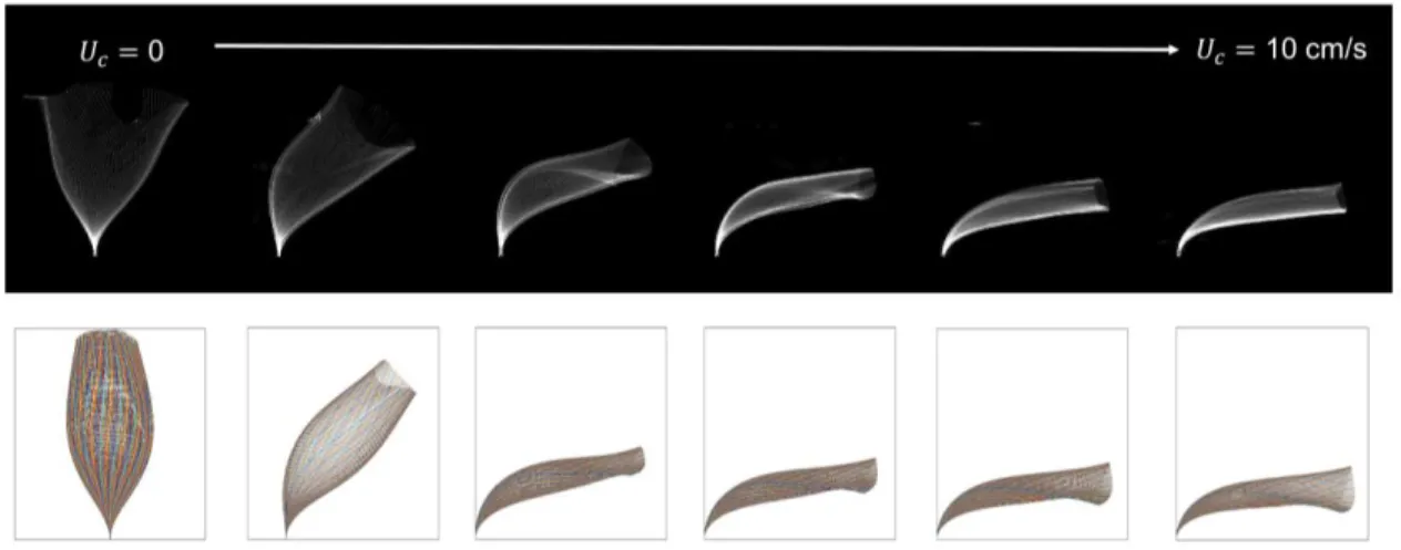
Figure 5. Schematic of the force balance in eqn. (28). 443 444 445 5. Results/Discussion 446 5.1. Blade imaging 447
Figure 6 shows the motion of an individual blade over one wave period, comparing 448
digital images and simulated motion. The wave condition was held constant across 449
scenarios (𝑇 = 2 s, 𝑈𝑤 = 7.8 cm/s), and the current increased in six increments between 450
𝑈𝑐 = 0 and 10 cm/s (left to right in figure). Blade motion in the zero-current case was 451
similar to that in the convective regime in Leclercq and de Langre (2018). In this regime, 452
the blade moved completely passively with the fluid particles over most of the blade 453
length and most of the wave cycle. As the current increased, the mean pronation of the 454
blade increased and the range of blade motion decreased. The simulated blade motion 455
was qualitatively similar to the observed motion (Fig. 6). 456
The mean deflected height, ℎ𝑑, was defined as the vertical distance between the 457
time-mean position of the blade tip and the bed. The mean deflected height decreased 458
with increasing current magnitude (Figure 7). Luhar and Nepf (2013) provide an 459
empirical equation for deflected height in unidirectional currents without waves (eqn. (4) 460
in Luhar and Nepf 2013, but repeated here). 461 ℎ𝑑 𝑙 = 1 − 1−𝐶𝑎−1/4 1+𝐶𝑎− 3 5(4+𝐵 3 5)+𝐶𝑎−2(8+𝐵2) (32) 462
This equation is plotted as a solid curve in Figure 7 using the current-only Cauchy 463
number i.e. 𝐶𝑎 = 𝐶𝑎𝑐 (eqn. (1)). The deflected height predicted from eqn. (32) agreed 464
with measured values within uncertainty. This indicated that the time-mean pronation 465
was dependent only on the time-mean velocity (current), even when the wave velocity 466
(𝑈𝑤 = 7.8 cm/s) was comparable to and even larger than the current velocity (𝑈𝑐 = 2 to 467
10 cm/s). Finally, the simulated values of ℎ𝑑 (squares in Figure 7) had reasonable 468
agreement with the measured values (circles in Figure 7), except for 𝐶𝑎𝑤𝑐 = 380 and 469
540, for which the simulation under-predicted the measured ℎ𝑑 by 21% and 24%, 470
respectively (Figure 7). 471
472
473
Figure 6. Blade motion over one wave cycle based on digital images of real blades (top row)
474
and numerical simulation (bottom row). For all images, 𝑙 = 10 cm, 𝑑 = 100 μm, 𝑇 = 2 s, 𝑈𝑤 = 475
7.8 cm/s, 𝐶𝑎𝑤= 252 and 𝐿 = 4.0. Current increased from left to right (0, 2.0, 4.0, 6.0, 8.0, 10.0 476
cm/s), with 0 ≤ 𝐶𝑎𝑐 ≤ 800. 477
478
Figure 7: Mean deflected height, ℎ𝑑, from digital images (circles) and numerical simulation 479
(squares). Black solid line denotes eqn. (32) evaluated using the current-only Cauchy number, 480
𝐶𝑎𝑐. Error bars indicate the 95% confidence interval for mean deflected height estimated from 5 481
individual wave cycles from the digital imaging. 482
483
5.2. Measured forces on model rigid and flexible blades. 484
The assumption that 𝐶𝐷,𝑤𝑐 = 𝐶𝐷,𝑤 was confirmed using measured forces on rigid 485
blades to estimate the drag coefficient in combined wave-current conditions. For 𝑈𝑤 = 486
7.8 cm/s, and across all current values, the measured 𝐶𝐷,𝑤𝑐 = 3.7 ± 0.7, which agreed 487
with the wave only value predicted from eqn. (26), 𝐶𝐷,𝑤 = 4.0. Similarly, for 𝑈𝑤 = 11.0 488
cm/s, the measured value 𝐶𝐷,𝑤𝑐 = 3.1 ± 0.6, agreed with the predicted value 𝐶𝐷,𝑤 = 3.6. 489
Further, the ratio of drag coefficient in combined wave-current to pure waves 𝐶𝐷,𝑤𝑐⁄𝐶𝐷,𝑤 490
= 0.93 ± 0.18 and 0.86 ± 0.17, for 𝑈𝑤 = 7.8 and 11 cm/s, respectively, agreed with 491
Chandler and Hinwood’s (1982) observation that for 0 ≤ 𝑈𝑐
𝑈𝑤 ≤ 1.2, the ratio 𝐶𝐷,𝑤𝑐⁄𝐶𝐷,𝑤 is 492
in the range 0.7 to 1.1. In conclusion, for rigid blades, the assumption 𝐶𝐷,𝑤𝑐 = 𝐶𝐷,𝑤 was 493
reasonable. 494
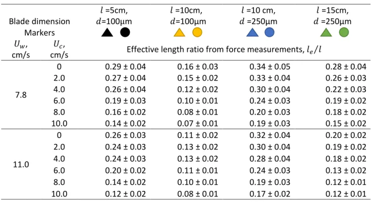
Based only on the measured forces on flexible and rigid blades, we calculated the 495
measured effective length ratio using eqn. (25), 𝑙𝑒⁄ (𝑚𝑒𝑎𝑠𝑢𝑟𝑒𝑑) =𝑙
𝐹𝑚𝑒𝑎𝑛 𝐹𝑚𝑒𝑎𝑛,𝑟𝑖𝑔𝑖𝑑. 496
Experimental results were shown in Table 1. In the supporting information (Figure S3), 497
we also compared the measured 𝑙𝑒⁄ with the simulated 𝑙𝑙 𝑒⁄ , which confirmed that the 𝑙 498
simulation recreated the measured values. 499
500
Table 1: Experimental values of 𝒍𝒆
𝒍 in combined wave-current conditions 502 Blade dimension 𝑙 =5cm, 𝑑=100μm 𝑙 =10cm, 𝑑=100μm 𝑙 =10 cm, 𝑑 =250μm 𝑙 =15cm, 𝑑 =250μm Markers 𝑈𝑤, cm/s 𝑈𝑐,
cm/s Effective length ratio from force measurements, 𝑙𝑒⁄ 𝑙
7.8 0 0.29 ± 0.04 0.16 ± 0.03 0.34 ± 0.05 0.28 ± 0.04 2.0 0.27 ± 0.04 0.15 ± 0.02 0.33 ± 0.04 0.26 ± 0.03 4.0 0.26 ± 0.04 0.12 ± 0.02 0.30 ± 0.04 0.22 ± 0.03 6.0 0.19 ± 0.03 0.10 ± 0.01 0.24 ± 0.03 0.19 ± 0.02 8.0 0.16 ± 0.02 0.08 ± 0.01 0.20 ± 0.03 0.18 ± 0.02 10.0 0.14 ± 0.02 0.07 ± 0.01 0.19 ± 0.03 0.15 ± 0.02 11.0 0 0.26 ± 0.03 0.11 ± 0.02 0.32 ± 0.04 0.20 ± 0.02 2.0 0.24 ± 0.03 0.13 ± 0.02 0.30 ± 0.04 0.19 ± 0.02 4.0 0.24 ± 0.03 0.13 ± 0.02 0.28 ± 0.04 0.18 ± 0.02 6.0 0.20 ± 0.02 0.11 ± 0.01 0.24 ± 0.03 0.13 ± 0.02 8.0 0.14 ± 0.02 0.10 ± 0.01 0.19 ± 0.03 0.12 ± 0.01 10.0 0.12 ± 0.02 0.08 ± 0.01 0.17 ± 0.02 0.12 ± 0.01 503 504
5.3. Effective blade length behavior for combined wave and current 505
Measured and simulated values of effective length were used together to test the 506
proposed wave-current model for effective blade length (eqn. (13)), as well as the 507
hypothesized thresholds for current-dominated (𝑈𝑐 > 2𝑈𝑤) and wave-dominated (𝑈𝑐 < 508
1
4𝑈𝑤) drag conditions. Figure 8 compares the measured (circles) and simulated 509
(crosses) effective blade lengths with the scaling equations shown with solid curves. 510
The four sub-plots represent different combinations of blade geometry (see figure 511
caption) and wave velocity (𝑈𝑤 = 11 cm/s and 7.8 cm/s). For each blade-wave 512
combination, the current velocity was varied from 𝑈𝑐 = 0 to 30 cm/s. Importantly, these 513
conditions all fall in the range of short waves, specifically, L > 1. For reference, the 514
proposed limits of 𝑈𝑐 = 1
4𝑈𝑤 and 𝑈𝑐 = 2𝑈𝑤 are indicated in Figure 8 with red vertical 515
lines. For 𝑈𝑐 < 1
4𝑈𝑤, the measured and simulated effective lengths converged with the 516
wave-only scaling (eqn. (9), shown with thin horizontal line in Figure 8), with deviations 517
of less than 15%. For 𝑈𝑐 > 2𝑈𝑤, 𝑙𝑒⁄ converged with the current-only scaling (eqn. (6), 𝑙 518
shown with thin black curve in Figure 8), with deviations less than 5%. These two 519
observations confirmed the limits defined in Section 2 for wave-dominated and current-520
dominated behavior. In between these limits, 𝑙𝑒⁄ had good agreement with the new 𝑙 521
wave-current formula, eqn. (13), shown with heavy black curve in Figure 8, with 522
deviations of less than 16%. Note, the current-dominated and combined wave-current 523
models converged when 𝑈𝑐⁄𝑈𝑤 > 2. Finally, the new, wave-current formula (eqn. (13), 524
heavy black curve in Figure 8) provided a reasonable prediction for all 𝑈𝑐⁄𝑈𝑤 values, 525
with a maximum deviation 20%, showing that the new predictor smoothly captures the 526
full range of current to wave ratios. 527
528
529
Figure 8. Effective blade length normalized by full blade length, 𝑙𝑒⁄ , versus velocity 𝑙 530
ratio, 𝑈𝑐⁄𝑈𝑤. Circles (o) denote measured values, and crosses (x) denote simulated values. 531
The proposed wave-current model described by eqn. (13) is shown with a heavy black curve 532
and labeled in sub-plot (a). The thin horizontal line denotes the wave-only scaling law, eqn. (9). 533
The thin black curve denotes the current-only scaling law, eqn. (6). The vertical red lines denote 534
the expected thresholds for wave-dominated (𝑈𝑐⁄𝑈𝑤< 1
4), and current-dominated (𝑈𝑐⁄𝑈𝑤> 2) 535
conditions. Blade geometry and wave conditions in each subplot: (a) 𝑙 = 10 cm, 𝑑 = 250 um, 536 𝑏 = 1 cm, 𝑈𝑤= 11 cm/s (b) 𝑙 = 10 cm, 𝑑 = 250 um, 𝑏 = 1 cm, 𝑈𝑤= 7.8 cm/s (c) 𝑙 = 10 cm, 𝑑 = 537 100 um, 𝑏 = 1 cm, 𝑈𝑤 = 11 cm/s (d) 𝑙 = 10 cm, 𝑑 = 100 um, 𝑏 = 1 cm, 𝑈𝑤= 7.8 cm/s. 538 539
5.4. Long waves without current, 𝑳 ≪ 𝟏 540
For long waves (large wave excursion 𝐴𝑤) or short blades (small 𝑙), the ratio of 541
blade length to wave excursion is small (𝐿 = 𝑙 𝐴⁄ 𝑤 ≪ 1), and the blade cannot follow the 542
fluid motion during the entire wave cycle. Instead, the blade remains pronated but 543
nearly stationary during a large fraction of the wave period. For simplicity, these were 544
called long-wave conditions. For long-wave conditions, we hypothesized that the 545
effective blade length could be described by the unidirectional current model (eqn. (6)), 546
using the equivalent mean velocity √1/2 𝑈𝑤. Specifically, we hypothesized that for 𝐿 << 547
1, 𝑙𝑒⁄ = 1.1𝐶𝑎𝑙 𝑤−1/3 (eqn. (10)). Because this wave condition was outside the operating 548
capabilities of the water channel, the proposed model was evaluated using the 549
simulation. The simulated blade length and thickness were 𝑙 = 10 cm and 𝑑 = 100 um, 550
respectively. The wave amplitude was 𝑎𝑤 = 1.5 cm, and the wave period was varied 551
from 𝑇 = 1 to 100s, yielding 𝐿 from 0.071 to 12, which spanned the long- and short-wave 552
regimes, 𝐿 << and >>1, respectively. The simulated effective blade lengths were 553
compared to the predicted effective blade length by considering the ratio of predicted 𝑙𝑒 554
to simulated 𝑙𝑒 (Figure 9). For triangles (∆), predicted 𝑙𝑒 was calculated from the 555
hypothesized long-wave equation (eqn. (10)). For crosses (x), predicted 𝑙𝑒 was 556
calculated from the short-wave equation (eqn. (9)). Figure 9 shows that for 𝐿 < 1 (long 557
waves, or short blades), the long-wave equation (triangles, eqn. (10)) gave a more 558
accurate prediction of 𝑙𝑒, i.e. the ratio was close to 1 with a maximum deviation of 7%. 559
For 𝐿 > 1 (short waves or long blades), the short-wave equation (crosses, eqn. (9)) 560
gave a more accurate prediction of 𝑙𝑒, i.e. the ratio was close to 1 with a maximum 561
deviation of 15%. This comparison confirmed the hypothesized long-wave equation 562
(eqn. (10)) for 𝐿 < 1. Between 𝐿 = 1 and 5, both equations did well, and for 𝐿 > 5 only 563
the short-wave equation (eqn. (9)) provided a good prediction. 564
565
Figure 9: Ratio of the effective blade length predicted from the two pure-wave scaling 566
laws to the simulated effective blade length versus the blade length ratio 𝐿 = 𝑙 𝐴⁄ 𝑤. For 567
triangle (∆) symbols the long-wave equation (eqn. (10)) was used to predict the effective 568
blade length. For cross (x) the short-wave equation (eqn. (9)) was used to predict the 569
effective blade length. The vertical dotted line denotes the threshold 𝐿 = 1. 570
571 572
Summary 573
Luhar and Nepf (2011, 2016) previously defined the effective blade length, 𝑙𝑒, to 574
characterize the impact of reconfiguration on the drag force experienced by an individual 575
blade in unidirectional flow and in waves. The effective length is defined as the length of 576
a rigid blade that experiences the same drag as a flexible blade of length 𝑙. This study 577
proposed a new equation to predict the effective blade length in combined wave-current 578
conditions. The new equation was confirmed using forces measured on flexible and rigid 579
blades. In addition, a numerical model that simulated blade motion and forces on a flexible 580
blade was validated using digital images of blade motion and the measured forces. Once 581
validated, the numerical model was used to explore a wider parameter space than was 582
available with the experimental facility. For a fixed wave condition, increasing current 583
magnitude decreased both the mean deflected height and the range of blade motion. The 584
mean deflected height had good agreement with the empirical equation for uni-directional 585
current without waves (Luhar and Nepf, 2013), indicating that the presence of waves did 586
not significantly impact the mean deflected height. The effective blade length was shown 587
to be a function of both current and wave magnitude, and three regimes were identified 588
for conditions with short waves (𝐿 >1). For 𝑈𝑐 < 0.25 𝑈𝑤, the blade motion was wave-589
dominated and the effective blade length was predicted by wave-only scaling (eqn. 9). 590
For 𝑈𝑐 > 2𝑈𝑤, the blade motion was current dominated, and the effective blade length 591
was predicted from the current-only scaling (eqn. (6)). In between these limits, 592
0.25 𝑈𝑤 < 𝑈𝑐 < 2𝑈𝑤, the effective blade length was predicted by the new wave-current 593
equation (eqn. (13)). Finally, the effective blade length for long waves, 𝐿 = 𝑙 𝐴⁄ 𝑤 < 1, was 594
shown to follow the scaling for pure current, but using the equivalent mean velocity √1/2 595 𝑈𝑤. 596 597 Acknowledgement 598
This material is based upon work supported by the National Science Foundation under 599
grant EAR 1659923. Any opinions, findings, and conclusions or recommendations 600
expressed in this material are those of the author(s) and do not necessarily reflect the 601
views of the National Science Foundation. Data and MATLAB code are included in the 602
PhD Thesis of Jiarui Lei, which will be available on MIT D-Space (https://dspace.mit.edu/), 603
or may be obtained from Jiarui Lei (email: [email protected]). 604
605
References 606
Alben, S., M. Shelley, and J. Zhang (2002). Drag reduction through self-similar bending
607
of a flexible body. Nature, 420(6915), 479, doi: 10.1038/nature01232.
Arkema, K., R. Griffin, S. Maldonado, J. Silver, J. Suckale, and A. Guerry (2017).
609
Linking social, ecological, and physical science to advance natural and nature‐
610
based protection for coastal communities. Annals of the New York Academy of
611
Sciences, doi: 10.1111/nyas.13322.
612
Augustin, L. N., J. L. Irish, and P. Lynett (2009). Laboratory and numerical studies of
613
wave damping by emergent and near-emergent wetland vegetation. Coastal
614
Engineering, 56(3), 332-340, doi: 10.1016/j.coastaleng.2008.09.004.
615
Barbier, E., S. Hacker, C. Kennedy, E. Koch, A. Stier, and B. Silliman (2011). The value
616
of estuarine and coastal ecosystem services. Ecological Monographs, 81(2),
169-617
193, doi: 10.1890/10-1510.1.
618
Bradley, K., and C. Houser (2009). Relative velocity of seagrass blades: Implications for
619
wave attenuation in low‐energy environments. JGR Earth Surface, 114(F1), doi:
620
10.1029/2007JF000951.
621
Chandler, B. D., and J. B. Hinwood (1982). Combined wave-current forces on horizontal
622
cylinders. In Coastal Engineering 1982 (pp. 2171-2188), doi:
623
10.1061/9780872623736.130.
624
Costanza, R., R. d'Arge, R. De Groot, S. Farber, M. Grasso, B. Hannon, K. Limburg, S.
625
Naeem, R. V. O'neill, J. Paruelo, and R. G. Raskin (1997). The value of the world's 626
ecosystem services and natural capital. Nature, 387(6630), 253-260, doi: 627
10.1038/387253a0. 628
Dalrymple, R., J. Kirby, and P. Hwang (1984). Wave diffraction due to areas of energy
629
dissipation. J. Water., Port, Coastal, Ocean Eng., 110(1): 67-79, doi:
630
10.1061/(ASCE)0733-950X(1984)110:1(67).
631
Ellington, C. P. (1991). Aerodynamics and the origin of insect flight. In Advances in
632
Insect Physiology (Vol. 23, pp. 171-210). Academic Press, doi:
10.1016/S0065-633
2806(08)60094-6.
634
Fornberg, B. (1998). Classroom note: Calculation of weights in finite difference
635
formulas. SIAM review, 40(3), 685-691.
636
Fourqurean, J. W., C. M. Duarte, H. Kennedy, N. Marbà, M. Holmer, M. A. Mateo, E. T.
637
Apostolaki, G. A. Kendrick, D. K. Jenson, K. J. McGlathery, and O. Serrano (2012).
638
Seagrass ecosystems as a globally significant carbon stock. Nature
639
geoscience, 5(7), 505, doi: 10.1038/ngeo1477.
640
Ghisalberti, M., and H. M. Nepf (2002), Mixing layers and coherent structures in
641
vegetated aquatic flows, J. Geophys. Res., 107(C2), 3011, doi:
642
10.1029/2001JC000871.
643
Goda, Y., & Suzuki, Y. (1977). Estimation of incident and reflected waves in random 644
wave experiments. In Coastal Engineering 1976 (pp. 828-845), doi: 645
10.1061/9780872620834.048. 646
Gosselin, F., E. de Langre, and B. A. Machado-Almeida (2010). Drag reduction of
647
flexible plates by reconfiguration. Journal of Fluid Mechanics, 650, 319-341, doi:
648
10.1017/S0022112009993673.
649
Houser, C., S. Trimble, and B. Morales (2015) Influence of blade flexibility on the drag
650
coefficient of aquatic vegetation. Estuaries and Coasts, 38(2):569-577, doi:
651
10.1007/s12237-014-9840-3.
Hu, Z., T. Suzuki, T. Zitman, W. Uittewaal, and M. Stive (2015). Laboratory study on
653
wave dissipation by vegetation in combined current–wave flow. Coastal
654
Engineering, 88, 131-142, doi: 10.1016/j.coastaleng.2014.02.009.
655
Infantes, E., A. Orfila, J. Terrados, M. Luhar, G. Simarro, and H. Nepf (2012) Effect of a 656
seagrass (Posidonia oceanica) meadow on wave propagation. Mar. Ecol. Prog. 657
Ser., 456:63-72, doi: 10.3354/meps09754.
658
Keulegan, G., and L. H. Carpenter (1958). Forces on cylinder and plates in an
659
oscillating fluid. J. Res. Nat. Bur. Stand., 60(5):423-440, doi: 10.6028/jres.060.043.
660
Leclercq, T., and E. de Langre (2018). Reconfiguration of elastic blades in oscillatory
661
flow. J. Fluid Mech., 838:606-630, doi:10.1017/jfm.2017.910
662
Lei, J., and H. Nepf (2016). Impact of current speed on mass flux to a model flexible
663
seagrass blade. Journal of Geophysical Research: Oceans, 121(7), 4763-4776, doi:
664
10.1002/2016JC011826.
665
Lei, J., and H. Nepf (2019). Wave damping by flexible vegetation: connecting individual 666
blade dynamics to the meadow scale. Coastal Engineering, accepted. 667
Li, C. W., and K. Yan (2007). Numerical investigation of wave–current–vegetation
668
interaction. Journal of Hydraulic Engineering, 133(7), 794-803, doi:
669
10.1061/(ASCE)0733-9429(2007)133:7(794).
670
Losada, I. J., M. Maza and J. L. Lara (2016). A new formulation for vegetation-induced
671
damping under combined waves and currents. Coastal Engineering, 107, 1-13, doi:
672
10.1016/j.coastaleng.2015.09.011.
673
Luhar, M., and H. Nepf (2011) Flow induced reconfiguration of buoyant and flexible 674
aquatic vegetation. Limnol. Ocean., 56(6):2003-2017, 675
doi:10.4319/lo.2011.56.6.2003.
676
Luhar, M. and H. Nepf (2016) Wave-induced dynamics of flexible blades. J. Fluids & 677
Structures, 61:20-41, doi.org/10.1016/j.jfluidstructs.2015.11.007.
678
Luhar, M., E. Infantes, and H. Nepf (2017) Seagrass blade motion under waves and its 679
impact on wave decay. JGR-Oceans, 122, doi:10.1002/2017JC012731.
680
Luhar, M. (2012). Analytical and experimental studies of plant-flow interaction at
681
multiple scales (Doctoral dissertation, Massachusetts Institute of Technology).
682
Luhar, M., and H. M. Nepf (2013). From the blade scale to the reach scale: A
683
characterization of aquatic vegetative drag. Advances in Water Resources, 51,
305-684
316, doi: 10.1016/j.advwatres.2012.02.002.
685
Mendez, F. J., and I. J. Losada (2004). An empirical model to estimate the propagation
686
of random breaking and nonbreaking waves over vegetation fields. Coastal
687
Engineering, 51(2), 103-118, doi:10.1016/j.coastaleng.2003.11.003.
688
Mullarney, J. and S. Henderson (2010). Wave‐forced motion of submerged single‐stem
689
vegetation. JGR- Oceans, 115(C12), doi: 10.1029/2010JC006448.
690
Paul, M., and C. L. Amos (2011). Spatial and seasonal variation in wave attenuation
691
over Zostera noltii. Journal of Geophysical Research: Oceans, 116(C8), doi:
692
10.1029/2010JC006797.
693
Paul, M., T. J. Bouma, and C. L. Amos (2012). Wave attenuation by submerged
694
vegetation: combining the effect of organism traits and tidal current. Marine Ecology
695
Progress Series, 444, 31-41, doi: 10.3354/meps09489.
Stratigaki, V., E. Manca, P. Prinos, I. J. Losada, J. L. Lara, M. Sclavo, C. L. Amos, I.
697
Caceres, and A. Sánchez-Arcilla (2011). Large-scale experiments on wave
698
propagation over Posidonia oceanica. Journal of Hydraulic Research, 49(sup1),
31-699
43, doi: 10.1080/00221686.2011.583388.
700
Taylor, J. 1997. An Introduction to Error Analysis: The Study of Uncertainties in
701
Physical Measurements. 2nd Ed., Oxford University Press.
702
Waycott, M., B. J. Longstaff, and J. Mellors (2005). Seagrass population dynamics and
703
water quality in the Great Barrier Reef region: a review and future research
704
directions. Marine Pollution Bulletin, 51(1-4), 343-350, doi:
705
10.1016/j.marpolbul.2005.01.017.
706
Ysebaert, T., S. L. Yang, L. Zhang, Q. He, T. J. Bouma, and P. M. Herman (2011).
707
Wave attenuation by two contrasting ecosystem engineering salt marsh
708
macrophytes in the intertidal pioneer zone. Wetlands, 31(6), 1043-1054, doi:
709
10.1007/s13157-011-0240-1.
710
Zeller, R., J. Weitzman, M. Abbett, F. Zarama O. Fringer, and J. Koseff (2014).
711
Improved parameterization of seagrass blade dynamics and wave attenuation
712
based on numerical and laboratory experiments. Limnol. and Ocean., 59(1),
251-713
266, doi: 10.4319/lo.2014.59.1.0251.
714 715