Automatic detection of periodic sources in the K2 data sets

Automatic Detection of Periodic Sources in the K2

Data Sets

by

Momchil Emil Molnar

Submitted to the Department of Physics

in partial fulfillment of the requirements for the degree of

Bachelor of Science

at the

MASSACHUSETTS INSTITUTE OF TECHNOLOGY

SACHUSETTS INSTITUTE OF TECHNOLOGY

JUL

07

2016

LIBRARIES

ARCHIVES

June 2016

@

Momchil Emil Molnar, MMXVI. All rights reserved.

The author hereby grants to MIT permission to reproduce and to

distribute publicly paper and electronic copies of this thesis document

in whole or in part in any medium now known or hereafter created.

Signature redacted

...-Department of Physics

May 17, 2016

C ertified by ...

Signature redacted

Saul A. Rappaport

Professor of Physics, Emeritus

Thesis Supervisor

Accepted by

...

Signature redacted

Professor Nergis Mavalvala

Senior Thesis Coordinator, Department of Physics

Automatic Detection of Periodic Sources in the K2 Data Sets

by

Momchil Emil Molnar

Submitted to the Department of Physics on May 17, 2016, in partial fulfillment of the

requirements for the degree of Bachelor of Science

Abstract

We present an automated algorithm for the detection of periodic sources in the K2 data sets. Fast discreet Fourier transformations are used to compute the Fourier spectra of the targets and two different detection algorithms for identifying signifi-cant signals are used. The first technique searches through the DFT to identify peaks that are significantly above the background noise level, and which have at least one higher harmonic of the fundamental frequency. We show this approach to be rela-tively inefficient for detecting weaker sources with narrow features, such as transiting exoplanets. The second algorithm that we apply uses a summation of the DFT har-monics, which relies on the fact that typical planetary transits and binary eclipses have numerous harmonics in their Fourier spectra. In this method we sum the har-monics of the fundamental frequency, which increases the signal-to-noise ratio and substantially increases the detection efficiency of the algorithm. This latter technique yields a smaller number of false positives while having higher detection rates than the first approach. A discussion of the noise level and detection threshold is presented, with a derivation of the threshold for the algorithm based on the noise properties in the K2 data. Furthermore, a discussion of the performance of both algorithms is presented. We then apply this automated search algorithm to the sixth and seventh fields of the K2 mission. In all these fields contained some 45,000 stars that were monitored for nearly three months each. The automated search yielded about 2000 interesting periodic targets. We conclude with a short discussion of the more inter-esting objects detected in the C7 data release by the K2 team. Finally, we present a catalog of many of the periodic sources that we have detected using these algorithms in the Appendix.

Thesis Supervisor: Saul A. Rappaport Title: Professor of Physics, Emeritus

Acknowledgments

The author wants to express his deepest gratitude to Prof. Saul Rappaport for his patient guidance and excellent advice, which lead to the completion of this thesis. Furthermore, we would like to thank Dr. Alan Levine and Prof. Belinda Kalomeni for the useful discussions and comments about the efficiency of the code. We would like to express our thankfulness for the confirmation of detected objects by Fei Dai. Finally, the author feels obliged to appreciate the help from Rumen Hristov for the useful optimization suggestions for the code.

Contents

1 Introduction 15

1.1 The Kepler Mission ... 15

1.1.1 K 2 m ission . . . . 16

1.2 Observed Objects in the K2 mission . . . . 18

1.2.1 Binary Stars . . . . 19

1.2.2 Pulsating Stars . . . . 23

1.2.3 Exoplanets . . . . 27

2 Using Fourier Transformations for finding periodic sources 29 2.0.1 Introduction to Discreet Fast Fourier Transformations . . . . . 30

2.0.2 "Zero padding" . . . . 30

2.1 Preprocessing of the K2 data . . . . 32

2.1.1 Boxcar filtering . . . . 32

2.2 Detection algorithms . . . . 36

2.2.1 Excluding the imprint of the thrusters . . . . 36

2.2.2 Detecting Harmonic Peaks in the FT Spectrum . . . . 36

2.2.3 Summation of Harmonic Peaks - Better SNR . . . . 37

2.2.4 Determining the detection threshold . . . . 39 3 Results from using the code

3.0.1 Folding of the data . . . .

3.1 Results from using the Harmonics Detection Method . . . .

3.2 Results from the summation of Harmonic Peaks . . . .

43 43 44 45 7

3.2.1 Double-Period folding . . . . 4 Data Analysis and Further Work on K2 observational Campaign 7 47

4.1 Planet Candidates . . . .

4.2 Interesting Binary Stars ...

A The Convolution theorem and the Fourier transform of the Boxcar filter

47 49

53 B Detected Planet Candidates

C Detected Binary Stars D Detected Pulsating Stars

8

List of Figures

1-1 External view of the Kepler telescope. Source: Wikipedia . . . . 17

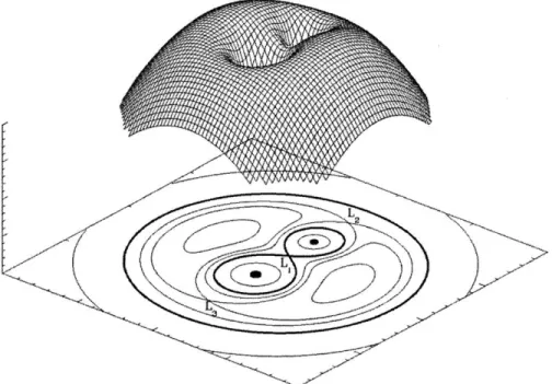
1-2 Schematic of the Kepler instruments of the telescope. Source: Wikipedia 17 1-3 The gravitational-inertial potential of a binary system in the co-rotating

reference frame. The potential is projected as equipotential lines on the plane below. The drop-like bold shape around the two stars (the black dots) are the Roche Lobes of the two stars. L1, L2, L3 are the

first three Lagrange points of the system. Source: Wikipedia . . . . . 20

1-4 The detached binary with EPIC number 21338208 observed during the C7 observational campaign of the K2 mission. Note the primary and

the secondary eclipses. . . . . 21

1-5 The binary star of type W Uma with EPIC number 21338208 observed during the C7 observational campaign of the K2 mission. The period

of the system is 0.37 days. . . . . 22

1-6 HR diagram with superimposed regions where different types of pulsat-ing stars are found. The region on the HR diagram where the pulsatpulsat-ing stars (J-Scuti stars, RR Lyrae stars, W Vir stars, 6-Cepheids, RV Tau stars) are found is named the "instability" strip, because most stars in

this region exhibit pulsations. Source: Chandra Web-page . . . . 24

1-7 Lightcurve of the RR-Lyrae type star EPIC 213705835 with period of 0.68 days. The variations of the lightcurve are due to the variability of

the amplitude of pulsations, known as Blazhko effect. . . . . 26

1-8 The lightcurve of the planet EPIC 217671466 with period of 1.92 days. This planet was confirmed from ground-based obserbervations before

being monitored with K2. . . . . 27

2-1 Illustration of the concepts presented in subsection 2.0.2. The example signal is s(t) = sin 10t + sin 10.6t. It was sampled 300 times in the range {0, 47r} and is presented in Fig. 2-la. The signal in 2-la was zero-padded up to 10' samples and the result is shown in Fig.2-1b. Fig. 2-1c presents the DFT of the signal in 2-la, while Fig.2-1d is the DFT

of the signal in Fig.2-1b. . . . . 31

2-2 Example of how a boxcar filter alters the signal of EPIC 204043888. The filter excludes all long-period contributions to the signal, but makes the FFT components in the range of days or less more

obvi-ous. . . . . 34

2-3 Transmissivity of the applied boxcar filter with moving average of AT = 1 day as the blue curve. The green curve shows the shape

of the sinc (wAT) function. . . . . 35

2-4 The probability distribution of the amplitude of the noise in the Fourier transformation of the K2 data (red dots). The black curve shows a fit of the probability distribution of white noise. Apparently, the noise in the K2 data deviates from the notion of white noise, which requires

numerical calculating its properties. . . . . 41

4-1 Object EPIC 213926179 which is an eclipsing binary with irregular

eclipse shapes. . . . . 50

4-2 Object EPIC 215825200 is an eclipsing binary in the center of a

plan-etary nebula. One of the components of the binary is a white dwarfs. 50

4-3 Object EPIC 213926179 which is an sdB eclipsing binary showing two

eclipses and a strong irradiation curve. . . . . 51

List of Tables

2.1 _{Table of the harmonics of the thrusters' fundamental frequency (fo)}

and their multiplicity . . . . 37

4.1 Table of the detected planet candidates and confirmed planets in the

C7 field with the harmonic summation method. HAT is a survey for detection of exoplanets lead by Princeton. These results were cross-checked with Fei Dei, a graduate student in the Kavli Institute for

Astrophysics and Space Research. . . . . 49

B.1 Set 1 (of 2) Detected Planet Candidates . . . . B.2 Set 2 (of 2) Detected Planet Candidates . . . . C.1 Set 1 (of 25) Detected Binary Stars . . . . C.2 Set 2 (of 25) Detected Binary Stars . . . . C.3 Set 3 (of 25) Detected Binary Stars . . . . C.4 Set 4 (of 25) Detected Binary Stars . . . . C.5 Set 5 (of 25) Detected Binary Stars . . . . C.6 Set 6 (of 25) Detected Binary Stars . . . . C.7 Set 7 (of 25) Detected Binary Stars . . . .. C.8 Set 8 (of 25) Detected Binary Stars . . . . C.9 Set 9 (of 25) Detected Binary Stars . . . . C.10 Set 10 (of 25) Detected Binary Stars . . . .. . . . C.11 Set 11 (of 25) Detected Binary Stars . . . .

C.12 Set 12 (of 25) Detected Binary Stars . . . . 11

C.13 Set 13 (of 25) Detected Binary Stars C.14 Set 14 (of 25) Detected Binary Stars C.15 Set 15 (of 25) Detected Binary Stars C.16 Set 16 (of 25) Detected Binary Stars C.17 Set 17 (of 25) Detected Binary Stars C.18 Set 18 (of 25) Detected Binary Stars C.19 Set 19 (of 25) Detected Binary Stars C.20 Set 20 (of 25) Detected Binary Stars C.21 Set 21 (of 25) Detected Binary Stars C.22 Set 22 (of 25) Detected Binary Stars C.23 Set 23 (of 25) Detected Binary Stars C.24 Set 24 (of 25) Detected Binary Stars C.25 Set 25 (of 25) Detected Binary Stars D.1 Set 1 (of 25) Detected Pulsating Stars D.2 Set 2 (of 25) Detected Pulsating Stars D.3 Set 3 (of 25) Detected Pulsating Stars D.4 Set 4 (of 25) Detected Pulsating Stars D.5 Set 5 (of 25) Detected Pulsating Stars D.6 Set 6 (of 25) Detected Pulsating Stars D.7 Set 7 (of 25) Detected Pulsating Stars D.8 Set 8 (of 25) Detected Pulsating Stars D.9 Set 9 (of 25) Detected Pulsating Stars D.10 Set 10 (of 25) Detected Pulsating Stars D.11 Set 11 (of 25) Detected Pulsating Stars D.12 Set 12 (of 25) Detected Pulsating Stars D. 13 Set 13 (of 25) Detected Pulsating Stars D.14 Set 14 (of 25) Detected Pulsating Stars D.15 Set 15 (of 25) Detected Pulsating Stars D.16 Set 16 (of 25) Detected Pulsating Stars

D.17 Set 17 (of 25) Detected Pulsating Stars D.18 Set 18 (of 25) Detected Pulsating Stars D.19 Set 19 (of 25) Detected Pulsating Stars D.20 Set 20 (of 25) Detected Pulsating Stars D.21 Set 21 (of 25) Detected Pulsating Stars D.22 Set 22 (of 25) Detected Pulsating Stars D.23 Set 23 (of 25) Detected Pulsating Stars D.24 Set 24 (of 25) Detected Pulsating Stars D.25 Set 25 (of 25) Detected Pulsating Stars

Chapter 1

Introduction

In this thesis, we will present an automated scripted algorithm for the detection of periodic sources in the K2 data sets of the Kepler follow-on mission. This script is needed because the telescope observes about 20,000 objects for three months and then changes its field of view. The large number of observed objects would make the manual processing of each individual object a rather tedious task. The algorithm we

present picks out the - 5% of the stars that exhibit periodic phenomena. This is not

a trivial task even via manual processing, especially when it comes to low-signal-to-noise ratio objects, such as exoplanets.

The algorithm relies on basic numerical techniques (Fast Fourier transforms, har-monic summation, boxcar filtering), which makes it versatile and applicable to other similar missions, such as TESS, which will be launched in 2017.

The basic concepts which are used in the later chapters will be presented in the Introduction, as well as some details about the Kepler mission.

1.1

The Kepler Mission

Kepler is a space telescope launched by NASA in 2009 in an Earth trailing orbit. It was designed principally for detecting Earth-sized exoplanets in the habitable zones of their host stars through very precise photometric observations. The telescope observed 145,000 stars in its field of view nearly continuously for four years. Besides

discovering over 2,000 planets, Kepler contributed precision photometric observations of binary star systems, stellar oscillations, and the first observed supernova shockwave (KSN 2011d).

The telescope has a Schmidt design with a primary mirror of 1.4 meters and a correction plate with a diameter of 0.95 meters (see Fig. 1-2). The mission can

boast the biggest array of CCD cameras of any scientific mission in orbit - the actual

photometer in the Kepler mission consists of 42 CCDs with 2200x1400 pixels each. This enables the telescope to have a field of view of 115 deg2_{. The main goal of the}

mission was to observe many stars continuously over a period of years in a search for exoplanets. Therefore, the field of view was chosen near the Milky Way, where the concentration of stars is highest on the sky. [41

Since the monitored stars were relatively bright (between 10"-16"'), the CCDs were read out every six seconds and summed every 58.89 seconds (for short cadence objects) or every 1765.5 seconds (for long cadence objects). Furthermore, the mission used a soft focus for the optical system (of ~ 4"), in order to decrease the pixel-sensitivity related noise.

The accuracy goal for the photometry of the mission was 20 parts per million (ppm) for a 6.5 hour integration time for a V=12' star. This can be compared to an 85 ppm change for an Earth-like planet transiting across a Sun like star. The

acquired noise levels for solar type stars were 29 ppm, which is - 50% worse than

anticipated, which required an extension of the mission to reach the same goals.[6

1.1.1

K2 mission

The planned duration of the Kepler mission was 3.5 years, but in April 2012 it was extended until 2016. However, a failure of the third of the reaction wheels of the telescope in May 2012 somewhat disabled the pointing system of the telescope, which ended the primary mission.

Since the photometric ability of the telescope was still functioning properly, the mission engineers devised a method to point the telescope using only the two func-tioning reaction wheels and the light pressure from the Sun. The mission was called

RCS Thruster Module (1of4)-. ~ Star Tracker Spaceaaft Electronics Oes>loyable Cover

Figure 1-1: External view of the Kepler telescope. Source: Wikipedia Focal Plane: 42CCDs, Schmidt Corrector with 0.95 m dia aperture stop Focal Plane Eleotronies:

clock drivers and

analog to digital converters

Mounting Collet >100 4 Fine Guidance Sensors sq deq FOV

Figure 1-2: Schematic of the Kepler instruments of the telescope. Source: Wikipedia

K2 or "Second Light".

This pointing method requires the telescope to be pointed in the plane of the ecliptic in order to most efficiently use the torque of the light pressure from the Sun. Therefore, the observations are being conducted only in regions of the sky close to the ecliptic plane, with the thrusters correcting for the slight drift every 6 hours. Furthermore, the telescope has to switch its 'field of view every 85 days to avoid sunlight entering the optical system.

These limitations impose the schedule of the observational campaigns. Each

ob-servational campaign, denoted by capital C, lasts about 85 days. The continuous

observations last for approximately 75 days. The remaining 10 days are used for transferring the data back to Earth, realigning the telescope and performing calibra-tions of the photometric system. Usually, the processed data are publicly released two months after the end of each observational campaign.

Due to bandwidth limitations on the amount of data transferred to Earth, the K2 mission will observe a smaller number of objects than the primary mission. Each campaign will include -100 short cadence objects and - 25,000 long cadence objects.

The K2 campaign uses the Ecliptic Plane Input Catalog (EPIC) [51 for cata-loging the targets in the mission. In the' thesis all the discussed targets will be listed with their EPIC number, which can easily be related to other astronomical catalogs through the MAST website (URL: http://archive.stsci.edu/k2/data-search/ search.php).

1.2

Observed Objects in the K2 mission

The K2 mission observational list is completely community driven. The program accepts observational requests from both unaffiliated and U.S. affiliated observers.

Since the fields of view of K2 are predetermined, the observers are supposed to propose interesting objects lying in regions of the sky that will be observed along ecliptic. Previously observed objects for K2 include brown dwarfs, exoplanet candi-dates, Kuiper belt objects, binary stars, star clusters, active galaxies and many other

exotic astrophysical objects.

Since the topic of this thesis is about detecting periodical celestial sources, we are interested in studying the properties of the most common of them in the K2 data sets

- binary and pulsating stars, as well as exoplanet candidates.

1.2.1

Binary Stars

Most of the stars in the Universe are in binary or multiple systems. In these systems the components orbit around a common center of mass (CM) with typical periods

from ~10 minutes to 105 years. The vast range of the periods allows for very

dif-ferent properties of these systems, due to the greatly varying distance between the components.

The Kepler telescope measures only the brightness of the observed objects in a single waveband. The angular resolution of the instrument is not sufficient to spatially resolve the two (or more) components of the binary systems. Thus, we can observe only the binaries whose orbital plane lies close to our line of sight. This leads to photometric variations due to eclipses between the two components, or due to ellipsoidal light variations (ELV) caused by the mutual tidal distortion of the two stars. Photometric observations of eclipses and ELVs allow us to measure various properties of the binary systems including the orbital periods, stellar radii and the ratio of the two stellar masses. Therefore, these objects are a valuable source of very accurate information about the properties of the constituent stars, which is invaluable information for stellar modeling.

Roche lobe and Lagrange points

We will introduce several concepts which will be useful for the following discussion of the different types of binary systems.

The Roche lobe of a star is the critical equipotential surface in a frame that rotates with the binary. The shape of the Roche lobe for a typical binary system has a figure "8"-like shape, as illustrated in Fig. 1-3. The intersection point of the Roche lobes of

'IA N SA

2 kzg

/ >-*

4-.-Figure 1-3: The gravitational-inertial potential of a binary system in the co-rotating reference frame. The potential is projected as equipotential lines on the plane below. The drop-like bold shape around the two stars (the black dots) are the Roche Lobes of the two stars. L1, L2, L3 are the first three Lagrange points of the system. Source:

Wikipedia

the two stars is called the first Lagrange point point (L1). The L1 point is a saddle

point in the Roche potential, which makes it a key place where mass is transferred in binary systems.

When one of the components of the binary system fills its Roche Lobe, the over-flowing matter is no longer gravitationally attached to that star and mass transfer starts through L1. This mechanism is called Roche lobe overflow (RLO) and is

re-sponsible for many observed phenomena, including Algol systems, the evolution of milisecond radio pulsars, X-ray binaries, cataclvsnic variables, and many others.

If both components of the system fill their Roche lobes, they can form a common

envelope (CE) that surrounds both stars.

20 If I

Detached binary stars

When )oth stars are ulnderfilling their Roche lobes, the system is called a detached

binary. In these systems, there is no mass transfer (unless there are strong stellar

winds) and the two stars evolve separately, as single stars. Their periods range froi

days up to thousands of years.

These systems are the easiest to model, since the comnJponeint stars are

gravitation-ally distorted to a lesser extent compared to closer binaries. Usugravitation-ally their lightcurves

conisist of almost constant flux (sometimes there are ellipsoidal variations and star

spots) sections interrlpted )y two distinct eclipses. Ai illustrative light curve of a

detached binary is provided in Fig.1-4.

Signal from the object ktwo213338208-c07 Ilc.fits 2.0 1.5 -' 1.0 -0.5 -0.0 I 0.0 0.2 0.4 0.6 0.8 1.0 Phase

Figure 1-4: The detached binary with EPIC number 21338208 olserved during the

C7 observatioial camJpaign of the K2 mission. Note the primary and the secondary

eclipses.

Semidetached and Contact binary systems

A Semidetached binary star is a system where only oiie of the components has filled

its Roche lobe amid it may be transferring material to the other star. The accretion

imaterial usually forms am accretion disc. due to the conservation of angular

momnen-tum. The evolution of the systei calm be donminated by the accretion. which chaiges

the masses of the two components an( their evolution, accordingly. 21

A Contact binary star is a system where both components have filled their Roche

lobes. These components of these systems are so close that the stars might share the

outermost layers of their atmospheres.1.2.1.

In both detached and semidetached binaries the components of the system are not nearly spherical, as in the case of a highly detached binary. The complicated geoinetry

of these systems makes their modeling harder and more intricate. Numerical codes like

PHOEBE (https://sourceforge.net/projects/phoebe/) are used for niodelling these systems. PHOEBE creates a numerical model of the binary star, where each component is a mesh recreating the gravitational equipotential surface of the star. which contains the observed parameters (surface brightness temperature). The code takes into account the orbital dynamics of the system while trying to reproduce the eclipses or the observed ELV. Furthermore. PHOEBE includes more physical phenomiena like starspots., limb darkening, third light, reflection and heating of the stars as well as other effects. This complicated numerical code is a versatile tool for analyzing the high-precision photometry lightcurves coming from Kepler and K2.

An example lightcurve for a contact binary is given in Fig.1-5. The system has a connon atmosphere and is namned after the first observed star of this kind - the star

NV from the constellation Ursa Major (W UMa stars).

Signal from the object ktwo214609225-c07Ilc.fits

1.3-1.2 - 1.1c 1.0 -0.9 0.8 0.7 -0.0 0.2 0.4 0.6 0.8 1.0 Phase

Figure 1-5: The binary star of type X Uma with EPIC number 21338208 observed during the C7 observational campaign of the K2 mission. The period of the system is 0.37 days.

1.2.2

Pulsating Stars

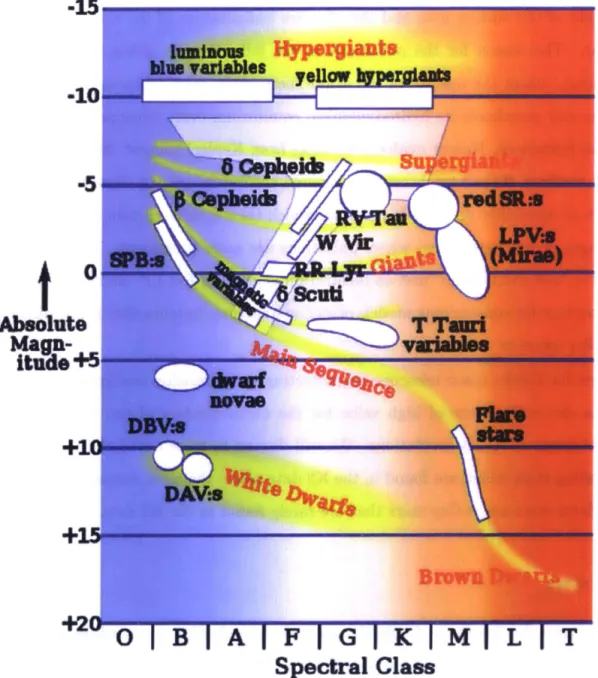
Pulsating stars are a type of variable stars, in which the luminosity changes due to variability of the surface area and the effective temperature of the surface layers of the star. The reason for the pulsations in the following discussion is the K-valve mechanism, where the opacity of the atmosphere varies with temperature in a way that the star overshoots its hydrodynamical equilibrium every cycle and this results in radial pulsations. Recent evidence (coming from Kepler) suggest that most types of stars oscillate, if their brightness is measured accurately enough. However, there is a region of instability on the HR diagram, which encompasses certain stellar masses and stages of their evolution, where pulsations are more prominent. This region is called the "instability strip" and an illustration is given in Fig.1-6. Stellar pulsations are important for constraining models of stellar structure, because they probe directly the stellar interiors.

Since the Kepler space telescope is conducting high-precision continuous photom-etry, its observations are of high value for the understanding of the nature of the different types of stellar oscillations. We will discuss in more detail the three types

of pulsating stars which are found in the K2 data sets - the most common RR Lyrae

and 6-Scuti stars and 6-Cep stars that are rarely found in the K2 data.

6-Cep stars

6-Cep stars, also known as Cepheids, are radially pulsating stars, whose radii and

temperatures vary with periods of tens of days. They are more massive than the Sun

- their masses range from 4 MD to 20 MO and are more luminous - up to 100,000 L®. Cepheids are Population 1 objects, which means that they are young, metal rich stars.

The pulsations of the Cepheids are driven by the K-mechanism, first described by

A. Eddington. The K stands for the change of opacity of the atmosphere of the stars.11

The driving principle is that doubly ionized helium is more opaque than singly ionized helium. Thus, at the start of each pulsation of a Cepheid, the star heats up, the singly

t

Absolute

Map-ltuile+s

+

A

F

G

K

M

Spectral Class

Figure 1-6: HR diagram with superimposed regions where different types of pulsating stars are found. The region on the HR diagram where the pulsating stars ( 5-Scuti stars, RR Lyrae stars, W Vir stars, 5-Cepheids, RV Tau stars) are found is named the "instability" strip, because most stars in this region exhibit pulsations. Source: Chandra Web-page

ionized helium loses one more electron and the atmosphere becomes optically thicker. The increased radiation pressure expands the star and cools it down, until the helium layer becomes singly ionized and transparent to the radiation. Then the excess heat is radiated away and the star shrinks again under the influence of gravitation, and the whole process repeats. The resulting lightcurves of the Cepheids are very similar to those of RR-Lyrae stars, an example of which is shown in Fig.1-7.

The Cepheids are very important in astrophysics, due to their well established period-luminosity relation, which makes them an excellent tool for measuring dis-tances. They are very luminous, which makes them suitable for determining distances

galaxies up to - 30 Mpc. [11] Many of the other extragalactic distance

measure-ments (Tully-Fisher relation, surface brightness of galaxies, supernovae) techniques have their zero-points calibrated with Cepheids observed in nearby galaxies.

RR Lyrae stars

The RR Lyrae stars are a type of pulsating star, which are very similar in their light variations to the Cepheids. However, they are less massive (- 1 M0) and less

luminous (- 40-50 LO). Furthermore, they are Population 2 stars, which are metal

poor. [3]

RR Lyrae stars also have a relation between their periods and their luminosity and they are more abundant than the Cepheids. This makes them a standard candle for measuring more nearby distances in the Milky Way and the Local Group. They are often found on the horizontal branch of the H-R diagrams in the globular clusters, which is used extensively for determining the properties of the star clusters.

Some RR Lyrae stars exhibit modulations of their oscillation amplitude or their period, called Blazhko effect. The phenomenon is not fully understood, but there are two hypothesis. The first one is that the magnetic and the rotation axis of the stars are misaligned which leads to modulation of the fundamental frequency of oscillation of the stars due to magnetic effects. The other hypothesis is that there are nonlinear couplings between higher order oscillations modes and the fundamental one. The Kepler telescope observed hundreds of RR Lyrae in its main field and several hundred

in each K2 data set. A curious fact is that the bright star RR Lyrae itself was in the field of the original Kepler mission.

Folded flux from object EPIC 213705835 around period 0.68 days

1.6-1.4 M1.2 1.0-0 L 0.8 x 0.6 -0.4 -0.0 0.2 0.4 0.6 0.8 1.0 Phase

Figure 1-7: Lightcurve of the RR-Lyrae type star EPIC 213705835 with period of 0.68 days. The variations of the lightcurve are due to the variability of the amplitude of pulsations, known as Blazhko effect.

6-Scuti type stars

6-Scuti type stars are short period (tens of minutes to about 12 hours) stars, oscillating both radially and non-radially in a superposition of a number of different normal

modes at the same time. They are stars larger than the Sun - they have masses between 1.5 - 3 MO and are of spectral classes A2-F8. These stars have smaller brightness amplitudes of about 6m = 0.6m. The mechanism for their pulsations is

the same as the one in the Cepheids -the K-valve, which is due to the different opacity of helium in different states.

The 6-Scuti type stars are very important astrophysical objects for several reasons.

First, they serve as standard candles as far as the small Magellanic cloud, as they are the most abundant type of pulsating stars in the Milky Way. Furthermore, they oscillate in many different modes at the same time, so the Kepler observations provide data for asteroseismological studies (the study of stellar pulsations).

26

1.2.3 Exoplanets

The notion of planets orbiting other stars has been discussed by many scientists and philosophers over the centuries. However, the first definite detection of a terrestrial mass object came in 1992, when two Earth sized objects were detected around the pulsar PSR-1257+12.12 Three years later (1995), the first exoplanet orbiting a main

sequence star was detected M. Mayor and D. Queloz.

[9]

two thousand planets have been discovered and more than four thousand planet candidates are awaiting confirmation.

The main mission of the Kepler telescope was to detect exoplanets through the transit method. In this initial goal the mission has been extremely successful by discovering more than a thousand planets and a few thousand planet candidates. The data from Kepler showed that there is statistically speaking at least one planet orbiting most stars in the Milky Way. Furthermore, 1 of 5 stars like the Sun may have an Earth-like planet in their habitable zone.[10]

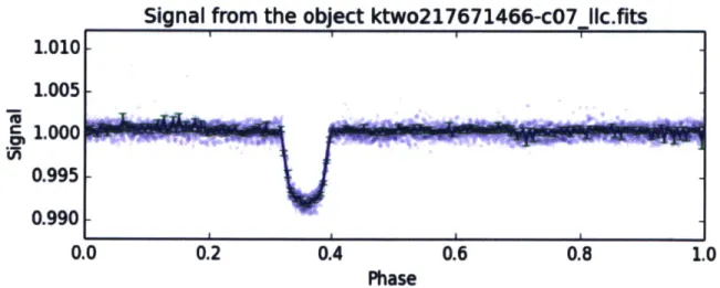
Signal from the object ktwo217671466-c07_Ilc.fits

1.010 1.005 ~1.ooo 0.995 0.990 L 0.0 0.2 0.4 0.6 0.8 1.0

Phase

Figure 1-8: The lightcurve of the planet EPIC 217671466 with period of 1.92 days. This planet was confirmed from ground-based obserbervations before being monitored with K2.

Even though the photometric precision of K2 is worse than the original Kepler mission (60 ppm vs 29 ppm), the data allow detection of exoplanet transits.17] Cur-rently, there are 46 confirmed planets and 270 planet candidates in the K2 campaigns (from C1 to C6). The number of discovered exoplanets is smaller than found in the

original Kepler mission, because the K2 observational campaigns are shorter (only 75 days) than the original Kepler observational campaign (several years). This in-troduces a detection bias toward short period systems, excluding the systems with periods greater than tens of days.

Chapter 2

Using Fourier

Transformations

for

finding periodic sources

In our search for periodic phenomena in the Kepler data (such as eclipses in binary systems or intrinsic stellar pulsations) we needed a method for detecting the peri-odic constituents of the observed flux. One well established method involves Fourier Transformations with some initial filtering of the raw data.

The approach to detecting statistically significant periodic signals is described in Ch.2.2. First, we will explain the details of Discreet Fourier transforms (DFT) in Section 2.0.1. Then the filtering and preprocessing of the raw data will be described in Sections 2.1.

Formally, a Fourier Transformation

f

f:

(w) = f(t)e-27r''dt (2.1)

This transformation

f is the signal f(t) represented in the frequency domain. The

magnitude of the complex function If(wo) is the relative strength of the w0 periodic

constituent of the signal. The functions spanning the spatial domain of the function

f

principle could be any set of orthogonal periodic functions. 29

2.0.1

Introduction to Discreet Fast Fourier Transformations

Since the observations by Kepler are taken at equal time intervals, we used the Dis-creet Fourier Transformations (DFT) algorithm.

The DFT takes a set of N evaluations of the function f(t) = f(kAt) at time

inter-vals At, where k = 0, 1, ... , N - 1. The result from the DFT is a discreet frequency

spectrum of the function f(t), which consists of the frequencies w" = N-t, where

n :0, 1, ... , N - 1. However, we will consider only the first half of the spectrum

-only the frequencies ranging from 0 to the Nyquist frequency (1). This constraint

is imposed, because the DFT cannot detect periodic signals above the Nyquist fre-quency.

In the case of Kepler, the telescope takes an image every 29.42 minutes. There-fore the sampling rate is 0.567 mHz and the highest frequency that can be detected (Nyquist frequency) is 0.2835 mHz or approximately ~ 1 hour. The lower bound on the frequency detection range is imposed from the length of the observational cam-paigns. For the K2 mission, one observational campaign is 78 days, which sets an upped limit for the detected periods to be approximately - 36 days.

The Fourier Transformations of the discreet signal was performed with the func-tion fft.fft in the numerical Python package NumPy. It utilizes the standard algo-rithm by Cooley and Tukey, published in 1965.[21 The set of algoalgo-rithms similar to the aforementioned are called Fast Fourier Transforms (FFT) because they reduce

significantly the complexity of the problem from O(n2_{) to O(n log n), by using the}

notion of sparse matrices, where n is the number of data samples to be transformed.

2.0.2

"Zero padding"

In order to improve the precision of the detected periods of the observed objects, we used a numerical technique called "zero padding". The basic idea behind this method is adding artificially a long sequence of zeros to the end of the data array. This action allows the DFT to achieve better frequency interpolation and thereby higher accuracy of the detected period. The higher resolution of the frequency spectra allows us to

2.0 2.0 1.5 1.0 0.5 0.0 -0.5 -1.0 -1.5 -2.0

(a) Input signal

300 samples. 1.0 0.5 0.0 -0.5 -1.0 -1.5 200 250 300 -2.0 s(t) = sin(10t) + sin(10.6t), 200 400 600 Bin number 800 1000

(b) The signal in 2-1a up to 103 samples.

/

8 9 10 11

Frequency, rei. Units

180 160 140 120 100 50 60 40 20

(c) DFT of the signal in 2-la.

7 8 9 10 11 12 13

Frequency, rel. units

(d) DFT of the signal in 2-1b.

Figure 2-1: Illustration of the concepts presented in subsection 2.0.2. The example signal is s(t) = sin 10t + sin 10.6t. It was sampled 300 times in the range {0, 4wr} and is presented in Fig. 2-la. The signal in 2-1a was zero-padded up to 10' samples and the result is shown in Fig.2-1b. Fig. 2-1c presents the DFT of the signal in 2-la, while Fig.2-1d is the DFT of the signal in Fig.2-1b.

31 4 4 4

I1~I~

L

!\

ri

measure the periods of the studied object with greater precision.

Through "zero padding", we effectively do not change the Fourier transformation of the signal, since the zero-valued bins do not contribute to the overlap integrals. How-ever, when we add N, zeros to a signal of N samples, the DFT returns (N+N2)/2+1 bins, which have the same information as the original N/2+1. The additional N, sam-ples give us higher apparent resolution, which enables us to measure the positions of the peaks more accurately.

2.1

Preprocessing of the K2 data

The data from the K2 mission are publicly available on the Mikulski Archive for Space Telescopes (MAST) (URL: https: //archive. stsci. edu/pub/k2/). The repository contains the FITS files for every EPIC target and its extracted lightcurves. In our work, we used the lightcurves provided by MAST, which are released approximately two months after the end of the observational campaign. These lightcurves required further corrections, since they have imperfect processing by the MAST pipeline. In the further subsections 2.2.1 and 2.1.1 we present the further filtering steps we take in order to improve the precision of the provided data.

2.1.1

Boxcar filtering

The presence of a significant amount of low-frequency noise in the data released by MAST necessitated utilizing a high-pass filter. We used a boxcar filtering (moving average of N bins), which was then subtracted from the initial data. This gave us an FT spectrum with lower noise levels coming from low frequencies. We chose to

average _{29 bins around each data measurement (which is about a day), as it allows}

us to detect variations with sinusoidal signals with P ,< 1 day and systems with sharp features in their lightcurves (e.g. transits or eclipses) up to P- 10 days.

The drawback of using this filter is that objects with longer period astrophysical variations will have attenuated FT amplitudes, because the peaks in their frequency spectrum will be affected by the filtering. Some long-period pulsating stars or binaries

with sinusoidal lightcurves would be most affected, but shorter duration phenomena such as exoplanet transits will not suffer significantly from the filtering. Thus, the fil-tering decreases the detection efficiency for low-frequency signals with periods greater than couple of days. However, the most interesting binaries, have periods on the order of days and sharp eclipses, which the filter will not adversely affect.

We can calculate analytically the transmissivity of the boxcar filter in the fre-quency domain.

Let's assume that we have an observed signal D(t) and a boxcar filter B(t), which is the moving mean over time period 2AT. The signal and the filter will have Fourier

transforms respectively b(w) and B(w), where w means frequency. We can show that,

B(w) = sinc (w) (see Appendix A). The filtered data, S(t) will be:

S(t) = D(t) - B(t) * D(t) (2.2)

where B(t) * D(t) is the convolution of the boxcar filter applied to the signal. If

we take the Fourier transform of equation 2.2 and use the convolution theorem (see Appendix A), we can show that:

S(w)

= b(w) (1 - sinc (wAT)) (2.4)

where we have removed the convolution of the filter ($) and the signal (b), due to the convolution theorem. Equation 2.4 shows us, that the transmissivity of the filter is described by the function T(w):

T(w) = 1 - sinc (wAT) (2.5)

The transmission of the filter in the frequency domain is illustrated in Fig.2-3. 33

Raw flux from the object EPIC 204043888 2070 2080 2090 2100 2110 2120 Time, days Raw FFT of EPIC 204043888 5 10 15 20 2130 2140 25 Frequency (day 1)

(a) Raw data and _{its FFT from EPIC 20404388. Note the thruster firings related peaks at}

4,8,16 days-].

Raw flux from the object EPIC 204043888

-T 2070 2080 2090 2100 2110 2120 Time, days Raw FFT of EPIC 204043888 -T 5 10 15 20 2130 2140 25 Frequency (day 1)

(b) Filtered data and its FFT from EPIC 204009278.

Figure 2-2: Example of how a boxcar filter alters the signal of EPIC 204043888. The filter excludes all long-period contributions to the signal. but makes the FFT coniponents in the range of days or less iore obvious.

34

I

[

-N

E

C

.2

Frequency

days-

Figure 2-3: Transmnissivity of the applied boxcar filter with moving average of AT 1 day as the blue curve. The green curve shows the shape of the sinc (wAT) function.

35

-- Transmission of the filter

-- Sinc(x) function

2.2

Detection algorithms

Having the computed DFT of the preprocessed data, as described in the previous sections (2.0.1 -2.1), the next step was the detection of the significant periodic signals. In this section we will discuss the two methods which were used, as well as some general caveats for optimizing the search algorithm. The results from using these methods are described in Chapter 3.

2.2.1

Excluding the imprint of the thrusters

In the Fourier spectra of weak sources, we observed peaks which appeared as harmon-ics and subharmonharmon-ics of a fundamental frequency of ~ 4.072 cycles/day. An example is provided in Fig.2-2. We concluded that these are residual effects on the corrected fluxes from the thruster firings of the satellite, which occur with the same frequency

(every 5.89 hours).

We compiled a table of the harmonic thruster firings frequencies and excluded the regions around these frequencies from the FT spectrum while searching for significant peaks. The variance of the positions of the thruster harmonic peaks was on the order of 10 frequency bins, therefore we excluded the region of 20 bins around the mean of every thruster peak. Compared to the width of a typical peak, which is on the order of hundreds of bins, we think that an insignificant number of targets will be missed due to this filtering.

In Table 2.1 we include some of the FT peaks associated with thruster firings, as well as which harmonic of the fundamental (5.9 hour) peak they are. Further-more, we observed three subharmonics at frequencies 1.02t0.005, 2.033 0.005 and 3.053+0.005, which correspond to multiplicity of 1/4, 1/2 and 3/4.

2.2.2

Detecting Harmonic Peaks in the FT Spectrum

If a periodic signal is observed, which does not have a similar shape to the gauge functions used, we expect the frequency spectra of this object to have harmonic peaks at multiples (2x,3x,4x) of the fundamental frequency. We can argue this from the

Peak frequency, days-, Multiplicity to fo

4.072 0.005 1

6.11 0.005 3/2

8.14 0.005 2

11.985 0.005 ~_ _ _3

Table 2.1: Table of the harmonics of the thrusters' fundamental frequency (fo) and their multiplicity.

fact that in order to construct the signal back from the gauge functions, we will need more than one gauge function. Therefore, we expect in the Fourier transformation of a periodic signal, which does not resemble a sinusoid, to exhibit harmonics of the fundamental frequency.

Using this notion, we added a script to the algorithm, which detects peaks in the frequency spectra and checks if they have harmonics. In order for the peak in the Fourier transform to be detected as significant, it has to have a magnitude above a certain detection threshold which will be discussed in subsection 2.2.4. If the peak is high enough, then the algorithm checks if there are significant peaks at half or twice this frequency, following the same criteria as for the first one. If there is one significant harmonic, then the algorithm calculates the fundamental frequency (by the difference in the frequencies) and folds the flux.

2.2.3

Summation of Harmonic Peaks

-

Better SNR

When a lightcurve has sharp or narrow features, its Fourier transformation has many peaks, multiples of the fundamental frequency of oscillation. The power of the signal is redistributed among all the harmonics, which reduces the over signal-to-noise ratio of the real signal. For this reason, the algorithm described in subsection 2.2.2 is not as efficient for targets with many harmonics as it is for targets with fewer harmonics. However, many of the interesting objects have sharp and narrow features, like eclipses and transits, which produce many harmonics.

Therefore, we utilized a technique called "harmonic summation", which is prefer-able for weak sources with many harmonics in their frequency spectra, such as

planets.

The technique "harmonic summation" involves summation the multiples of a given base frequency. The underlying motivation is that the summation of the harmonics of the fundamental frequency will improve the signal-to-noise ratio. While using this method, for every bin in the DFT with frequency fo we summed its 10 multiple fractions of 10 ( 1foA fo,...,fo,fo):

10

Asum(fo) = A

(

n=1 f

where A(f) is the amplitude of the DFT at frequency f and Asum is the summed amplitude.

The implementation of this method creates a new array with the same length as the original DFT of the signal, where the frequency bins with the same positions will correspond to the same frequency. Then, the algorithm calculates the sum for each frequency fo and writes it in the new array. Finally, we apply the algorithm discussed in 2.2.2 to the summed spectra to look for significant peaks.

However, there might be more than one peak in the frequency spectrum that meets the detection criteria, because some of the harmonics of the fundamental frequency also attains high signal-to-noise ratio from the harmonic summation. Therefore, the script performs a global (over the whole frequency spectrum) search and detects the peak with the highest amplitude from all detected peaks.

Because, by construction, the detected peak has frequency ten times the

funda-mental, the actual frequency of the system is - of the detected frequency.₁₀

This method has a drawback for short period objects. The 1 0th harmonic of

the fundamental frequency might be above the Nyquist frequency, which leads to obtaining the wrong period for the object. This is observed for objects with periods of half a day or less, where the script folds the data around twice the correct period. This happens, because the peak corresponding to the fundamental frequency is above the Nyquist limit.

2.2.4

Determining the detection threshold

Determining the detection threshold is important for the efficiency of the algorithm. If the detection threshold is too low, then many false positive results will be detected. By contrast, if the detection threshold is too high, the weaker source will not be detected.

An empirical approach to estimate the detection threshold is to vary it while keeping track of how many real objects and how many false positives were detected. However, this method is not favored, because it requires a lot of computational time and the results might not be conclusive.

Therefore, we chose to determine the detection threshold based on the proper-ties of the noise in the Fourier transformations of previously published K2 data. First, we calculated the probability distribution of the amplitudes of the noise in the Fourier spectrum of three objects. The three objects used for the analysis were EPIC 212292753, EPIC 212292753 and EPIC 212293036 from the C6 campaign. They were chosen because they did not exhibit any periodic signatures in their lightcurves.

We calculated the probability distribution of the amplitudes of the noise in the Fourier transformations by computing a normalized distribution of the Fourier ampli-tudes over a small range of frequencies for the three sources. The frequency windows for which we collected the Fourier amplitudes were small compared to the full range of the frequency spectra, in order to avoid any frequency dependencies of the noise

properties. The result for the frequency window from 1.25 x 10-4 Hz to 2.083 x

10-Hz obtained from the three objects is presented in Fig.2-4.

The measured probability distribution of the noise amplitudes in the Fourier spec-tra of K2 data is presented as the red dots in Fig.2-4. We can see that it deviates from the probability distribution for white noise, graphed as the solid black line.

The white noise distribution is obtained by a two-parameter fit of the theoretical prediction for such type of noise:

P(a) = Alae-2/ A2 (2.7)

where a is the amplitude of the noise, A1 and A2 are free parameters. The best fit

was obtained for values of A1 =1911 22 and A2=0.02405 0.000144.

Similar results to Fig.2-4 were obtained for two other frequency ranges - from

0.694 x 10-4 Hz to 0.781 x 10-4 and from 0.972 x 104 Hz to 1.38 x 10-4 Hz. This

shows that the noise in the K2 data is not white and we have to calculate its properties numerically.

Our detection threshold is based on the local RMS and the mean of the frequency spectrum of the signal. We chose the mean and the RMS, because they are convenient measures of the local noise, which we can describe in a quantifiable manner from the results presented in Fig.2-4. Furthermore, from the probability distribution of the noise amplitudes we can numerically find what is the probability p(ao) for detecting a single noise amplitude above a threshold ao. For each target in the K2 data set we compute and inspect about 1500 independent frequency amplitudes. If we want a false alarm probability in a given source of -0.001, then the probability of a false

alarm per frequency component inspected should be - 1 x 10-6. We can numerically

integrate the probability distribution of the noise to obtain the threshold in terms of RMS and mean of the distribution that yields this probability.

The detection threshold calculated in this manner for the regular Fourier trans-form is equal to the mean of the frequency spectrum plus 4.54 times the RMS of the distribution. This detection threshold depends only on the local quantities

de-scribing the Fourier transformation - its mean and RMS. Therefore, for a peak to be

detected as significant, its amplitude has to be greater than the moving mean of the spectrum plus 4.54 times the moving RMS of the frequency spectra. We utilize the same threshold for the whole frequency domain, since we found very similar noise probability distributions for different parts of the frequency domain.

The locality of the measurements of the mean and the RMS is emphasized, since these two properties of the frequency spectrum change with frequency. However, we know that the probability distribution of the noise is similar for different frequencies. Therefore, we can estimate the local threshold based on its moving properties in different frequency ranges. In the implementation of the algorithm we calculated the

iiean and the average of the frequency spectrum over 500 bins. or over 1 100 of the whole spectrum. 60 50 L/n 40

CL)

Amplitude of the noise

Figure 2-4: The probability distribution of the amplitude of the noise in the Fourier transformation of the 12 data (red dots). The black curve shows a fit of the proba-bility (listribution of white noise. Apparently. the noise in the K2 data deviates from

the notion of white noise, which requires numerical calculating its properties.

The aforementioned threshold discussion is relevant for the method of detection

of harmonic peaks (subsection 2.2.2. but not for the Summed Harmonics technique

(subsection 2.2.3), because the properties of the noise in this case are different. There-fore. we repeated the same steps described above and the detection threshold for the

harmonic summation method is equal to the moving mean plus 3.42 times the moving

RMS of the local frequency spectrum.

Based on these detection criteria, we proceeded to use the algorithm. and the results are described in the next chapter. Since we utilized detectioni thresholds of

3.5 times and 4.5 tines the local R1MS of the frequency spectra for both the regular

FT search and the sumnned FT searches ._{we have shown them in Fig.2-4 as the cyai}

and magenta dotted lines.

41

Chapter 3

Results from using the code

We utilized both detection techniques discussed in section 2.2 and applied them to the available data sets (C1-C7). We were able to process the currently available data from campaigns 5, 6 and 7, which were released while I worked on this project. The results for C7, the last one released, are of the highest quality, after my optimization during the previous two campaigns (C5 and C6). The results from this campaign will be presented in Ch.4.

The code is implemented using Python and NumPy numerical library, which has precompiled functions with speed comparable to C/C++. Each check of an object takes approximately 6 seconds on a single core of an Intel i-7 3.4 GHz processor. If the code is run in parallel on 3 cores, it takes approximately 13 hours to go through the whole data set of about 25,000 objects.

3.0.1

Folding of the data

The raw lightcurves from the K2 mission are 70 days long and they are not very infor-mative by themselves, because their length makes it difficult to notice weak shorter time scale properties of the observed object. Therefore, all results are presented as lightcurves of "folded" fluxes about the fundamental period of each target.

Folding was carried out in the following way: first, the algorithm determines the fundamental frequency (and corresponding period) of the object. Then, for each data

point at time ti, the phase 41 was calculated in the following way:

4 mod (ti, Pfundamental) _(3.1)

Pfundamental

where mod(p,q) is the modulus of q from p and ti is the time of the observation. Afterwards, the phase interval [0,1] was divided into 250 equal intervals and the data

points were allocated according to their phase. Then, the average and the standard

deviation for each phase bin was calculated. On all plots presented in this thesis, the average for each bin is shown as the solid blue line, while the standard deviation

for each bin is marked with a green error bar. The error bars are not always visible, because the precision of the observations are often high compared to the amplitude of

some objects. The raw data are illustrated as the transparent blue dots on the plots.

3.1

Results from using the Harmonics Detection Method

The first method which we used for automatic detection was the Harmonic peak

detection, described in Chapter 2.2.2. It was implemented first, as it is required for.

the Harmonics summation method.

Based on the considerations about the threshold from the previous chapter, we

used a detection threshold of 4.5 RMS. The yield from this method was about 800

potential targets, which exhibit periodic behavior. There were about 350 (2%) false

positive detections, which was factor of 2 away from our goal of 1% false positives.

Thus, this detection method requires a higher signal-to-noise ratio threshold, which

would unfortunately also eliminate many of the weaker legitimate periodic targets

such as planet candidates.

Thus, we decided to lower the detection threshold down to 3.5 RMS of the fre-quency spectra. In this case, the number of detected astrophysical signals was about

1,200, but we found also about 3,500 false positives, which is unacceptable for this

project. Furthermore, this threshold was still too high for some of the exoplanetary candidates to be detected. Therefore, this detection method was not the best choice

for an automated detection of periodic objects.

3.2

Results from the summation of Harmonic Peaks

Using the implementation of the harmonics detection, mentioned in section 3.1, we utilized the harmonics summation technique, with a detection threshold of 3.5 RMS, as determined in Chapter 2. This technique yielded 1,858 detections of periodic sources from the C7 data set, with about 80 (3%) false positives. Since the results from this method are better, in terms of number of detected targets, at the same rate of false positives, we used the data set produced by this method for further analysis. The higher yield could be explained by the fact that the frequency spectrum of most interesting objects have multiple harmonics, which when are summed increase the signal-to-noise ratio of the object. Therefore, this method is more suitable for de-tecting systems with many harmonics; like exoplanets and binaries. The signals from pulsators like 6-Scuti and RR Lyrae stars are not enhanced with this algorithm, since they do not have that many harmonics, but usually their amplitudes are sufficiently big, that they're detected by either algorithm.

The only drawback of this algorithm is that it calculates 10 times the fundamental frequency. Sometimes, this might be above the Nyquist limit and, if detected at all, the fold will not be about the correct period.

3.2.1

Double-Period folding

Sometimes the harmonics of the fundamental frequency have an amplitude larger than the peak at the fundamental frequency. Then, the algorithm folds about an incorrect peak, and correspondingly about an incorrect period. Usually, the wrong harmonic which is detected is half the fundamental frequency, and we can then see two full periods of the system in the fold. However, in systems with multiple periods, like 6-Scuti type stars, this might yield a result which looks at first incorrect.