Publisher’s version / Version de l'éditeur:
Proceedings of the IEEE International Workshop on Machine Learning for Signal
Processing, 2009., 2009-09-04
READ THESE TERMS AND CONDITIONS CAREFULLY BEFORE USING THIS WEBSITE.
https://nrc-publications.canada.ca/eng/copyright
Vous avez des questions? Nous pouvons vous aider. Pour communiquer directement avec un auteur, consultez la
première page de la revue dans laquelle son article a été publié afin de trouver ses coordonnées. Si vous n’arrivez pas à les repérer, communiquez avec nous à [email protected].
Questions? Contact the NRC Publications Archive team at
[email protected]. If you wish to email the authors directly, please see the first page of the publication for their contact information.
NRC Publications Archive
Archives des publications du CNRC
This publication could be one of several versions: author’s original, accepted manuscript or the publisher’s version. / La version de cette publication peut être l’une des suivantes : la version prépublication de l’auteur, la version acceptée du manuscrit ou la version de l’éditeur.
Access and use of this website and the material on it are subject to the Terms and Conditions set forth at
Temporal Analysis of Text Data Using Latent Variable Models
Mølgaard, Lasse L.; Larsen, Jan; Goutte, Cyril
https://publications-cnrc.canada.ca/fra/droits
L’accès à ce site Web et l’utilisation de son contenu sont assujettis aux conditions présentées dans le site LISEZ CES CONDITIONS ATTENTIVEMENT AVANT D’UTILISER CE SITE WEB.
NRC Publications Record / Notice d'Archives des publications de CNRC:
https://nrc-publications.canada.ca/eng/view/object/?id=f04453f8-8bfb-4b25-9bf6-a576cf2cb400 https://publications-cnrc.canada.ca/fra/voir/objet/?id=f04453f8-8bfb-4b25-9bf6-a576cf2cb400TEMPORAL ANALYSIS OF TEXT DATA USING LATENT VARIABLE MODELS
Lasse L. Mølgaard
∗, Jan Larsen
Section for Cognitive Systems
DTU Informatics
DK-2800 Kgs. Lyngby, Denmark
{llm, jl}@imm.dtu.dk
Cyril Goutte
Interactive Language Technologies
National Research Council of Canada
Gatineau, Canada, QC J8X 3X7
[email protected]
ABSTRACT
Detecting and tracking of temporal data is an important task in multiple applications. In this paper we study temporal text mining methods for Music Information Retrieval. We compare two ways of detecting the temporal latent se-mantics of a corpus extracted from Wikipedia, using a stepwise Probabilistic Latent Semantic Analysis (PLSA) approach and a global multi-way PLSA method. The analysis indicates that the global analysis method is able to identify relevant trends which are difficult to get using a step-by-step approach. Furthermore we show that inspection of PLSA models with different number of factors may reveal the stability of temporal clusters making it possible to choose the relevant number of factors.
1. INTRODUCTION
Music Information Retrieval (MIR) is a multifaceted field, which until recently mostly focused on audio analysis. The use of textual descriptions, beyond using genres, has grown in popularity with the advent of different music websites, e.g. ”Myspace.com”, where abundant data about music has become easily available. This has for instance been inves-tigated in [1], where textual descriptions of music were re-trieved from the Web to find similarity of artists. The un-structured data retrieved using web crawling produces a lot of data, which requires cleaning to produce terms that ac-tually describe musical artists and concepts. Community-based music web services such as tagging Community-based systems, e.g. Last.fm, have also shown to be a good basis for ex-tracting latent semantics of musical track descriptions [2]. Despite these initial efforts it is still an open question how textual data is best used in MIR. The text-based methods have so far only considered text data without any structured
∗First author performed the work while visiting NRC Interactive
Lan-guage Technologies group.
knowledge. In this study we investigate if the incorporation of time information in latent factor models enhances the de-tection and description of topics.
Tensor methods in the context of text mining have re-cently received some attention using higher-order decom-position methods such as the PARAllel FACtors model [3] that can be seen as a generalization of Singular Value De-composition in higher dimensional arrays. The article [3] applies tensor decomposition methods successfully for topic detection in e-mail correspondence over a 12 month period. The article also employs a non-negatively constrained PA-RAFAC model forming a Nonnegative Tensor Factorization analogous to the well-known Nonnegative Matrix Factor-ization (NMF) [4].
Probabilistic Latent Semantic Analysis (PLSA) [5] and NMF have successfully been applied in many text analysis tasks to find interpretable latent factors. The two methods have been shown to be equivalent [6], where PLSA has the advantage of providing a direct probabilistic interpretation of the latent factors. Our work therefore investigates the extension of PLSA to tensors.
2. TEMPORAL TOPIC DETECTION
Detecting latent factors or topics in text using NMF and PLSA has assumed an unstructured and static collection of documents.
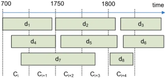
Extracting topics from a temporally changing text col-lection has received some attention lately, for instance by [7] and also touched by [8]. These works investigate text streams that contain documents that can be assigned a times-tamp y. The timestimes-tamp may for instance be the time a news story was released, or in the case of articles describ-ing artists it can be a timespan indicatdescrib-ing the active years of the artist. Finding the evolution of topics over time re-quires assigning documents d1, d2, ..., dmin the collection to time intervals y1, y2, ..., yl, as illustrated in figure 1. In contrast to the temporal topic detection approach in [7], we can assign documents to multiple time intervals, e.g. if the
d1 d4 d2 d5 d7 d6 time d3 d8 1700 1750 1800
Ci Ci+1 Ci+2 Ci+3 Ci+4
Fig. 1. An example of assigning a collection of documents di based on the time intervals the documents belong to. The assignment produces a document collection Ckfor each time interval
active years of an artist spans more than one of the chosen time intervals. The assignment of documents then provides lsub-collections C1, C2, ..., Clof documents.
The next step is to extract topics and track their evolu-tion over time.
2.1. Stepwise temporal PLSA
The approaches to temporal topic detection presented in [7] and [8] employ latent factor methods to extract distinct top-ics for each time interval, and then compare the found toptop-ics at succeeding time intervals to link the topics over time to form temporal topics.
We extract topics from each sub-collection Ck using a PLSA-model [5]. The model assumes that documents are represented as a bags-of-words where each document di is represented by an n-dimensional vector of counts of the terms in the vocabulary, forming an n×m term by document matrix for each sub-collection Ck. PLSA is defined as a la-tent topic model, where documents and terms are assumed independent conditionally over topics z:
P(t, d)k= Z X
z
P(t|z)kP(d|z)kP(z)k (1) This model can be estimated using the Expectation Maxi-mization (EM) algorithm, cf. [5].
The topic model found for each document sub-collection Ckwith parameters, θk = {P (t|z)k, P(d|z)k, P(z)k}, need to be stringed together with the model for the next time span θk+1. The comparison of topics is done by comparing the term profiles P(t|z)kfor the topics found in the PLSA model. The similarity of two profiles is naturally measured using the KL-divergence,
D(θk+1||θk) =X t
p(t|z)k+1logp(t|z)k+1 p(t|z)k . (2) Determining whether a topic is continued in the next time span is quite simply chosen based on a threshold λ, such that
two topics are linked if D(θk+1||θk) is smaller than a fixed threshold λ. In this case the asymmetric KL-divergence is used in accordance with [7]. The choice of the threshold must be tuned to find the temporal links that are relevant. 2.2. Multiway PLSA
The method presented above is useful to some extent, but does not fully utilize the time information that is contained in the data. Some approaches have used the temporal as-pect more directly, e.g. [9] where an incrementally trainable NMF-model is used to detect topics. This approach does in-clude some of the temporal knowledge but still lacks global view of the important topics viewed over the whole corpus of texts.
Using multiway models, also called tensor methods we can model the topics directly over time. The 2-way PLSA model in 1 can be extended to a 3-way model by also con-ditioning the topics over years y, as follows:
P(t, d, y) =X z
P(t|z)P (d|z)P (y|z)P (z) (3) The model parameters are estimated using maximum likeli-hood using the EM-algorithm, e.g. as in [10]. The expecta-tion step evaluates P(z|t, d, y) using the estimated parame-ters at step t.
(E-step): P(z|t, d, y) =P p(t|z)p(d|z)p(y|z)p(z) z′p(t|z
′)p(d|z′)p(y|z′)p(z′) (4) The M-step then updates the parameter estimates.
(M-step): P(z) =1 N X tdy xtdyP(z|t, d, y) (5) P(t|z) = P dyxtdyP(z|t, d, y) P tdyxtdyP(z|t, d, y) (6) P(d|z) = P tyxtdyP(z|t, d, y) P tdyxtdyP(z|t, d, y) (7) P(y|z) = P tdxtdyP(z|t, d, y) P tdyxtdyP(z|t, d, y) (8) The EM algorithm is guaranteed to converge to a local maximum of the likelihood. The EM algorithm is sensitive to initial conditions, so a number of methods to stabilize the estimation have been devised, e.g. Deterministic Annealing [5]. We have not employed these but instead rely on restart-ing the trainrestart-ing procedure a number of times to find a good solution.
The time complexity of the two PLSA approaches of course depends on the number of iterations for the method to converge. Basically the most expensive operation is the
E-step of the algorithms. The cost of each iteration for 2-way PLSA isO(RZ) which is calculated for each of the K time steps. R is the number of non-zeros in the term-doc matrix. Each iteration for multiway PLSA (mwPLSA), takesO(RZK) as all time-steps are calculated simultane-ously. In our experiments the algorithms typically converge in 40-50 iterations. However, the 2-way PLSA does have the advantage that the individual time steps can be calcu-lated in parallel giving a speed-up proportional to K. 2.3. Topic model interpretation
The latent factors z of the model can be seen as topics that are present in the data. The parameters of each topic can be used as descriptions of the topic. P(t|z) represents the probabilities of the terms for the topic z, thus providing a way to find words that are representative of the topic. The most straightforward method to find these keywords is to use the words with the highest probability P(t|z). This ap-proach unfortunately is somewhat flawed as the histogram reflects the overall frequency of words, which means that generally common words tend to dominate the P(t|z).
This effect can be neutralized by measuring the rele-vance of words in a topic relative to the probability in the other topics. Measuring the difference between the his-tograms for each topic can be measured by use of the sym-metrized Kullback-Leibler divergence:
KL(z, ¬z) =X t (P (t|z) − P (t|¬z)) log P(t|z) P(t|¬z) | {z } (9) wt
This quantity is a sum of contributions from each term t, wt. The terms that contribute with a large value of wtare those that are relatively more special for the topic z. wt can thus be used to choose the keywords. The keywords should be chosen from the terms that have a positive value of P(t|z) − P (t|¬z) and with the largest wt.
3. WIKIPEDIA DATA
In this experiment we investigated the description of com-posers in Wikipedia. This should provide us with a dataset that spans a number of years, and provides a wide range of topics. We performed the analysis on the Wikipedia data dump saved 27th of July 2008, retrieving all documents that Wikipedians assigned to composer categories such as ”Baroque composers” and ”American composers”. This produced a collection of 7358 documents, that were parsed so that only the running text was kept.
Initial investigations in music information web mining showed that artist names can heavily bias the results. There-fore words occurring in titles of documents, such as Wolf-gang Amadeus Mozart, are removed from the text corpus,
1600 1700 1800 1900 2000
0 1000 2000 3000
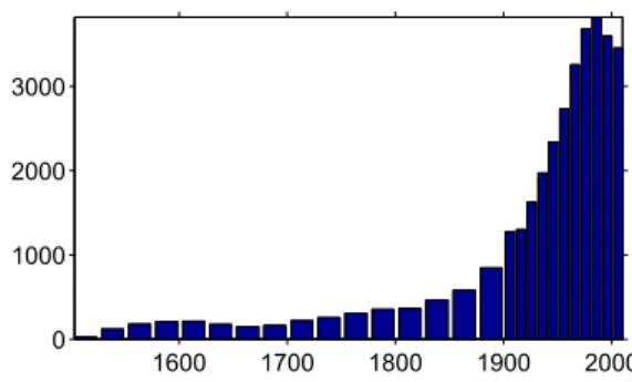
Fig. 2. Number of composer documents assigned to each of the chosen time spans.
i.e. occurrences of the terms ’wolfgang’, ’amadeus’, and ’mozart’ were removed from all documents in the corpus. Furthermore we removed irrelevant stopwords based on a list of 551 words. Finally terms that occurred fewer than 3 times counted over the whole dataset and terms not occur-ring in at least 3 different documents were removed.
The document collection was then represented using a bag-of-words representation forming a term-document ma-trix X where each element xtdrepresents the count of term t in document d. The vector xd thus represents the term histogram for document d.
To place the documents temporally the documents were parsed to find the birth and death dates. These data are sup-plied in Wikipedia as documents are assigned to categories such as ”1928 births” and ”2007 deaths”. The dataset con-tains active composers from around 1500 until today. The next step was then to choose the time spans to use. Inspec-tion of the data revealed that the number of composers be-fore 1900 is quite limited so the artists were assigned to time intervals of 25 years, giving a first time interval of [1501-1525]. After 1900 the time intervals were set to 10 years, for instance [1901-1910]. Composers were assigned to time intervals if they were alive in some of the years. We es-timated the years composers were active by removing the first 20 years of their lifetime. The resulting distribution of documents on the resulting 27 time intervals is seen in figure 2.
The term by document matrix was extended with the time information by assigning the term-vector for each com-poser document to each era, thus forming a 3-way tensor containing terms × documents × years. The tensor was further normalized over years, such that the weight of the document summed over years is the same as in the initial term doc-matrix. I.e. P(d) =Pt,yXtdy =
P
tXtd. This was done to avoid long-lived composers dominating the re-sulting topics.
The resulting tensor X ∈ Rm×n×lcontains 18536 terms x 7358 documents x 27 time slots with 4,038,752 non-zero entries (0.11% non-zero entries).
Canada, electronic symphony eurov ision popular music film, tv, theatre university opera
Symphony, opera, ballet russian 2000 1950 1900 church music 1875 1850
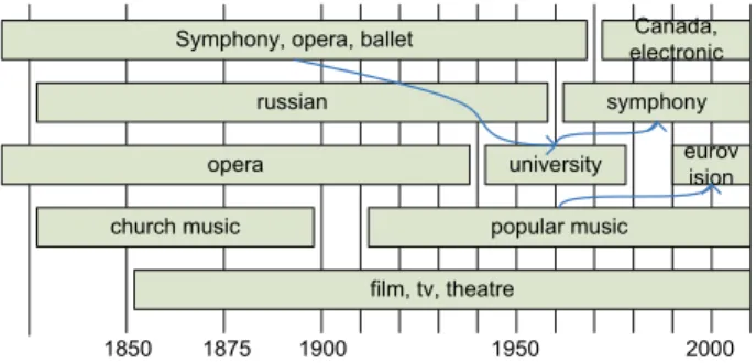
Fig. 3. Topics detected using step-by-step PLSA. The topics are depicted as connected boxes, but are the results of the KL-divergence-based linking between time slots
3.1. Term weighting
The performance of machine learning approaches in text mining often depends heavily on the preprocessing steps that are taken. Term weighting for LSA-like methods and NMF have thus shown to be paramount in getting inter-pretable results. We applied the well-known tf idf weight-ing scheme, usweight-ing tf = log(1 + xtdy) and the log-entropy document weighting, idf = 1 +PDd=1
htdlog htd logD , where htd= P yxtdy P
dyxtdy. The log local weighting minimizes the
ef-fect of very frequent words, while the entropy global weight tries to discriminate important terms from common ones. The documents in Wikipedia differ quite a lot in length, therefore we employ document normalization to avoid that long articles dominate the modeled topics.
4. EXPERIMENTS
We performed experiments on the Wikipedia composer data using the stepwise temporal PLSA method and the multiway-PLSA methods.
4.1. Stepwise temporal PLSA
The step-by-step method was trained with 5 and 16 topic PLSA models for each of the l sub-collections of documents described above. The PLSA models for each time span was trained using a stopping criterion of10−5relative change of the cost function, restarting the training 10 times for each model, choosing the model minimizing the likelihood. The two setups were chosen to have one model that extracts gen-eral topics and a model with a higher number of compo-nents that detects more specific topics. The temporal topics are produced by coupling the topics at time k and k+ 1 if the KL-divergence between the topic term distributions, D(θk+1|θk), is below a threshold λ. This choice of thresh-old produces a number of topics that stretch over several time spans. A low setting for λ may leave out important
re-lations, while a higher setting produces too many links to be interpretable. Figure 3 shows the topics found for the 20th century using the 5 component models. There are clearly 4 topics that are present throughout the whole period. The topics are film and TV music composers, which in the be-ginning contains Broadway/theater composers. The other dominant topic describes hit music composers. Quite inter-estingly this topic forks off a topic describing Eurovision song contest composers in the last decades.
Even though the descriptions of artists in Wikipedia con-tain a lot of bibliographical information it seems that the la-tent topics have musically meaningful keywords. As there was no use of a special vocabulary in the preprocessing phase, it is not obvious that these musically relevant phrases would be found.
The stepwise temporal PLSA approach has two basic shortcomings. The first is the difficulties in adjusting the threshold λ to find meaningful topics over time. The second is how to choose the number of components to use in the PLSA in each time span. The 5 topics that are used above do give some interpretable latent topics in the last decade as shown in figure 3. On the other hand the results for the ear-lier time spans (that contain less data), means that the PLSA model finds some quite specific topics at these time spans. As an example the period 1626-1650 has the following top-ics:
1626-1650
41% 34% 15% 8.7% 1.4% keyboard madrigal viol baroque anglican
organ baroque consort italy liturgi surviv motet lute poppea prayer italy continuo england italian respons church monodi charles lincoronazion durham nuremberg renaissance royalist opera english choral venetian masqu finta chiefli baroque style fretwork era england germani cappella charles’s venice church collect itali court teatro choral
The topics found here are quite meaningful in describing the baroque period, as the first topic describes the church music, and the second seems to find the musical styles, such as madrigals and motets. The last topic on the other hand only has a topic weight of P(z) = 1.4%. This tendency was even more distinct when using 16 components in each time span.
4.2. Multi-way PLSA
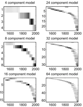
We then model the full tensor, described in section 3, using the mwPLSA model. Analogously with the stepwise tem-poral PLSA model we stopped training reaching a change of less than10−5 of the cost function. The main advan-tage of the mwPLSA method is that the temporal linking of topics is accomplished directly through the model estima-tion. The time evolution of topics can be visualized using the parameter P(y|z) that gives the weight of a component for each time span. Figure 4 shows the result for 4, 8, 16,
4 component model 1600 1800 2000 1 2 3 4 8 component model 1600 1800 2000 2 4 6 8 16 component model 1600 1800 2000 5 10 15 24 component model 1600 1800 2000 5 10 15 20 32 component model 1600 1800 2000 10 20 30 64 component model 1600 1800 2000 20 40 60
Fig. 4. Time view of components extracted using mwPLSA, showing the time profiles P(y|z) as a heatmap. A dark color corresponds to higher values of P(y|z)
32 and 64 components as a ”heatmap”, where darker colors correspond to higher values of P(y|z). The topics are gen-erally unimodally distributed over time so the model only finds topics that increase in relevance and then dies off with-out reappearing. The skewed distribution of documents over time which we described earlier emerges clearly in the dis-tribution of topics, as most of the topics are placed in the last century. Adding more topics to the model has two effects considering the plots. Firstly the topics seem to be sparser in time, finding topics that span fewer years. Using more topics decomposes the last century into more topics that must be semantically different as they almost all span the same years. Below we inspect the different topics to show how meaningful they are. The keywords extracted using the method mentioned above are shown in table 1, showing 5 of the topics extracted by the 32 component model, including the time spans that they belong to.
The first topic shown in table 1 is one of the two topics that accounts for the years 1626-1650, the keywords sum-marize the five topics found using mwPLSA. The second topic has the keywords ragtime and rag, placed in the years 1876-1921, which aligns remarkably well with the genre description on Wikipedia: ”Ragtime [...] is an originally American musical genre which enjoyed its peak popularity between 1897 and 1918.”1. The stepwise PLSA approach did also have ragtime as keywords in the 16 component
1http://en.wikipedia.org/wiki/Ragtime
1601-1700 1676-1776 1876-1921 1921-1981 1971-2008 2.10% 2.40% 4.70% 4.80% 6.40% baroque baroque ragtime concerto single italian opera sheet nazi chart church sonata rag war album continuo italian weltemignon symphony release survive court nunc piano hit
court harpsichord ysa ballet track organ italy schottisch neoclassical sold motet violinist dimitti neoclassic demo madrigal church blanch choir fan cathedral organ parri hochschul pop
Table 1. Keywords for 5 of 32 components in a mwPLSA model. The assignment of years is given from P(y|z) and percentages placed at each column are the corresponding component weights, P(z)
model, appearing as a topic from 1901-1920. The next topic seems to describe World War II, but also contains the neo-classical movement in neo-classical music. The 16 component stepwise temporal PLSA approach finds a number of top-ics from 1921-1940 that describe the war, such as a topic in 1921-1930 with keywords: war, time, year, life, influ-enceand two topics in 1931-1941, 1. time, war, year, life, styleand 2: theresienstadt, camp, auschwitz, deport, con-centration, nazi. These are quite unrelated to music, so it is evident that the global view of topics employed in the mwPLSA-model identifies neoclassicism to be the impor-tant keywords compared to topics from other time spans.
Some of the topics do overlap in time, such as the first two presented in table 1, and it is clear that they present different aspects of the music in the Baroque era, one repre-senting church music (organ and madrigals), while the other describes opera and sonatas. So the overlapping topics can show how genres evolve.
5. MULTI-RESOLUTION TOPICS
The use of different number of components in the mwPLSA model, as seen in figure 4, shows that the addition of topics to the model shrinks the number of years they span. The higher specificity of the topics when using more compo-nents gives a possibility to ”zoom” in on interesting topic, while the low complexity models can provide the long lines in the data.
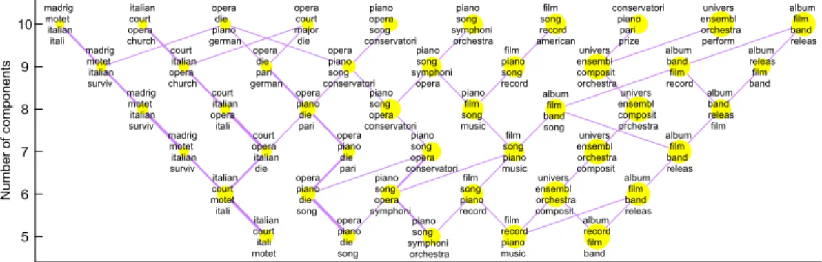
To illustrate how the clusters are related as we add top-ics to the model, we can generate a so-called clusterbush, as proposed in [11]. The result for the mwPLSA-based clus-tering is shown in figure 5. The clusters are sorted such that the clusters placed earliest in time are placed left. It is evident the clusters related to composers from the earlier centuries form small clusters that are very stable, while the later components are somewhat more ambiguous. The clus-terbush could therefore be good tool for exploring the topics at different timespans to get an estimate of the number of
5 6 7 8 9 10 Number of components italian court itali motet opera piano die song piano song symphoni orchestra film record piano music album record film band italian court motet itali opera piano die song piano song opera symphoni film song piano record univers ensembl orchestra composit album film band releas madrig motet italian surviv court opera italian die opera piano die pari piano song opera conservatori film song piano music univers ensembl orchestra composit album film band releas madrig motet italian surviv court italian opera itali opera piano die pari piano song opera conservatori piano film song music album film band song univers ensembl composit orchestra album band releas film madrig motet italian surviv court italian opera church opera die pari german opera piano song conservatori piano song symphoni opera film piano song record univers ensembl composit orchestra album band film record album releas film band madrig motet italian itali italian court opera church opera die piano german opera court major die piano opera song conservatori piano song symphoni orchestra film song record american conservatori piano pari prize univers ensembl orchestra perform album film band releas
Fig. 5. ”Cluster bush” visualisation of the results of the mwPLSA clustering of composers. The size of the circles correspond to the weight of the cluster, and the thickness of the line between circles how related the clusters are. Each cluster is represented by the keywords and is placed according to time from left to right.
components needed to describe the data. 6. CONCLUSION
We have investigated the use of time information in anal-ysis of musical text in Wikipedia. It was shown that the use of time information produces meaningful latent topics, which are not readily extractable from this text collection without any prior knowledge. The stepwise temporal PLSA approach is quite fast to train and processing for each time span can readily be processed in parallel. The model, how-ever, has the practical drawback that it requires a manual tuning of the linking threshold, and the lack of a global view of time in the training misses some topics. The multiway PLSA was shown to provide a more flexible and compact representation of the temporal data than stepwise temporal PLSA method. The flexible representation of the multiway model is a definite advantage, for instance when data has a skewed distribution as in the work resented here. The global model would also make it possible to do model selection over all time steps directly. The use of Wikipedia data also seems to be a very useful resource for semi-structured data for Music Information Retrieval that could be investigated further to harness the full potential of the data.
ACKNOWLEDGEMENTS
This work is supported by the Danish Technical Research Council, through the framework project ‘Intelligent Sound’, www.intelligentsound.org (STVF No. 26-04-0092).
7. REFERENCES
[1] P. Knees, E. Pampalk, and G. Widmer, “Artist classification with web-based data,” in Proceedings of ISMIR, Barcelona, Spain, 2004.
[2] M. Levy and M. Sandler, “Learning latent semantic models for music from social tags,” Journal of New Music Research, vol. 37, no. 2, pp. 137–150, 2008.
[3] B. Bader, M. Berry, and M. Browne, Survey of Text Mining II Clustering, Classification, and Retrieval, chapter Discus-sion tracking in Enron email using PARAFAC, pp. 147–163, Springer, 2008.
[4] D. D. Lee and H. S. Seung, “Learning the parts of objects by non-negative matrix factorization,” Nature, vol. 401, no. 6755, pp. 788–791, 1999.
[5] T. Hofmann, “Probabilistic Latent Semantic Indexing,” in Proc. 22nd Annual ACM Conf. on Research and Develop-ment in Information Retrieval, Berkeley, California, August 1999, pp. 50–57.
[6] E. Gaussier and C. Goutte, “Relation between plsa and nmf and implications,” in Proc. 28th annual ACM SIGIR
confer-ence, New York, NY, USA, 2005, pp. 601–602, ACM.
[7] Q. Mei and C. Zhai, “Discovering evolutionary theme pat-terns from text: an exploration of temporal text mining,” in Proc. of KDD 05. 2005, pp. 198–207, ACM Press.
[8] M. W. Berry and M. Brown, “Email surveillance using non-negative matrix factorization,” Computational and Mathe-matical Organization Theory, vol. 11, pp. 249–264, 2005. [9] B. Cao, D. Shen, J-T Sun, X. Wang, Q. Yang, and Z. Chen,
“Detect and track latent factors with online nonnegative ma-trix factorization,” in Proc. of IJCAI-07, Hyderabad, India, 2007, pp. 2689–2694.
[10] K. Yoshii, M. Goto, K. Komatani, T. Ogata, and H. G.
Okuno, “An efficient hybrid music recommender
sys-tem using an incrementally trainable probabilistic generative model,” Audio, Speech, and Language Processing, IEEE Transactions on, vol. 16, no. 2, pp. 435–447, Feb. 2008.
[11] F. ˚A. Nielsen, D. Balslev, and L. K. Hansen, “Mining the
pos-terior cingulate: Segregation between memory and pain com-ponents,” NeuroImage, vol. 27, no. 3, pp. 520–532, 2005.