HAL Id: hal-00704493
https://hal.archives-ouvertes.fr/hal-00704493
Submitted on 6 Jun 2012HAL is a multi-disciplinary open access archive for the deposit and dissemination of sci-entific research documents, whether they are pub-lished or not. The documents may come from teaching and research institutions in France or abroad, or from public or private research centers.
L’archive ouverte pluridisciplinaire HAL, est destinée au dépôt et à la diffusion de documents scientifiques de niveau recherche, publiés ou non, émanant des établissements d’enseignement et de recherche français ou étrangers, des laboratoires publics ou privés.
three-dimensional loading constraints
Christophe Duhamel, Philippe Lacomme, Hélène Toussaint
To cite this version:
Christophe Duhamel, Philippe Lacomme, Hélène Toussaint. A GRASP x ELS for the vehicle routing problem with three-dimensional loading constraints. 2011. �hal-00704493�
1
LIMOS, CNRS UMR 6158, Campus des Cézeaux, 63177 Aubière Cedex, France.
A GRASP
ELS for the vehicle routing
problem with three-dimensional
loading constraints
C. Duhamel
1, P. Lacomme
1, H. Toussaint
1Research Report LIMOS / RR-11-01
January 2011
2
A GRASP
ELS for the vehicle routing problem with
three-dimensional loading constraints
Christophe Duhamel, Philippe Lacomme
Hélène Toussaint
Laboratoire d'Informatique (LIMOS, UMR CNRS 6158), Campus des Cézeaux, 63177 Aubière Cedex, France.
Abstract
This paper addresses an extension of the Capacitated Vehicle Routing Problem where the client demand consists of three-dimensional weighted items (3L-CVRP). The objective is to design a set of trips for a homogenous fleet of vehicles based on a depot node which minimizes the total transportation cost. Items in each vehicle trip must satisfy the three-dimensional orthogonal packing constraints. A GRASP ELS algorithm is proposed to compute the best possible solution. We propose a new method to address the 3D packing which allows items to be rotated or not. It is based on a relaxation of the 3D problem in which items coordinates are first computed before getting compatible z-coordinates. Additional techniques are used to reduce as much as possible the time to check the 3D packing feasibility of trips. The effectiveness of our approach is evidenced through computational experiments on 3L-CVRP instances from the literature. New realistic instances are also proposed. These instances are based on the 96 French districts and encompass both small scale instances and large scale instances with up to 200 nodes
Keywords: Vehicle Routing, GRASP, Evolutionary local search, 3L-CVRP, 3D orthogonal packing
1
Introduction
1.1 Capacitated Vehicle Routing Problem and extensions with packing constraints
The Capacitated Vehicle Routing Problem (CVRP) is a classical NP-hard node routing problem which received a considerable amount of attention for decades [1] [2] [3]: it consists in optimally organizing vehicles trips in order to deliver goods required by a set of clients. It can be fully defined by considering a depot and a set of clients. Each one corresponds to a node of a complete graph where V is a set of n+1 nodes, 0 being the depot and nodes 1...n being the clients. Each edge has a finite cost and each node is given a demand . A fleet of homogeneous vehicles of limited capacity is located at the depot. The objective is to design a set of trips of minimal total cost to service all clients. A trip is a cycle performed by one vehicle. It starts at the depot, visits a subset of nodes, before returning to the depot. The trip total load is upper bounded by the vehicle capacity. Since split deliveries are not allowed, each client is serviced by exactly one vehicle. As stressed in [4], exact methods can only solve small to medium instance. Thus, medium and large CVRP instances are typically addressed by metaheuristics.
The 2L-CVRP is an extension of the CVRP which includes two-dimensional orthogonal rectangle loading constraints (the 2L constraints). This problem is essentially addressed in [5][6][7]. It can be reduced to the CVRP when the size of the items is not considered or when items are 1 1 squares, thus dealing only with their weight. The 2L-CVRP resolution has been first addressed by Iori et al. [8] using a branch and cut approach limited to small scale instances (less than 25 clients). Then Gendreau
et al. [5] introduced a tabu search algorithm. Zachariadis et al. [6] developed a guided tabu search.
Fuellerer et al. [7] proposed an efficient version of the Ant Colony scheme to solve the 2L-CVRP. Recently, Duhamel et al. [9] introduced a multi-start evolutionary local search scheme which outperforms all previous published methods. The approach is original as it does not address the 2L-CVRP during the main optimization process but rather a relaxation into the so-called RCPSP-2L-CVRP.
3
In the RCPSP-CVRP, the two-dimensional packing problem is relaxed into a RCPSP: at each point of the vehicle length the total width used must not exceed the vehicle width. Thus the vehicle width is related to the RCPSP resource availability. At the end of the main optimization process, the RSPCP-CVRP solution is transformed into a 2L-RSPCP-CVRP solution by a dedicated procedure. The authors showed in their experiments that most of the RCPSP-feasible solutions can be efficiently transformed into 2L-CVRP feasible solutions by only considering packing solutions which satisfy the previously computedx-abscissa.
The three-dimensional loading CVRP (3L-CVRP) is an extension of the 2L-CVRP where the height is also considered. More formally, each vehicle of the homogenous fleet is now defined by a weight capacity D and by a volume where is the vehicle length, is the vehicle width and is the vehicle height (related to (x, y, z) coordinates). The demand of each client consists of a set of items of total weight . Each item is a three-dimensional cuboid of length lik, width wik and height hik. Each client must be serviced by exactly one vehicle, which is
assigned to a single trip. A trip is a sequence of clients where corresponds to the depot. Each trip must be both “weight-feasible” and “packing-feasible”. A trip is “weight-feasible” if the total weight of carried items does not exceed the vehicle capacity, i.e. . It is “packing-feasible” if the client items can be loaded into the vehicle without overlapping and if it satisfies the classical orthogonal three-dimensional packing constraints. A set of “weight-feasible” and “packing-feasible” trips which involves all the clients defines a solution of the 3L-CVRP.
The 3L-CVRP has been addressed by Gendreau et al. [10] and more recently by Fuellerer et al. [11]. Only medium instances have been considered since three-dimensional packing problems are much harder to solve than their two-dimensional counterparts. The seminal publication of [10] introduces a tabu search algorithm that iteratively invokes a tabu search procedure for solving the inner loading sub-problem. Fuellerer et al. [11] introduce a highly efficient ant colony optimization algorithm which takes advantage of both fast packing heuristics for the loading sub-problem and of effective heuristics for the routing problem. These two publications also consider additional constraints about item fragility, LIFO unloading and support. Note that both instances from the literature and real-world instances were used by [10] to evaluate the performance of their method.
1.2 Cutting and Packing problems
1.2.1 General Cutting and Packing problems
Packing problems belong to the well-known family of cutting and packing problems. Many packing problems deal with the insertion of rectangular items in a rectangular bin in both two and three dimensions. They mostly differ on the objective function to optimize.
The Three-Dimensional Bin Packing Problem (3BPP) consists in packing a set of rectangular boxes into a minimal number of identical rectangular boxes [12] [13];
The Three-Dimensional Strip Packing Problem (3SPP) consists in packing a set of rectangular boxes into a strip of known width and infinite height so as to minimize the overall height of the packing [14] [15];
The Three-Dimensional Packing Problem (3PP) consists in checking if a set of rectangular boxes can be packed into one bin (rectangle box) of fixed size, see [16] for instance.
Several extensions have also been addressed over time, including but not limited to, rotation of items, limitations on the total weight and/or item costs.
4
The packing problem within the 3L-CVRP falls into the last category (3PP) since each trip has to be “packing-feasible”. A 3PP instance consists of a set of items which have to be packed into a bin of length , of width and of height . An item i has a length li , a width wiand a height hi ( .
A 3PP solution can be fully defined by the position of each item i, denoted (xi, yi, zi), into the bin. This
position corresponds to the coordinates of its bottom-left corner. Item rotation is only allowed in the (x, y) plane as rotations in other planes may be prohibited in the corresponding real-life application (items often have a "top" side for instance). Moreover the packing must be orthogonal, i.e. the items must be placed with their edges parallel to the sides of the bin.
Some authors have added extra constraints:
- fragility: the items tagged as “fragile” cannot be put under another item;
- support: each item must have a minimum “supporting area”, i.e. a given percent of its basis must be defined by the top of other items (or by the floor of the bin);
- LIFO: the items of any client in the trip can be unloaded by only using straight movements,
i.e. the items of a client i are not blocked by items of yet unvisited clients.
Such constraints correspond to realistic considerations in the industrial context of transportations and logistics. They are mandatory in many situations as CVRP solutions involving fully-loaded or nearly fully-loaded vehicles may not be 3L-CVRP feasible in practice, thus greatly reducing the interest of many CVRP commercial solvers.
2
GRASP
ELS framework for the 3L-CVRP
2.1 GRASP ELS Principle
The GRASP ELS [17] is a hybridization of the GRASP metaheuristic and of the ELS metaheuristic combining the positive features of both methods. The GRASP (Greedy Randomized Adaptive Search Procedure) [18] is a multi-start Local Search metaheuristic. At each iteration, an initial solution is constructed by using a greedy randomized heuristic. It is then improved by a local search and the best solution obtained at the end of each GRASP iteration is kept. The ELS (Evolutionary Local Search) [19] is an extension of the ILS (Iterated Local Search, [20]). At each iteration of the ELS, several copies of the current solution are done. Each copy is modified (mutation) before being improved by a Local Search. The best resulting solution is kept as the new current solution. The purpose of the ELS is to better investigate the neighbourhood of the current local optimum before leaving it, while the GRASP aims at managing the diversity during the solution space exploration. The framework we promote is a multi-start ELS in which the ELS is applied to the initial solutions generated by greedy randomized heuristics. Such an approach can also be viewed as a GRASP ELS in which the ELS is used as Local Search. Besides combining GRASP with ELS, another important feature of our approach is the alternation between two solution spaces: the giant tour space and the 3L-CVRP solution space. By defining genuine exploration on those two search spaces and by defining projections from one search space into the other one, one can more easily avoid being trapped in local optima. The high quality solutions obtained by Prins [19] for the VRP, alternating between two search spaces (giant tour and VRP solutions) is a clear illustration of approaches which manage alternation between a set of giant tours and a set of solutions.
Two solution representations are used: solutions encoded as giant tours (TSP tours on the n clients) and 3L-CVRP solutions encoded as the set of trips (see Figure 1). Converting a 3L-CVRP solution into a giant tour is done by the Concat procedure. It consists in removing the depot from each trip and then concatenating the resulting trips into a single one. The reverse operation, i.e. converting a giant tour into a 3L-CVRP, requires more work. It is usually done by a dedicated splitting procedure (Split) and it relies on dynamic programming. Such an approach has been successfully applied to numerous routing problems including the Capacitated Arc Routing Problem, the Vehicle Routing Problem, the Location Routing Problem for instance, see [21] for a recent state of the art of Split in routing
5
problems. As a giant trip is not a direct representation of a 3L-CVRP solution, we have chosen the inner ELS to work on 3L-CVRP solutions while GRASP focuses on giant tours.Randomized Heuristic
Mutation
S (solution : set of trips) Concat
T (giant trip)
Split T’ (giant trip)
Local Search S’ (solution : set of trips)
Concat
S’’ (solution : set of trips) T’’ (giant trip)
Update the set of nd giant trips (T’’)
ne ELS iterations np GRASP iterations Search space of giant trips Search space of solutions Start end n d n e ig h b o u rh o o d it e ra ti o n s
Best giant trip
Figure 1: GRASP ELS with alternation between the two search spaces
A random heuristic is required to generate an initial solution S (set of trips) at each iteration of GRASP. It is then transformed into a giant trip T before being perturbed in a way similar to the mutation operator in Genetic Algorithms. The resulting giant tour is split into 3L-CVRP trips which provides a solution S'. Then S' is improved using a Local Search operating on 3L-CVRP trips. The new solution S'' is associated to the giant trip T'' by trips concatenation and it becomes the incumbent solution (S,T). During ELS, nd "children" are generated out of S, each one being mutated and improved by the local search. The best child replaces S. The process is iterated until ne iterations are done. The incumbent solution is updated before starting a new GRASP iteration.
The Local Search is defined as a first improvement descent method using several classical VRP neighborhoods to improve the initial 3L-CVRP solution: 2-Opt within a trip, 2-Opt between two trips, Swap within a trip and Swap between two trips. The random heuristic is indeed a randomized version of both the Path-Scanning heuristic and the heuristic of Golden et al. Thus, each call is likely to produce a different solution. The mutation operator is defined on the giant tour ,
6
where is the ith trip and where is the number of trips in T. It first generates a new giant trip by modifying the concatenation order. Then some clients are exchanged to get the new giant trip2.2 Proposal for a new vehicle loading resolution approach
The approach we propose shares some similarities with the method we developed for the 2D packing problem in the 2L-CVRP [9]. For the 2L-CVRP, the original 2PP is first relaxed into a RCPSP with one resource, leading to the RCPSP-CVRP. A solution to the RCPSP-CVRP is then computed before being transformed back into a 2L-CVRP by using an efficient procedure. In most of the cases, the resulting 2L-CVRP solution is packing-feasible which means no other subsequent RCPSP-CVRP solution has to be investigated.
Unfortunately similar idea cannot be successfully applied to the 3L-CVRP. One should think that relaxing the 3PP sub-problem into a RCPSP with two resources (for example the width and the height) would also lead to the RCPSP-CVRP and most of the previous work could be re-used as well. However, the transformation of a RCPSP solution into a 3PP solution is often not possible as all the items are likely to be packed at the same location. Thus we propose a variation based on a 2-step procedure.
2.2.1 General process to solve the 3PP
Let be a set of items. The following two steps are performed to compute a solution to the 3PP:
-
Step 1: (xi, yi) positions are computed for each item i. The 3D geometry of the items is relaxedand the height of the item is considered as a cost ci = hi. Thus the following sub-problem has
to be solved: “Let I be a set of rectangular items i defined by their length li, their width wi and
their cost ci, and let a rectangular bin be defined by its length L, its width Wand its capacity C.
Find a position (xi, yi) for each item i of I in the bin such that (i) the packing is orthogonal, (ii)
the sum of the overlapping items costs does not exceed C”. This step is addressed in part 2.2.2.
-
Step 2: given the (xi, yi) positions obtained in Step 1, the zi coordinates are computed such that(xi, yi, zi) positions lead to a 3PP solution for the set of items I. Thus a 3PP has to be solved in
this step, except that the solution is already partially defined. The resolution is fully detailed in part 2.2.3.
To the best of our knowledge, this kind of approach is original. However Gilmore and Gomory proposed in 1965 a stack building approach [22]. It consists in packing items stack after stack by solving a two-dimensional packing problem for each stack. The method we introduce is quite different since it does not solve as many two-dimensional packing problems. In fact, only one problem need to be solved in step 1 (which can be seen as a 3PP relaxation and not as a 2PP) and the solution is then transformed into a 3PP solution in Step 2.
2.2.2 Step 1: solving the relaxed 3PP
As stressed in section 2.2.1, the arrangement problem introduced in Step 1 is considered. It is defined as follows: let I be a set of rectangular items i defined by their length li, their width wi and
their cost ci. Let a rectangular bin be defined by its length L, its width Wand its capacity C. The
problem consists in finding a (xi, yi) position for each item i of I in the bin such that (i) the packing is
7
The arrangement problem has to be solved each time the packing feasibility is checked. Since the check has to be done each time a solution is modified, its time efficiency is crucial. Thus, for time efficiency, we propose a greedy (heuristic) approach where items are scanned in an ordered list O. The items in O are considered and tentatively placed into the bin while satisfying constraints (i) and (ii). This process is done by the Solve_x_y_coordinate procedure (see Algorithm 1).The Solve_x_y_coordinate main loop uses a current position in the bin denoted by (posx, posy). It
tries to pack as many items from O as possible at this position. Any successfully packed item from O is removed from O. The (posx, posy) position is first initialized at the origin (0, 0). It is then updated according to an increasing order of x-coordinates and y-coordinates. The way (x, y) coordinates are scanned allow us to state that an item i can be packed at the position (x, y) if:
where is the sum of the items costs which are overlapping at the position (x, k).
The way the positions are scanned in the arrangement is crucial. One must look for empty spaces reduction above the items while limiting the items stow in order to be able to successfully solve the 3 dimensional packing in the following Step 2.
8
1. 2. 3. 4. 5. 6. 7. 8. 9. 10. 11. 12. 13. 14. 15. 16. 17. 18. 19. 20. 21. 22. 23. 24. 25. 26. 27. 28. 29. 30. 31. 32. 33. 34. 35. 36. 37. 38. 39. 40. 41. 42. procedure Solve_x_y_coordinate input parametersO : ordered set of items B : bin
output parameters
ok : boolean (true upon packing success) xi : x-position of item i
yi : y-position of item i
local parameters
Lx : item list ordered on x values
sum_cost : 2-dimensional array representing the bin area
begin
Lx := {0} // ordered set of x value
Ly := {0} // ordered set of y value
ok := true iy := 1
Initialize sum_cost to 0
while ( (O ≠ ) and (ok = true) ) do
posx := Lx[1] // first available position in Lx
posy := Ly[iy] // next available position in Ly for i:=1 to Card(O) do
item := O[i]
if ( item can be packed at (posx, posy) ) then remove item from O
(xitem, yitem) := (posx, posy)
for k := posx to posx + item.length do for p := posy to posy + item.width do
sum_cost[k][p] := sum_cost[k][p] + item.height
add (posx + item.length) to Lx add (posy + item.width) to Ly endfor
endfor endif endfor
iy := iy + 1
if (iy > Ly.size) then
iy := 1
remove Lx[1] from Lx
if (Lx become empty) then ok := false endif endif
endwhile end
Algorithm 1: packing items in step 1
The main drawback of this approach is its greediness (heuristic). This means the local choices may lead to a packing failure although packing could be done. To prevent such wrong answers, one could consider a backtracking mechanism (like a tree search). However this would be computationally too expensive since Solve_x_y_coordinate is called a lot of times during the GRASP process. A partial workaround based on a look-ahead mechanism has been added. It consists in adding an extra condition when trying to pack one of the last three items from O: the candidate item i can be packed at the position (posx, posy) only if the remaining items from O can be packed afterwards. Setting a limit of three remaining items has experimentally shown to be a good compromise between efficiency and time consumption.
A post processing step consists in spreading items over the bin. Indeed the way x and y coordinates are scanned leads to the items being packed as long as at the bottom-left side of the bin. As a consequence, the opposite area (top-right part of the bin) is not exploited the best possible way. Thus packed items are scanned in the decreasing order of their right edge position. Each item is then shifted as much as possible to its right (without introducing new overlaps). The same process is applied on y coordinates. This step reduces the number of overlapping items and makes the problem at step 2 easier to be solved.
9
2.2.3 Step 2: solving the 3PP using the partial solution computed at step 1This step aims at computing a solution to the 3PP by using the solution found at Step 1. It consists in computing the position of the items. The x and y positions have already been computed in Step 1. The idea is to scan the coordinates, starting from 0. For each value, as much items as possible are packed respecting their position. This process ends when all items are packed or when the top of the bin is reached. The Solve_z_coordinate procedure is fully described in Algorithm 2.
1. 2. 3. 4. 5. 6. 7. 8. 9. 10. 11. 12. 13. 14. 15. 16. 17. 18. 19. 20. 21. 22. 23. 24. 25. 26. 27. 28. 29. procedure Solve_z_coordinate input parameters
O : ordered set of items
x : set of positions in x (xi = x-position of item i) y : set of positions in y (yi = y-position of item i) B : bin
output parameters
ok : boolean (true upon 3BPP success)
z : set of positions in z (zi = z-position of item i)
local parameters
h : array [1…L][1…W] //h[x][y] = height already reached at (x,y) begin z := 0 ok := true while ( ok = true ) do for ( k := 1 to Card(O) ) do item := O[k]
if ( item can be packed in position (item.x, item.y, z) ) then update h
zitem := z
remove item from O endif
if (z + item.height > B.height) then
ok := false
endif endfor endwhile end
Algorithm 2 : computing z coordinate (step 2) 2.2.4 Whole packing feasibility check
As previously mentioned, a trip is feasible if (i) the total weight of the clients items does not exceed the vehicle capacity and if (ii) the items can be packed into the vehicle with respect to the 3PP constraints. Checking the first constraint is trivial. Checking the second constraint is trickier and we use the method described above. The global check is done by the 3D_Check_trip procedure (see Algorithm 3). The procedure iteratively generates an ordered list O before checking it. It stops as soon as a packing has been found or when the maximal number of attempts has been reached. The procedure Solve_x_y_coordinate tries to identify a packing which relies on the ordered set O. Upon success, Solve_z_coordinate is called. Otherwise, the Random_Neighboord_Generation generates a new list O' by randomly exchanging some items in O. Rotations are addressed by a random selection of item in O and by swapping their length and width.
10
1. 2. 3. 4. 5. 6. 7. 8. 9. 10. 11. 12. 13. 14. 15. 16. 17. 18. 19. 20. 21. 22. 23. 24. 25. 26. 27. 28. 29. 30. 31. procedure 3D_Check_trip input parameterscli: set of clients
nm, nm1, nm2 : maximal number of attempts V : vehicle (bin)
output parameters
xi : x-position of item i yi : y-position of item i zi : z-position of item i
ok : boolean (true upon success)
begin
O := items from cli
k := 1, l := 1, j := 1 //number of iterations ok := false
while (k < nm) and (ok = false) //main loop
while (l < nm1) && (ok = false) //search for x and y coordinates
O := Random_Neighboord_Generation(O) (ok, x, y) := Solve_x_y_coordinate (O, V) l := l+1
endwhile
if (ok = true) then //search for z coordinate
ok = false
while (j < nm2) and (ok = false)
O := Random_Neighboord_Generation(O) (ok, z) = Solve_z_coordinate(O, x, y, V) j := j+1 endwhile endif k := k + 1 endwhile end
Algorithm 3: trip checking for 3D
2.2.5 Preliminary computation and storage
A lot of trips are evaluated during the optimization process. Moreover, same trip can be evaluated several times. Thus, a way to save time consists in avoiding unprofitable calls to 3D_Check_trip (several runs with identical parameters) by saving the result (true or false) of each trip feasibility check. A dedicated data structure is used and it is updated along the GRASP ELS process.
A combination of data structures can be introduced: three matrices are dedicated to trips which deliver from 2 to 4 costumers. Trips with a single client are trivially feasible, unless the instance is unfeasible. Note that items for one customer can be packable or not depending if items rotations are allowed or not. These matrices provide a O(1) check if the trip has already been checked, either being packing-feasible or not. Otherwise the feasibility check is performed and the result is stored into the corresponding matrix. The major drawback is the huge memory footprint, especially for the last 4-dimensional matrix. Another data structure is used for trips involving more than 4 clients. It is a red-black tree (self-balancing binary search tree), see the seminal contributions [23] [24]. In associative data structures, each element is associated to a key which is used to find it back. Here the key corresponds to the set of clients of the trip without any relative order consideration. In order for the storage to be efficient, the relation between the keys and the trips should be as close as possible to a 1-1 correspondence. We propose the following key computation: given a trip , its key is generated by first computing the number of clients n(t) in the trip. Then the client identification numbers are concatenated in the increasing order, leading to a value . For example, if , then and . Such an order is total since it is always possible to compare two different trips and :
11
The search in a red-black tree is done in O(log(n)) where n is the size of the tree.
The Load_Resolution procedure (see Algorithm 4) is in charge of evaluating a trip. This happens if
the trip has never been evaluated or if it has been submit to less than p unproductive attempts there have been less than p failed evaluation (packing) attempts. For convenience, Store(t) denotes the storing evaluation of the trip . It is independent of the structure used to store the trip. Store(t)has the following meaning: 1. 2. 3. 4. 5. 6. 7. 8. 9. 10. 11. 12. 13. 14. 15. 16. 17. 18. 19. 20. 21. 22. 23. 24. 25. 26. 27. 28. 29. procedure Load_Resolution input parameters t : trip
p : number of 3D trip evaluation attempts
nm, nm1, nm2 : maximal number of attempts for 3D_Check_trip procedure V : vehicle (bin)
output parameters
ok : boolean (true upon success)
local parameters
cli : set of clients in trip t
begin ok := false switch case: case Store(t) = 1 ok := true endcase case Store(t) = -p ok := false endcase
case (Store(t) ≠ -p) and (Store(t) ≠ 1)
(x, y, z, ok) = 3D_Check_trip (cli, nm, nm1, nm2, V)
if (ok = true) then
Store(t) := 1 else Store(t) := Store(t) - 1 endif endcase endswitch end
Algorithm 4: Vehicle Load Resolution
2.3 3D packing resolution example
Let us consider the instance E023-05s.DAT from [10]: 5 clients have to be serviced for a total of 12 items, detailed in Table 1.
12
1 2 3 4 5 6 7 8 9 10 11 12 Client C20 C20 C20 C1 C13 C13 C13 C7 C7 C22 C22 C22 Items B1 B2 B3 B4 B5 B6 B7 B8 B9 B10 B11 B12 Length 36 29 29 34 14 24 15 15 22 18 22 19 Width 10 10 8 10 9 7 10 11 6 13 8 12 Height 10 8 9 13 11 7 8 17 12 11 11 17Table 1: set of items to pack
2.3.1 Solving the arrangement problem (Solve_x_y_coordinate)
Let us consider the ordered list which leads to an arrangement solution. The next figures (from Figure 2 to Figure 7) illustrate the evolution of the arrangement process at different steps. The large rectangular area ( corresponds to the bin while the small rectangles inside it are the items already packed. The number in the small rectangles is the total cost for the associated area of the bin. Let us remind that the item cost corresponds to its height. The limit on the cost (the bin height) is set to 30. For each figure, the last packed item is filled with dotted lines.
9 29 8 12 26 25 19 18 8 y x
Figure 2: putting the first three items
The first two items and are packed at position (0, 0) and item is located at position (0, 8) as stressed in Figure 2. The cost at the bottom-left side is the sum of cost and cost (9+17=26) since items and are overlapping at this area. The costs in the other rectangles are computed the same way considering the overlapped item.
9 29 8 12 26 25 19 18 8 21 30 29 18 19 24 7
Figure 3: adding , and
No items can be packed in (0, 8). Thus the next position investigated is (0, 12) and all the remaining items in the list are scanned: the first packable item is and the second one is . Then the position (0, 18) is eligible for packing , which leads to the arrangement in Figure 3. 9 29 8 12 26 25 19 18 19 21 30 29 18 30 24 7 36 29 18 11 8 Figure 4: adding
The method skips to abscissa 14, considering positions (14;0), (14;8) and (14;12). The item can be placed at (14;12) leading to the packing solution of Figure 4.
13
9 29 8 12 26 25 19 18 29 21 30 29 18 30 24 7 36 29 28 21 8 17 10 Figure 5: addingNo item can be put at the next positions investigated. The first interesting position is (18, 12) where item can be placed.
22 29 8 12 26 25 19 18 29 21 30 29 18 30 24 7 36 29 28 21 8 17 10 53 21 13 Figure 6: adding
The next interesting position is (19, 0) where is placed. The remaining items to pack are , , and . 30 29 8 12 26 25 19 18 29 21 30 29 18 30 24 7 29 28 21 8 17 10 53 29 30 21 29 22 12 36
Figure 7: Final arrangement
Only can be placed at position (19, 0). The next position successfully investigated is (34, 0) where is placed and finally is placed at (36, 10).
The Solve_x_y_coordinate procedure has produced a compact arrangement and the computed
position for each item are given in Table 2.
Items B1 B2 B3 B4 B5 B6 B7 B8 B9 B10 B11 B12
x-coordinate 18 0 0 19 0 0 19 34 36 0 14 0
x-coordinate 12 8 0 0 12 18 0 0 10 12 12 0
Table 2: Items position after resolution of the arrangement problem 2.3.2 Items shift
Shifting the items is done iteratively along the x-axis and then along the y-axis until no further shift can be done. This process leads to the new items coordinates in Table 3.
Items B1 B2 B3 B4 B5 B6 B7 B8 B9 B10 B11 B12
x-coordinate 24 1 1 26 2 0 30 45 38 6 16 7
x-coordinate 15 8 0 5 16 18 5 4 19 12 17 0
14
2.3.3 Items packing in z (Solve_z_coordinate procedure)The sequence from Figure 8 to Figure 13 illustrates the way the packing is built by
Solve_z_coordinate. The ordered set of items is .
First coordinate is investigated and as many items as possible are packed at this current z according to their (x, y) position and according to the O. Thus and are packed at (see Figure 8). The current is updated to the smallest available height, i.e. . Items and can be packed leading to the partial vehicle load shown in Figure 9.
Figure 8: Packing items at z = 0 Figure 9: Packing items at z = 8
Figure 10: Packing items at z = 9 Figure 11: Packing items at z = 17
Figure 12: Packing item at z = 19 Figure 13: Packing item at z = 19
This process goes on with z = 9 where only can be packed (Figure 10), where only is packed (see Figure 11) and finally where and are packed. This leads to the final items packing in Figure 13.
15
Packing the items according to increasing values on the z-coordinate strategy usually produces dense layers with as much items as possible packed at the same time.The final 3D-loading solution is shown in Table 4.
Items B1 B2 B3 B4 B5 B6 B7 B8 B9 B10 B11 B12
x-coordinate 24 1 1 26 2 0 30 45 38 6 16 7
y-coordinate 15 8 0 5 16 18 5 4 19 12 17 0
z-coordinate 19 0 0 17 8 0 0 0 0 19 8 9
Table 4: 3D-packing solution
2.4 Split procedure
As previously mentioned, Split is a key-procedure which converts a giant tour into a 3L-CVRP solution (with respect to the sequence). It is based on the classical Split procedure [19][25][26], tuned to address the specific 3L-CVRP constraints.
Split first builds an auxiliary digraph HT = (X, Y, Z) where X is a set of n+1 nodes indexed from 0 to n.
Node 0 is a dummy node, while the nodes 1…n correspond to the client sequence of the giant tour . An arc (i,j) belongs to Y if a trip servicing clients vi+1 to vj (included) is both
weight-feasible and 3D-weight-feasible. The weight of the arc corresponds to the trip cost . Optimally splitting T can be done by computing a min-cost path from node
0 to node n in H. An initial label is set at node 0. The labels are then propagated from node to node in H using the arcs. The best label at node n is kept as the optimal split.
Let be the pth
label assigned to node i. It corresponds to a feasible split of the initial clients t1...ti into trips. is the number of vehicles still available, is the cost of the trips previously
built and is the reference to its father label, e.g. , the kth label at node j. The initial label at node 0 is defined as . It corresponds to the empty solution where all the vehicles are available. Propagating the label along the arc produces the label the following way:
Since a lot of labels are generated and stored at each node, the computational time can quickly grow. Thus dominance rules must be defined in order to keep a good time efficiency. A label is said to dominate the label if one of the following conditions holds:
The critical path leading to the best final label defines the trips of the 3L-CVRP solution. The procedure Split is detailed in Algorithm 5. For each node i, NB[i] gives the number of associated labels. The procedure Check_Domination_On_Node checks if the new label L is dominated by another label at node j. The procedure Insert inserts this label into the set of labels from node j and removes the dominated labels. The number of labels is updated accordingly.
16
1. procedure Split 2. input parameters 3. T: giant tour 4. output parameters 5. S: 3L-CVRP solution 6. global parameter7. D : maximal vehicle weight capacity 8. V : vehicle volume
9. di : total items weight of client i
10. vi : total volume of items located at client i 11. cij : cost from client i to j
12. n : number of clients 13. begin 14. , S := 15. pos_last := 0 16. for i := 1 to n do Li := endfor 17. for i := 0 to n - 1 do 18. j := i + 1 19. trip := ; client := 20. repeat 21. prev := client 22. client := Tj
23. trip := trip + client 24. if (j = i + 1) then 25. trip_load := dclient
26. trip_cost := cdepot,client + cclient,depot 27. trip_volume := vclient
28. set_boxes := 29. size := 0 30. else
31. trip_load := trip_load + dclient
32. trip_cost := trip_cost +cprev,client +cclient,depot -cprev,depot 33. trip_volume := trip_volume + vclient
34. size := size + 1 35. endif
36. check := (trip_load D) and (trip_volume 9
29 8 12 26 25 19 18 29 21 30 29 18 30 247 36 29 28 21 8 17 10 V) 37. if (check = true) then
38. set_boxes := set_boxes + vclient
39. if (j pos_last) and (size > 1) then
40. res := Solve_3D(set_boxes) 41. else res := true
42. endif
43. if (res = true) then // 3D packing successfully solved 44. for p := 1 to NBi do
45. let be the current label 46. propagate on j:
47. if (Check_Domination_On_Node(Lj , j, NBj) = false) then 48. call Insert(L, j, NBj)
49. endif 50. endfor 51. endif 52. j := j + 1
53. until (check = false) or (j > n) 54. pos_last := j 55. endfor 56. if (NBn > 0) then 57. S := call extract_trips () 58. endif 59. end
17
3 Computational experiments
All procedures have been implemented in C++ and compiled using g++. Numerical experiments have been carried out on a 2.1 GHz Opteron computer running Linux operating system. The CPU power has been evaluated at around 4140 Mflops/s. The numerical experiments are based on two instance sets:
a set of instances previously introduced in [10];
a new set of instances based on the 96 French counties. To the best of our knowledge, this is the first step towards the definition of realistic and available instances for the 3L-CVRP. They are available for further experiments at http://www.isima.fr/~toussain
.
Table 5 gives the set of parameters used for the two set of instances.
Parameters definition Parameters value
np number of GRASP iterations 60
ne number of ELS iterations 15 + min(6, nbVehicule)
nd number of neighborhoods 10
p maximal number of 3D trip evaluation 5
Table 5: parameters setting for the classical instances
3.1 Implementation and classical benchmarks used
We report results on the set of instances used in [10] and then in [11]. The number of clients varies from 15 to 100 and the total number of boxes varies from 32 to 198. The number of vehicles varies from 5 for the small instances to 28 for the largest ones. These instances can be downloaded at
http://www.or.deis.unibo.it/research_pages/ORinstances/.
Nb clients Nb items vehicles Nb
01 15 32 4 02 15 26 5 03 20 37 4 04 20 36 6 05 21 45 6 06 21 40 6 07 22 46 6 08 22 43 6 09 25 50 8 10 29 62 8 11 29 58 8 12 30 63 9 13 32 61 8 14 32 72 9 15 32 68 9 16 35 63 11 17 40 79 14 18 44 94 11 19 50 99 12 20 71 147 18 21 75 155 17 22 75 146 18 23 75 150 17 24 75 143 16 25 100 193 22 26 100 199 26 27 100 198 23
Table 6: instances characteristics
The details of the GRASP ELS solutions are available at http://www.isima.fr/~lacomme,
http://www.isima.fr/~toussain and http://www.isima.fr/~duhamel. The GRASP ELS is compared
18
The GRASP ELS is a random search algorithm. To provide a fair comparative study with Fuellerer's proposal, each instance has been solved ten times, the same way they did in their experiments. We report the average cost as well as the average CPU time to get the best solution over the 10 replications. Note that the best found solution over the 10 runs is also kept with the corresponding CPU time to reach it. The computational time of each method has been scaled by the speed factor presented in Table 7. This coefficient takes into account the MIPS performance of each processor.Gendreau et al. [10] Fuellerer et al. [11] GRASP ELS
Computer PIV 3 GHz PIV 3.2 GHz Opteron 2.1 GHz
OS ? Linux Linux
Language C C++ C++
Speed factor 0.94 1 0.66
Time limit 1h 1h 1h30
Nb of runs 1 10 10
Table 7: comparative performance of processors
All previously published methods were benchmarked over 1 hour of computational time, i.e. 1 hour of computation is assigned for one run of the methods. Since the reference results [11] have been obtained on a computer which is 1.5 times faster than ours, the GRASP ELS time limit is set to 1h30.
3.2 Average results for 3L-CVRP instances
A summary of the results is presented in Table 8 for the three methods. For each method, the number of time the method gives the best published method (line 2), the number of time the method compete with the best one (line 3) and the number of time the method is worst (line 4) are reported. The results show that the GRASP ELS find the best solution for 16 out of 27 instances and outperforms both the Tabu search from Gendreau et al. [10] and the Ant colony Scheme from Fuellerer et al. [11]. The average value 846.1 is also the best.
Gendreau et al. [10] Fuellerer et al.[11] GRASP ELS GRASP ELS
rotation yes yes yes no
nb best 0 2 16 14
nb of equal 7 7 8 6
Nb of worst 20 18 3 7
avg value 876.31 856.7 847.04 848.88
best value ? ? 841.96 845.48
Table 8: average GRASPELS performance, with and without rotations
Two versions of GRASP ELS are provided in order to evaluate the consequence of allowing items rotation or not. Quite surprisingly, forbidding items rotation does not deteriorate that much the solution. On average, our method produces solutions that are 3 units higher. Thus rotations do not seem to play a significant role for this set of instances. When carefully checking the results (see the Appendix), one can note that the solution is the same, with and without items rotation, for half the instances.
3.3 Hash function performances on results
The hash function kept in memory the 3D packing results leading to a learning algorithm in order to save time during process. The saving time increased over replications since the hash tables are not erased between replications.
Impact of hash function can be easily evidenced in numerous instances including the instance 07 shown in Table 9. For this instance the limit is fixed to 63000 iterations. The total time to perform those iterations is about 3079.4 s in the first replication. It quickly drops in the second iterations (1475.4 s). The time difference corresponds to the packing results kept in memory in the first replication since both replications have exactly the same parameters. We can notice that the total time decreases over the 10 replications, dropping from 3000 s to 700 s.
19
total time (s) Replication 1 732.51 3079.4 Replication 2 732.51 1475.4 Replication 3 725.70 1228.7 Replication 4 732.51 1082.4 Replication 5 727.27 959.7 Replication 6 725.70 840.6 Replication 7 732.51 854.6 Replication 8 727.54 792.8 Replication 9 725.43 729.9 Replication 10 727.03 728.6Table 9: GRASP ELS performances over the 10 iterations
3.4 Example of a 3L-CVRP solution
Let us consider the instance 08 with 22 clients to service, 43 items to load and 8 vehicles available. The GRASP ELS provides a solution of value 730 which is better than the solution given by the Ant Colony Scheme [11]. This solution is made of 5 trips: Figure 14 provides a graphical representation of the trips.
Trip 1: Depot, 14, 17, 22, 20, 19, Depot Trip 2: Depot, 11, 13, 9, 5, 4, 7, Depot Trip 3: Depot, 16, 15, 3, 2, 1, 6, 12, Depot Trip 4: Depot, 21, 8, 10, Depot
Trip 5: Depot, 18, Depot
Figure 14: Solution for the instance 08
For each trip, table 10 reports the total items weight, the total item volume and the trip cost.
Trip number Trip weight Trip volume Trip cost
1 1925 32861 212.611 2 2725 34932 142.299 3 994 26906 160.881 4 4425 21017 170.821 5 120 11628 44.045 Total solution 730.657
20
Let us consider the trip 4. It consists in servicing clients 21, 8 and 10. Table 11 gives the list of the boxes for each client, along with their dimensions.Client 21 Client 8 Client 10
box 1: 24 15 8 box 1: 36 11 13 box 1: 18 11 8 box 2: 13 14 14 box 2: 27 11 17
box 3: 34 7 16
Table 11: list of boxes to pack for each client A feasible 3PP solution considering those boxes is as follows:
Client 21, box 1: (31;0;0) Client 21, box 2: (18;11;0) Client 8, box 1: (0;0;17) Client 8, box 2: (0;0;0) Client 8, box 3: (0;11;14) Client 10, box 1: (0;11;0)
Let us note that a 3D visualization tool can be obtained at http://www.isima.fr/~toussain/.
3.5 New benchmarks
Using the GIS system developed by Bajart and Charles [27], shortest paths are computed between cities with more than 100 or 500 citizens for the 96 French counties. The shortest paths are computed using the Google web service and they correspond to the roadmap distance in kilometers between cities. Thus, 96 realistic instances are provided in terms of distances, with size varying from 60 to 255 nodes. To the best of our knowledge, those are the first available instances based on real counties. They can be divided into 4 subsets:
- DLT_3LCVRP_1: 13 small instances with less than 100 nodes; - DLT_3LCVRP_2: 40 medium instances with 100 to 150 nodes; - DLT_3LCVRP_3: 33 large instances with 150 to 200 nodes;
- DLT_3LCVRP_4: 11 very large instances with more than 200 nodes.
The results for the 96 instances are available in Appendix 2. Table 12 gives the whole results with rotations allowed. Results without rotations are available at http://www.isima.fr/~toussain/
DLT_3LCVRP_1 DLT_3LCVRP_2 DLT_3LCVRP_3 DLT_3LCVRP_4
1069.24 2522.99 3936.89 5370.56
3462.26 4949.80 5220.17 5493.75
1038.20 2457.20 3520.25 4424.02
3519.08 5148.23 5357.04 5532.92
Table 12: GRASPELS performance for the new instances
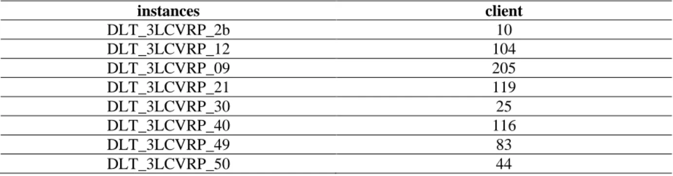
For the classical instances, allowing items rotation slightly improves the results. For this new set of instances, eight instances cannot be solved if rotations are forbidden since the items of some clients cannot be packed with the heuristic we introduced (see Table 13). For one instance, GRASPELS found a solution with 16 vehicles while only 15 vehicles are available.
21
instances client DLT_3LCVRP_2b 10 DLT_3LCVRP_12 104 DLT_3LCVRP_09 205 DLT_3LCVRP_21 119 DLT_3LCVRP_30 25 DLT_3LCVRP_40 116 DLT_3LCVRP_49 83 DLT_3LCVRP_50 44Table 13: Client packing failure with the heuristic if rotations are not allowed
4 Concluding remarks
This article considers an extension of the well-known CVRP in which three dimensional packing constraints must be addressed in each trip servicing clients. This problem deals with two combinatorial optimization problems: vehicle routing and three-dimensional packing. The method we propose compete with the best published methods but the method is currently dedicated to the 3L-CVRP with no extra constraints. It is based on an original resolution of the 3PP based on a dedicated heuristic for the vehicle loading resolution. We are currently investigating the 3L-CVRP with additional constraints, trying to extend the original 3D-packing scheme we introduce.
References
[1] Baldacci R., Battarra M. and Vigo D. Routing a Heterogeneous Fleet of Vehicles. In: The Vehicle Routing Problem: Latest Advances and New Challenges, Golden B. and Wasil E. (Eds). 2008, 3-27. [2] Toth P. and Vigo D. An overview of vehicle routing problems. in: The Vehicle Routing Problem, Toth P
and Vigo D. (Eds). SIAM Monographs on Discrete Mathematics and Applications, Philadelphia, 2002, 1-26.
[3] Prins C. Two memetic algorithms for heterogeneous fleet vehicle routing problems. Engineering Applications of Artificial Intelligence, 2009, 22: 916-928.
[4] Cordeau J.F., Gendreau M., Hertz A., Laporte G. and Sormany J.S. New heuristics for the vehicle routing problem. In: Logistic systems: design and optimization, A. Langevin and D. Riopel (eds.), Wiley, New York, 2005, 279-298.
[5] Gendreau M., Iori M., Laporte G. and Martello S. A Tabu Search Heuristic for the Vehicle Routing Problem with Two-Dimensional Loading Constraints, Networks, 2008, 51(1): 4-18.
[6] Zachariadis E.E, Tarantilis C.D. and Kiranoudis C. A guided Tabu Search for the Vehicle Routing Problem with two dimensional loading constraints, European Journal of Operational Research, 2009, 3(16): 729-743.
[7] Fuellerer G., Doerner K.F., Hartl R.F. and Iori M. Ant colony optimization for the two-dimensional loading vehicle routing problem, Computers and Operations Research, 2009, 36(3): 655-673.
[8] Iori M., Salazar González J.J. and Vigo D. An exact approach for capacitated vehicle routing problems with two-dimensional loading constraints, Transportation Science, 2007, 41(2), 253–264.
[9] Duhamel C., Lacomme P., Quilliot A. and Toussaint H. A multi-start evolutionary local search for the two-dimensional loading capacitated vehicle routing problem, Computers & Operations Research, 2011, 38(3): 617-640.
[10] Gendreau M., Iori M., Laporte G. and Martello S. A Tabu Search Algorithm for a Routing and Container Loading Problem. Transportation Science, 2006, 40 (3): 342-350.
[11] Fuellerer G., Doerner K.F., Hartl R.F. and Iori M. Metaheuristics for vehicle routing problems with three-dimensional loading constraints, European Journal of Operational Research, 2010, 201(3): 751-759.
22
[12] Hifi M., Kacem I.,Nègre S. and Wu L. A Linear Programming Approach for the Three-DimensionalBin-Packing Problem
.
Electronic Notes in Discrete Mathematics, 2010, 36: 993-1000.[13] Wu Y., Li W., Goh M. and de Souza R. Three-dimensional bin packing problem with variable bin height. European Journal of Operational Research, 2010, 202(2): 347-355.
[14] Bortfeldt A. and Mack D. A heuristic for the three-dimensional strip packing problem. European Journal of Operational Research, 2007, 183(3): 1267-1279.
[15] Allen S.D., Burke E.K. and Kendall G. A hybrid placement strategy for the three-dimensional strip packing problem, European Journal of Operational Research, 2011, 209(3): 219-227.
[16] De Almeida A. and Figueiredo M.B. A particular approach for the Three-dimensional Packing Problem with additional constraints, Computers & Operations Research, 2010, 37(11): 1968-1976.
[17] Prins C. A GRASP×Evolutionary Local Search Hybrid for the Vehicle Routing Problem, in: Pereira F.B. and Tavares J. (Eds). Bio-inspired Algorithms for the Vehicle Routing Problem, Studies in Computational Intelligence, publisher Springer, Berlin, 2009, 161: 35–53.
[18] Feo T.A. and Resende M.G.C. Greedy randomized adaptive search procedures, Journal of Global Optimization, 1995, 6: 109–33.
[19] Prins C. A simple and effective evolutionary algorithm for the vehicle routing problem, Computers and Operations Research
,
2004, 31: 1985–2002.[20] Lourenço H., Martin O. and Stützle T. Iterated Local Search. In: Glover F. and Kochenberger G. (Eds). Handbook of Metaheuristics. Springer New York, 2003, 57: 320-353.
[21] Duhamel C., Lacomme P. and Prodhon C. Efficient frameworks for greedy split and new depth first search split procedures for routing problems, Computers & Operations Research, 2011; 38(4):723-739. [22] Gilmore P.C. and Gomory R.E. Multistage cutting stock problems of two and more dimensions,
Operations Research, 1965: 13: 94–120.
[23] Guibas
L.J.
and R. Sedgewick. A Dichromatic Framework for Balanced Trees, 19th Annual Symposium on Foundations of Computer Science, Ann Arbor, Michigan, 16-18 October, 1978: 8-21.[24] Bayer R. and E.M. McCreight. Organization and Maintenance of Large Ordered Indices. Acta Informatica 1972; 1: 173-189.
[25] Lacomme P., Prins C. and Ramdane-Chérif W. Competitive Memetic Algorithms for Arc Routing Problems, Annals of Operations Research, 2004, 131: 159-185.
[26] Beasley J.E. Route-first cluster-second methods for vehicle routing, Omega, 1983, 11: 403–408.
[27] Bajart V. and Charles C. Systèmes d’Information Géographique. 3rd year project report, ISIMA. http://www.isima.fr/~lacomme/students.html, 2009.
23
Appendix 1instance (Gendreau et al., 2006)
(
Fuellerer et al., 2010) GRASP ELS01 297.65 3.40 297.65 1.00 297.65 3.53 297.65 0.0 02 334.96 0.60 334.96 0.10 335.67 0.06 334.96 0.0 03 362.27 448.10 362.27 16.20 362.27 13.99 362.27 0.2 04 430.89 11.10 430.89 0.50 430.88 0.40 430.88 0.0 05 395.64 0.50 406.50 9.60 379.43 8.16 379.43 0.1 06 495.85 14.70 495.85 1.20 495.85 0.30 495.85 0.0 07 742.23 1.80 732.52 18.10 725.43 237.39 725.43 4.9 08 735.14 104.90 735.14 13.30 735.14 36.63 735.14 1.1 09 630.13 977.80 630.13 3.70 630.13 2.18 630.13 0.1 10 717.90 410.70 711.45 92.60 687.57 589.11 687.57 32.1 11 718.24 208.10 718.25 81.90 718.24 1453.35 718.24 1.8 12 614.60 1 302.70 612.63 7.50 610.05 19.66 610.00 2.0 13 2 316.56 2 317.30 2391.77 174.50 2306.04 1242.44 2306.04 86.9 14 1 276.60 2 121.30 1222.17 425.90 1186.96 2423.64 1184.44 3600.2 15 1 196.55 2 916.14 1182.86 645.00 1161.20 2144.72 1161.11 689.3 16 698.61 863.00 698.61 2.80 698.61 2.87 698.61 0.0 17 906.42 753.20 862.18 3.10 861.80 8.58 861.79 1.2 18 1 124.33 2198.90 1112.18 1484.60 1084.26 1893.69 1078.41 2030.8 19 680.29 1 390.30 671.60 414.40 670.44 3322.67 658.34 3429.6 20 529.00 7 007.50 515.39 1436.70 510.95 2892.97 503.30 1469.7 21 1 004.40 6 262.50 951.87 2105.70 943.05 4173.74 921.25 4697.4 22 1 068.96 2 078.70 1030.12 1218.40 1029.87 3561.80 1009.45 3348.3 23 1 012.51 4 314.10 971.05 1231.70 987.06 3120.66 976.46 1889.1 24 1 063.61 1 052.50 1057.39 184.70 1056.33 2610.20 1047.75 682.8 25 1 371.32 500.90 1207.97 3986.10 1232.73 4489.01 1219.77 4658.4 26 1 557.12 1 075.00 1453.39 2843.60 1415.15 3484.63 1393.76 3066.6 27 1 378.52 3 983.20 1333.16 2208.30 1317.38 3372.87 1304.82 2422.3 Avg. Cost 876.31 856.67 847.04 841.96 Avg. Time 1567.4 689.3 1522.56 1189.44 Avg. Norm. Time 1504.1 689.3 1004.89 785.03
24
instance GRASP ELS GRASP ELS
Rotations allowed Rotations forbidden
01 297.65 3.53 297.65 0.0 297.65 1.01 297.65 0.0 02 335.67 0.06 334.96 0.0 335.67 0.06 334.96 0.0 03 362.27 13.99 362.27 0.2 362.27 5.31 362.27 0.2 04 430.88 0.40 430.88 0.0 430.88 0.19 430.88 0.0 05 379.43 8.16 379.43 0.1 379.43 1.56 379.43 0.0 06 495.85 0.30 495.85 0.0 495.85 0.34 495.85 0.0 07 725.43 237.39 725.43 4.9 732.51 104.85 732.51 0.1 08 735.14 36.63 735.14 1.1 730.66 115.78 730.66 0.1 09 630.13 2.18 630.13 0.1 633.72 2.52 633.72 0.1 10 687.57 589.11 687.57 32.1 704.97 1009.19 704.64 34.2 11 718.24 1453.35 718.24 1.8 718.24 225.10 718.24 13.6 12 610.05 19.66 610.00 2.0 610.00 11.62 610.00 2.7 13 2306.04 1242.44 2306.04 86.9 2299.05 111.17 2299.05 3.9 14 1186.96 2423.64 1184.44 3600.2 1194.57 2966.97 1192.29 612.0 15 1161.20 2144.72 1161.11 689.3 1163.34 1975.90 1163.23 1050.3 16 698.61 2.87 698.61 0.0 700.80 1.20 700.80 0.1 17 861.80 8.58 861.79 1.2 861.79 7.69 861.79 2.2 18 1084.26 1893.69 1078.41 2030.8 1091.61 2502.66 1091.28 4137.8 19 670.44 3322.67 658.34 3429.6 665.45 2489.16 662.96 1810.9 20 510.95 2892.97 503.30 1469.7 515.95 2340.49 513.28 3166.3 21 943.05 4173.74 921.25 4697.4 947.30 2503.90 940.72 2945.8 22 1029.87 3561.80 1009.45 3348.3 1039.64 2249.58 1021.02 3552.4 23 987.06 3120.66 976.46 1889.1 980.63 2194.71 972.12 3146.3 24 1056.33 2610.20 1047.75 682.8 1053.60 3964.98 1048.55 3697.1 25 1232.73 4489.01 1219.77 4658.4 1224.56 2898.75 1209.81 2564.6 26 1415.15 3484.63 1393.76 3066.6 1427.58 3053.36 1421.35 4711.4 27 1317.38 3372.87 1304.82 2422.3 1322.02 2449.77 1298.84 3617.4 Avg. Cost 847.04 841.96 848.88 845.48 Avg. Time 1522.56 1189.44 1229.18 1298.87
25
Appendix 2 GRASP ELS DLT_3LCVRP_01 Ain 1461.63 5361.81 1388.27 5418.4 DLT_3LCVRP_08 Ardennes 1065.51 2764.31 1041.54 2461.0 DLT_3LCVRP_10 Aube 1232.45 3685.94 1200.33 2580.6 DLT_3LCVRP_11 Aude 1565.7 4491.45 1517.85 4854.3 DLT_3LCVRP_36 Indre 2085.69 4594.17 2042.01 5324.0 DLT_3LCVRP_39 Jura 1828.25 4174.64 1758.5 5076.3 DLT_3LCVRP_43 Haute Loire 1361.26 4117.87 1317.93 5301.0 DLT_3LCVRP_52 Haute Marne 1176.91 3635.08 1146.78 2618.0 DLT_3LCVRP_55 Meuse 1103.22 2458.72 1078.8 1526.2 DLT_3LCVRP_70 Haute Saone 1328.27 3777.12 1289.68 5052.7 DLT_3LCVRP_75 Paris 71.6 78.82 71.6 1.3 DLT_3LCVRP_82 Tarn et Garonne 1027.84 3704.84 1006.8 5135.5 DLT_3LCVRP_92 Haut de Seine 256.88 2454.46 254.56 133.4 DLT_3LCVRP_93 Seine saint denis 219.44 3020.38 216.35 4722.1 DLT_3LCVRP_94 Val de Marne 254.01 3614.27 242.04 2581.4Average 1069.24 3462.26 1038.20 3519.08