Determination of optimal safety stock levels for components in an instant film assembly system

Determination of Optimal Safety Stock Levels for Components in an Instant Film Assembly System

by John J. Wilson

B.S. Physics

United States Naval Academy, 1989 Submitted to the Sloan School of Management and the Department of Mechanical Engineering in Partial Fulfillment of the Requirements for the Degrees of

Master of Science in Management and

Master of Science in Mechanical Engineering at the

Massachusetts Institute of Technology June 1996

@ 1996 Massachusetts Institute of Technology All rights reserved.

Signature of Author ... _{... ... .. Depat of o • . hanical . y'/ " :4:. Engineering. .}

May 10. 1996 Certified by ... ... v. ... . ... .... 1 Vien Nguyen Associate Professor of Management Science Certified by ...

I John Tsitsikilis

/ Professor of/Electrical Engineering Certified by ...

Stanley B. Gershwin Senior Research Sci t Department of Mechanical Engineering

Accepted by ...

Ain Sonin

OF TECHNOLOGY Chairman, Department Committee Department of Mechanical Engineering

JUN

2 61996

_Eng.

Determination of Optimal Safety Stock Levels for Components in an Instant Film Assembly System

by

John J. Wilson

Submitted to the Sloan School of Management and the Department of Mechanical Engineering on May 10, 1996

in Partial Fulfillment of the Requirements for the Degrees of Master of Science in Management and

Master of Science in Mechanical Engineering Abstract

Manufacturing systems are subject to uncertainties caused by less than perfectly reliable production processes and unpredictable demand patterns. Safety stocks of finished goods inventory can serve to buffer against these uncertainties, and therefore reduce the

likelihood of incurring a penalty cost created by a material stockout. However, holding large inventories entails certain costs as well. Thus, an optimal level of inventory safety stock must trade off the costs of holding inventory against the benefits of improved service level, in order to minimize the total expected value of holding cost and penalty cost. This thesis analyzes the uncertainties faced by a manufacturer of components for instant film, and develops a revised inventory policy for the manufacturer based upon that analysis. It is shown that the optimal level of inventory safety stock can be significantly reduced by holding the photographic component inventory in a format which can flexibly

be used to satisfy demand for a set of product lines in a given product family. In addition,

the thesis includes the construction of a simulation model which accurately reflects the uncertainties faced by the component manufacturer. Repeated simulations have been conducted to determine the safety stock level which results in the lowest expected value for the sum of inventory holding and penalty costs.

Thesis Supervisors: Vien Nguyen, John Tsitsikilis

Acknowledgments

First, I must thank my wife Kim for all of her support during my two years at MIT. During this time, she courageously worked hard to pay the bills, gave birth to our

daughter Katie, and then worked even harder to provide a good home for our new baby. She did all of these things while also being patient with me as I struggled to reach a healthy balance between schoolwork and family life. I love you Kim.

Next, I want to acknowledge my Mom and Dad for all of their encouragement and support over the years. As a new parent, I am now able to better recognize the enormous portion of their lives which they have devoted to helping my brother and me. Thanks Mom and Dad.

In addition, I would like to thank my brother Rob for being such a great friend to me. Also, I should mention that upon graduation from MIT I will have (at least) equaled my esteemed brother in terms of academic accomplishments.

Finally, I must thank all of the people at MIT and at Polaroid that helped me generate this thesis. Vien Nguyen, John Tsitsikilis, and Stan Gershwin were all very helpful advisors. Tom Denoto, Gary Crago, and Amy Blake of Polaroid Corporation ensured that thy time at Polaroid was not only useful but also fun.

The author wishes to acknowledge the Leaders for Manufacturing Program for its support of this work.

Contents

1 Introduction

1.1 Problem Description ... ... ... ... 9

1.2 Description of Manufacturing Process Flow for Instant Film ... 10

1.3 Production Planning Methods for Instant Film ... 12

1.4 Problem Solving Approach ... 13

1.5 The Nature of Production Process Reliability in Building 1 ... 15

1.6 Outline of Thesis Contents ... 16

2 Selected Literature Review

2.2 M RP System Basics ... ... ... ... 20

2.3 Safety Stocks in MRP Systems ... ... 21

2.4 The "Just in Time" Inventory Philosophy ... 25

2.5 Analytical Determination of an Optimal Inventory Policy ... 26

2.5.1 The Utility of an Analytical Solution ... 26

2.5.2 Deriving the Analytical Solution- The Hedging Point Policy ... 27

3 Lower Inventories and Higher Service Levels:

The Benefits of Risk Pooling

3.1.1 Special Case of Two Independent Random Variables ... 33

3.1.2 Special Case of Two Perfectly Correlated Random Variables .... 34

3.1.3 The Variance of the Sum of Many Random Variables ... 35

3.1.4 Exploiting the Concept of Risk Pooling ... 36

3.2 The Benefits of Risk Pooling at Building I ... .... ... 40

4 Simulation Model of Photographic Media Production and Demand

4.1 Simulation Model Assumptions ... 49

4.1.1 Assumptions for System Operating Policy ... 49

4.1.2 Assumptions for the Random Nature of Production and Demand .. 53

4.2 Using the Simulation Model ... ... 57

4.2.1 Inputs to the Simulation Model ... ... 58

4.2.2 Outputs of the Simulation Model ... ... 60

4.3 Results of Simulation Analyses ... 63

4.3.1 Baseline Scenario ... .... ... 63

4.3.2 Determination of the Baseline "Optimal" Inventory Policy ... 66

4.3.3 The Impact of Holding and Penalty Costs on Optimal Inventories .. 71

4.3.4 The Impact of Safety Stock Levels on Service Levels ... 72

4.3.5 The Impact of Capacity / Demand Parameters on Service Levels .. 73

4.3.6 Year to Year Variability of System Performance ... 76

4.4 Capacity Allocation Issues in Multi-Product Manufacturing Systems ... 79

5

Application of the Hedging Point Model to Polaroid's

Component Manufacturing

5.2 The Optimal Hedge Point for the Baseline Scenario ... 84

5.3 The Impact of Capacity / Demand Parameters on the Hedge Point ... 86

5.4 The Impact of Process Reliability Parameters on the Hedge Point ... 88

6

Conclusions

6.2 A Holistic View of Supply Chain Inventories ... 93

6.3 The Impact of Financial Metrics on Inventory Policies ... 93

Appendix

...

...

94

Chapter 1

Introduction

1.1 Problem Description

Manufacturing systems are subject to uncertainties caused by less than perfectly reliable production processes and unpredictable demand patterns. Safety stocks of finished goods inventory can serve to buffer against these uncertainties, and therefore reduce the likelihood of incurring a penalty cost created by a material stockout. However, holding large inventories entails costs as well. Thus, an optimal level of inventory safety stock must tradeoff the costs of holding inventory against the benefits of improved service level, in order to minimize the total expected value of holding cost and penalty cost. This thesis focuses specifically on determining an optimal inventory policy for one of Polaroid

Corporation's instant film component manufacturing facilities. However, the insights gained as a result of this work are relevant to manufacturing systems in general.

To fully understand the issues involved in determining a safety stock policy for Polaroid's component manufacturing facility, it is necessary to describe the manufacturing process for instant film. It is also important to examine the instant film production planning methods. Sections 1.2 and 1.3 provide the necessary background in these areas. Then, Section 1.4 outlines the approach we have developed for the determination of an inventory policy which minimizes Building l's expected holding and penalty costs. Section 1.4 also provides an overall outline of the thesis contents.

1.2 Description of the Manufacturing Process Flow for Instant Film

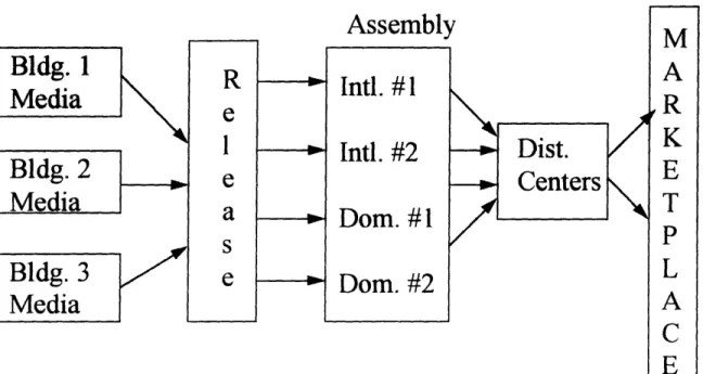
The manufacture of instant film at Polaroid is a highly complex process carried out at numerous different locations. However, in its simplest form, the entire process for film manufacture consists of three basic steps:

1) The three main components of instant film (the positive sheet, the negative, and the

chemical developer) are manufactured according to their own specifications.

2) Each set of components intended to be joined at assembly must be tested together to ensure satisfactory total system performance. This procedure is termed the "release" step.

3) A "released" set of components is then assembled to produce the instant film.

Assembly is accomplished both domestically and internationally, at a total of four different locations.

A schematic of the film manufacturing process is shown below in Figure 1.1. For the

purposes of confidentiality, the identity of the specific components manufactured at each location is not revealed.

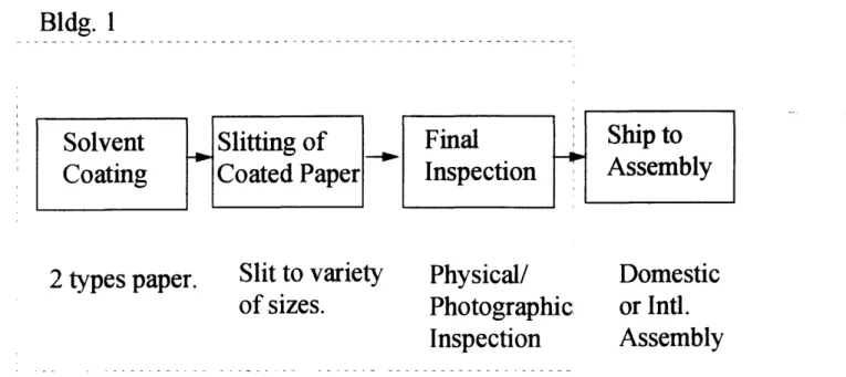
This research has focused upon the inventory policy for the photographic media manufactured in Building 1. Figure 1.1 illustrates Building l's role in the overall manufacture of instant film. Figure 1.2 illustrates the photographic media production process performed within Building 1. Three basic steps are required to manufacture the photographic media.

1) Rolls of paper are sequentially coated with various chemical layers to impart the

necessary photographic characteristics to the material. There are two types of paper, which are used for two different families of products.

2) The coated rolls of paper (referred to as "full web" rolls) are slit to various different widths, depending on the size of the picture to be made. Samples are removed for inspection during the slitting step.

3) The samples are inspected to check for both physical defects and photographic

acceptability.

Bldg. 1

2 types paper.

Slit to variety

of sizes.

Physical/

Photographic:

Inspection

Domestic

or Intl.

Assembly

The two types of paper used in the coating process are similar except in thickness. Thick paper is used for large formats of instant film, whereas thinner paper is used for the smaller picture sizes. Lastly, we note that although only two types of paper are coated, there are six different sizes for instant film (e.g. 8"X10", 5"X7", 4"X6").

1.3 Production Planning Methods for Instant Film

Polaroid Corporation uses an MRP (material requirements planning) system to plan the production of instant film. Each assembly plant establishes a production schedule based on a rolling forecast of demand. Then, assembly plant material managers calculate the quantity of components necessary to support the scheduled film production. Since Building 1 supplies multiple assembly plants, it must schedule production of photographic media based upon the aggregated requirements of all the assembly plants. Building l's MRP system translates future requirements for photographic media into a production

schedule for the coating process, assuming that standard process yields and nominal production lead times will be achieved.

It is important to note that assembly plant orders for components are generally required to be placed in advance of their required due date by a minimum of one production lead time. Therefore, Building I is able to schedule and complete a production campaign to precisely match the quantity demanded by the assembly plants. Polaroid refers to this requirement as a "time fence" policy, since no order changes are allowed inside of a fixed time interval. This policy is intended, in part, to prevent one assembly plant from making unreasonable last minute requests for extra components that may be received only at the expense of another assembly plant. In addition, the policy prevents Building 1 from having to incur excessive overtime expenses that could result from frequent last minute order changes.

Targeted levels of inventory safety stocks exist for each different product line. If the on hand inventory levels are equal to the desired safety stocks, Building I will produce exactly that quantity of material necessary to supply the assembly plants. However, if

inventory is less than the desired level, extra material will be produced to build each product's inventory to the targeted value. Currently, all safety stock is held in product specific formats; that is, the safety stock of material is slit to the shape of a specific product line and inspected to assure satisfactory quality.

1.4 Problem Solving Approach

In deciding upon an inventory safety stock policy, we must consider three basic issues. First, how much does it cost to hold a given safety stock of material? Next, what are the penalty costs associated with a material shortfall? And lastly, how often would we expect to suffer a stockout (and therefore incur some penalty cost) for a given

inventory policy? Unfortunately, it is often difficult to precisely determine any of the parameters above. Nevertheless, for the case of Building 1, we can easily establish a range of reasonable values for inventory holding and penalty costs. The larger challenge is to anticipate the service level performance of a given inventory policy.

The ability of Building 1 to meet the demands of its customers will depend not only on the quantity of inventory safety stock held, but also on the reliability of its

production process and the nature of the demand it faces. Specifically, we recognize that inventory safety stock is necessary for Building 1 to protect against material shortages in the event of:

a) a last minute upward revision of a demand requirement from an assembly plant

b) a periodic demand for photographic media which exceeds Building l's capacity

c) a production problem within Building 1.

If we consider that Polaroid's "time fence" policy is strictly enforced, then Building 1

does not need to hold inventory to buffer against last minute order quantity revisions. Furthermore, if we discover that the demand each week is almost always less than capacity, then we realize that inventory safety stock is necessary only to buffer against potential production problems. Under these circumstances, we may argue that if the

production process at Building 1 were perfectly reliable, then no inventory safety stock would be necessary.

Of course, there is not any real world production process that is perfectly reliable,

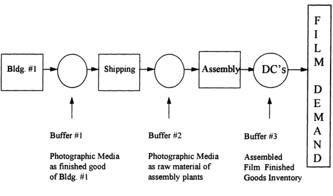
and the production process for photographic media at Building I is no exception. But, the above analysis allows us to better understand the reasons why Building 1 must hold a safety stock of material. Consider the following simplified diagram of the instant film supply chain. The diagram does not show all the assembly plants, nor all the component manufacturers.

Buffer #1 of Bldg. #1

Buffer #2 Buffer #3

assembly plants Goods Inventory

Figure 1.3 Simplified schematic of the instant film supply chain.

Based upon the above discussion, we now recognize that the inventory in Buffer #1 above is useful primarily to protect against potential production problems in Building 1.

Moreover, since the assembly plants are generally not allowed to make last minute revisions to their component requirements, Buffer #2 above is useful to allow for short

term increases in the production schedule of the assembly plants. (Such a change to the assembly plant schedule may be necessary if the error in the forecasted film sales for a given period were large.)

1.5 The Nature of Production Process Reliability in Building 1

Less than perfectly reliable production processes require manufacturing systems to hold inventory safety stock. The quantity of safety stock necessary to buffer against production problems depends upon the frequency and duration of the process failures. We consider two distinct types of production process interruptions:

1) One or more machines in a process may suffer a failure precluding them from operating. The process is interrupted until the machines are repaired. No material is produced during this time.

2) All production process machines are operating, but the quality of material being produced is unacceptable. Thus, little or no usable material is being produced during some time interval of operation.

In the case of Polaroid's manufacturing operations in Building 1, the latter case is of greater concern. When a piece of machinery has failed and is not capable of being

operated, repair personnel are able to quickly repair the faulty equipment. However, when all machines are operating but producing poor quality material, it is possible that the process will be allowed to continue in such a state for an extended period of time. Thus, this type of process "quality failure" is generally not "repaired" as quickly as the machine operating failures described above.

We demonstrate in Section 5.4 that infrequent, long duration process failures create the need for more inventory safety stock than frequent, short duration failures. Thus, our analysis of the production process uncertainty in Building 1 will focus on the

process quality failure described above. Polaroid Corporation manufacturing managers describe such an event as a process "excursion". In subsequent portions of the thesis, an excursion is taken to be the occurrence of a long duration failure during which the process is unable to produce material of acceptable quality.

1.6 Outline of Thesis Contents

The substantial portion of this research focuses upon determining an optimal value for the inventory to be held in Buffer #1 of Figure 1.3 above. We do not examine the distribution of errors in the forecasted film sales, and we therefore do not attempt to calculate an appropriate level of component inventories for the assembly plants to hold.

Similarly, we do not address the issue of determining an appropriate level of finished goods inventory to hold in the distribution centers.

In order to estimate an optimal inventory safety stock of media for Building 1 (Buffer #1 above), we collected historical data to quantify the reliability characteristics of the photographic media production process. Similarly, we examined the historical

distribution of demand faced by Building 1. Armed with this knowledge, and an estimate of reasonable values for holding and penalty costs, a computer simulation was constructed to model the performance of various different inventory safety stock policies. Repeated runs of the simulation allow the user to search for an optimal policy. Chapter 4 describes the simulation model in detail. Then, Chapter 5 compares our simulation model results with those obtained from an analytical solution of a simplified but similar manufacturing system.

In addition to the simulation model, significant work was performed to demonstrate the benefits to Building 1 of holding its inventory in a "full web" format, rather than holding inventory in a product specific, slit format. A full web inventory policy allows Building 1 to flexibly and efficiently utilize the safety stock of material, in exactly the mix of product formats demanded. Furthermore, such a policy pools the variability of demand for all the product lines of a given product family. Chapter 3

Lastly, Chapter 2 provides brief review of some of the literature on inventory safety stocks. There has been an enormous amount of material written on this subject, and

I have not intended to provide a comprehensive review. Rather, the documents discussed

have been chosen because they seemed particularly relevant to the specific inventory issues faced by Polaroid's component manufacturers.

Chapter 2

Selected Literature Review

It is not the intention of this chapter to provide a comprehensive review of the literature on inventory safety stocks in manufacturing systems. For the interested reader, Graves (1988) provides an excellent summary of this body of research. Our purpose here is to highlight a portion of the literature which seems particularly relevant to the situation faced by Polaroid's component manufacturing facilities.

2.1 The Definition of Inventory "Safety Stock"

Factories must necessarily hold inventories of raw materials, work-in-process, and finished goods. Graves (1988) describes the following reasons why these inventories are

necessary:

1) Pipeline stock is the inventory in a manufacturing system that exists because of the time required to process material in a given procedure, and because of the time required to

transport the material from one stage of the system to another. In order to reduce the pipeline stock in a system with a fixed production rate, it is necessary to reduce the time required for processing or transporting material. Specifically, Little's Law states that

L=XW

where L = the average pipeline stock in any given system

X = the average production rate of the system

W = the average time material spends in the system

2) Cycle stock is the inventory in a manufacturing system that exists because production and ordering processes are batch operations. In order to reduce the cycle stock, the batch size of operations must be reduced.

3) Anticipation stock is the inventory in a manufacturing system intended to smooth the

required production rate in the event of a seasonal demand peak exceeding system capacity. To reduce the anticipation stock, the system production must be more closely matched with the cumulative demand placed upon it.

Graves defines "safety stock" to be the system inventory held in excess of the pipeline, cycle, and anticipation stocks. More specifically, safety stocks are the "excess inventories held beyond the minimum inventory level that would be possible in a

deterministic and uncapacitated world." Safety stocks are necessary because

manufacturing systems operate in an environment of uncertainty. Production processes are generally not perfectly reliable; similarly, demand processes can not be forecasted with perfect accuracy. Manufacturing systems with finite production capacities may not easily recover from the disturbances caused by unforeseen production or demand events. Safety stocks are used to mitigate the negative impacts of such disturbances.

Having now established a working definition of inventory safety stock, we will specifically discuss the issue of safety stocks in a manufacturing system which uses Materials Requirements Planning (MRP).

2.2

MRP

System Basics

The operation of an MRP system can be simply described as follows (Orlicky, 1975). The components required to manufacture a given product are delineated in a Bill of Materials. Using the information within the Bill of Materials, forecasted demand for end product items can be directly translated into quantity requirements for individual

components by means of an explosion calculus. Similarly, the nominal production lead times for each manufacturing process are entered into the MRP system. Using these nominal lead times, the explosion calculus determines the time period in which a component must begin to be made, in order to be ready for final assembly at the required time. Thus, by starting with a forecasted demand for the final product, we can generate a Master Production Schedule which details the quantities of parts which must enter

production at each time interval to meet the anticipated end-item demand.

The most straightforward execution of the above process utilizes a lot-for lot replenishment system. In this case, every period's scheduled production of parts is exactly equal to the time-phased requirements calculated above. Alternatively, we could choose to manufacture more than one period's forecasted requirements for some components, and thereby eliminate the need to make these components each and every period. This alternative policy of producing larger lots of material less frequently will in some cases be more economical than the simple lot-for lot method. The choice of lot sizing policy will depend upon the cost of holding the components made in excess of the immediate requirements, and upon the cost of performing a manufacturing setup to begin production of these parts. In general, high-cost setups will tend to make larger lots more desirable. For the special case of a forecasted demand requirement which is fixed over a

certain planning horizon, it is easy to calculate the optimal lot sizing rule, which will minimize the sum of setup costs and inventory holding costs. Wagner and Whitin (1958)

have shown that for a deterministic time varying demand, the optimal lot sizing policy will produce a quantity of parts at every period that is exactly equal to the sum of a set of future demands. Therefore, the determination of an optimal lot sizing policy over this

time horizon may be cast as a shortest path dynamic programming problem that has only a very small number of feasible solutions.

The methodologies described above seem to constitute a very logical system for scheduling production. However, it is important to recognize that some of the

assumptions of the MRP system may not accurately reflect a real world manufacturing system. Nahmias (1993) highlights the following issues:

1) The explosion calculus assumes that the forecasted end-item demand will be precisely

realized. In reality, there will likely be some forecast error. Errors in forecasted end-item demand generate errors in the individual component requirements calculated by the MRP system.

2) MRP systems assume that the production lead time for any given part is fixed, known in advance, and independent of the lot size to be manufactured. We may more realistically expect that larger lot sizes will require more time to produce. Moreover, there may be some uncertainty associated with the time required to complete a production run of any given size.

3) The explosion calculus assumes that the quantity of acceptable parts produced in any

given batch is known in advance. If all production yields are stable, this is a fair assumption. However, uncertain yield rates may exist for some processes.

The issues described above should provide some insight into the need for safety stocks in an MRP system. Section 2.3 discusses this issue in more detail.

2.3 Safety Stocks in MRP Systems

Recall from Section 2. 1 that safety stocks are required to buffer against the impact of production and demand uncertainties. For the specific case of an individual component manufactured within an MRP system, Whybark and Williams (1976) classified these uncertainties as follows:

1) Demand quantity uncertainty - In any given time period, the quantity required of a given part may be different from the planned requirement. Demand quantity uncertainty may result from forecast errors which require a revision of the Master Production

Schedule.

2) Demand timing uncertainty - The expected demand requirements for a given part may shift in time. Demand timing uncertainty may result from changes in the promised delivery date to one or more customers.

3) Supply quantity uncertainty -In any given time interval, the quantity of parts available for use may be different from the planned quantity. Supply quantity uncertainty may result from unstable yield rates for various in-house manufacturing processes, or from vendors who fail to deliver a promised quantity of raw materials.

4) Supply timing uncertainty -An expected set of parts may not be available for use exactly when expected. Supply timing uncertainty may result from the variability of in-house production process lead times, or from vendors who fail to deliver raw materials on time.

It is interesting to note that many early proponents of MRP shared the view of Orlicky (1975) that inventory safety stocks were not necessary in a well run MRP system, except at the end-item level. Graves (1988) speculates that this belief is likely a direct result of most MRP systems' inability to consider the uncertainties above. However, he points out that this view is no longer well accepted, as evidenced by the large number of papers written on the topic of safety stocks in MRP systems. Wemmerlov (1979)

surveyed thirteen firms using MRP systems, and found that the majority held inventory in other than end-item form. Such a policy can potentially reduce inventory holding costs because the material is less valuable than the finished products, and because component commonality may reduce the quantity of safety stock required. (Chapter 3 discusses in

detail the safety stock reductions that can be achieved by holding an inventory of components which are common to numerous product lines.)

The literature on safety stocks in MRP systems generally includes three basic methods for buffering against the above uncertainties. First, a fixed level of desired safety stock can be established for each part. In this case, the MRP system will generate

production requirements for the parts whenever the planned inventory level (calculated by matching the current work orders against the forecasted requirements) drops below the targeted safety stock. The planned order quantity will be set so as to re-establish the targeted buffer level for the part. Secondly, a fixed interval of safety lead time may be established for any given part. In this case, the MRP system simply calculates production requirements such that parts will arrive at some fixed interval prior to their forecasted need. Lastly, Miller (1979) proposed that the end-item demand may be purposefully inflated (or "hedged") to account for uncertainties in the forecast. In this case, the explosion calculus will cause the deliberately overplanned end-item demand to be transmitted into extra requirements for lower level parts.

New (1975) provides an excellent qualitative analysis of the issues to consider when determining safety stocks or safety lead times in MRP systems. In addition, he discusses the relative advantages of safety stock versus safety time. He makes a strong argument for the advantage of safety lead time in the case of a part which is only

infrequently produced. This result makes intuitive sense, since the use of a safety lead time will cause the system to hold a safety stock of material only when a real requirement for the part exists in the near future. Whybark and Williams (1976) conducted numerous simulation analyses to compare the effectiveness of safety stock policies versus safety lead time policies. They found that safety lead times were generally better at buffering against timing uncertainties, while safety stocks were more effective in buffering against quantity uncertainties.

Meal (1979) expanded upon the qualitative work of New( 1975) and others to propose a quantitative method for establishing safety stocks and safety lead times in an MRP system. Meal considers the four sources of uncertainty outlined by Whybark and Williams (1976) and demonstrates a methodology for quantifying the magnitude of these

uncertainties. Specifically, Meal proposes that the uncertainties facing a manufacturing system can be estimated from the distribution of the errors in past forecasts. In order to examine these error distributions, manufacturers would be required to keep records not only of the actual requirements (and actual supply) for each part over time, but also of the forecasted requirement (and forecasted supply) for these parts. Lastly, Meal argues that the quantity and timing uncertainties may be treated independently. He recommends combining the supply and demand quantity uncertainties to determine a safety stock for a given part; similarly, he combines the supply and demand timing uncertainties to determine safety time.

Miller (1979) suggests that the end-item demand be overstated as follows. Consider a stationary, normal, and independent end-item demand with mean g and standard deviation a. In this scenario, the forecasted demand for this item will be ýt for all time periods; the distribution of forecast error will have mean zero, and standard deviation a. The Master Production Schedule is hedged by scheduling the cumulative

end-item production for the next z time periods to be given by t ýt + Z a zr, for all values

of t. The parameter Z is chosen to provide some expected service level based upon the standard normal probability distribution. (For example, Z= 1.645 would presumably provide a 95% service level.) This process will result in safety stocks of material being held at all stages of the production system. Specifically, Miller shows that the expected inventory at each stagej will be given by

E(1j) =Z o( 4LTj- 4Ltj.,)

where LTj is the time required to complete the production of the end-item from stage j.

Guerrero (1986) compared Miller's "pipeline hedging policy" to that of a policy with exclusively end-item safety stock. He found that total inventory required for a given service level was approximately the same in both cases. However, since end-item goods are generally more costly, the pipeline hedging policy may be more attractive for some product cost structures. Lastly, Graves (1988) has demonstrated that Miller's pipeline hedging model will not deliver precisely the end-item service levels implied by the service factor Z above. He does not, however, claim that the underperformance is so great as to necessarily render the policy ineffective.

2.4 The "Just In Time" Inventory Philosophy

The above discussion has focused on methods for determining appropriate levels of inventory safety stocks in a manufacturing system operated under Materials

Requirements Planning. Since safety stocks are necessary to buffer against uncertainties in the manufacturing environment, Section 2.3 specifically focused upon the sources of uncertainty present in an MRP environment. However, we must recognize that all manufacturing systems, regardless of the management system in place, include some elements of uncertainty. The Just-In-Time (JIT) manufacturing philosophy emphasizes the importance eliminating (or minimizing) these uncertainties, so that inventory safety stocks will no longer be necessary. It is important to realize that the elimination of uncertainties in the manufacturing environment is the goal of JIT, and that the elimination of inventory safety stocks is merely a byproduct of achieving that goal.

Proponents of JIT view inventory safety stock as being inherently evil (Hay,

1988). Specifically, they point out that buffers of inventory intended to minimize the

impact of production process problems may actually serve to hide these problems from view, and therefore reduce the likelihood of anyone taking steps to solve them. In order to illustrate this point, JIT proponents use the following analogy: Consider the factory to be a lake, and the problems in the factory to be rocks at the bottom of the lake. In this analogy, inventory safety stock is the water in the lake which hides the rocks from our view. The goal of the manufacturing manager in a JIT environment is to solve the problems in the factory (remove the rocks from the bottom of the lake) so that the

inventory safety stock levels may be reduced (the water in the lake is no longer necessary to cover up the rocks).

It is vitally important that the uncertainties in the manufacturing environment be reduced before the inventory safety stocks are eliminated. It is true that immediate inventory reductions will help to better expose problems in the factory; however, such inventory reductions may also make the entire manufacturing system vulnerable to minor production problems at any given stage. In the words of one former MIT student, "Reducing inventory to find trouble spots in a factory is like walking barefoot to find

broken glass." In summary, the JIT philosophy has correctly emphasized the importance of minimizing the uncertainties in a manufacturing environment. But, as long as

substantial uncertainties do exist, inventory safety stock provides a necessary and desirable buffer against these uncertainties.

2.5 Analytical Determination of an Optimal Inventory Policy

Section 2.3 qualitatively described the sources of uncertainty which are present in an MRP manufacturing environment. Section 2.4 stated that all manufacturing systems are subject to uncertainties, and therefore that some unspecified level of inventory safety stock is generally desirable. Here, we describe an analytical method for precisely determining an optimal inventory safety stock policy for a simple manufacturing system subject to uncertainty under a strict set of assumptions. The policy is optimal because it minimizes the sum of inventory holding and penalty costs. This is in contrast to a great deal of the literature on safety stocks, which does not consider the costs of holding inventory or missing orders, but rather strives to determine the inventory necessary to reach a desired service level.

Bielecki and Kumar (1988) derived the analytical solution presented below. Gershwin (1994) provides a clear review of their work, and the following discussion is based largely upon that review.

2.5.1 The Utility of an Analytical Solution

Unfortunately, the complexity of most real world manufacturing systems precludes us from analytically solving for an optimal inventory policy. The simple system we

describe here is not intended to capture all of the complexities of a real world system.

Rather, the system is carefully constructed to reasonably reflect certain key elements of uncertainty in the manufacturing environment, and yet still be mathematically tractable. Therefore, the utility of this model is not in its ability to determine optimal inventory policies for real world manufacturing systems. Instead, the solution of this simple system is useful because it provides us with insight into the general behavior of the optimal inventory policy as we vary certain parameters.

2.5.2 Deriving the Analytical Solution- The Hedging Point Policy

Consider a manufacturing system with a single machine, capable of producing a single type of part. While the machine is operating, it has a maximum production capacity of . parts per unit time interval., although it can be operated at any

rate u, subject to 0 <= u <= jp. Moreover, the machine is not perfectly reliable. We

assume an exponentially distributed mean time to machine failure given by MTTF = (1/p)

unit time intervals; similarly, we assume the time to repair the machine is exponentially distributed with MTTR = (l1r) unit time intervals. This means that the probability of a machine failure occurring in any small time interval of operation 6t is given by p8t, and the probability of a machine repair occurring in any small time interval of downtime 6t is

given by r St. If we let a(t) = 1 if the machine is operating, and a(t) = 0 if machine is

down, then we may write:

Prob ( ca(t+8t ) = 0 a(t)= 1 ) =pt

Prob ( a(t+t ) = 1 a(t) = 0 ) = r8t

Under these assumptions, the machine is expected to be operating a fraction of the time given by

Prob (a(t) = 1) = Fraction uptime = r / ( r +p )

Therefore, the maximum long term average of the machine's production rate is

Maximum average production rate = rp / ( r + p )

Now consider that the single machine must satisfy a constant demand of d parts per unit time, where d is constrained be less than the maximum average production rate of the machine. Then, define x (t) to be the cumulative difference between the quantity of parts produced and the quantity of parts demanded at time t. Thus, x (t) > 0 means that an inventory of extra parts is on hand, x (t) < 0 means that a backlog exists. (Note that demand is assumed constant for all time, regardless of the quantity of parts on hand.

Thus, we are assuming that the inability to satisfy demand from stock results in backlogs, not any lost orders.) Lastly, we assume that the cost of holding inventory and the cost of incurring a backlog can be precisely specified on a "per unit-per time" basis. At each time interval, an inventory holding cost is incurred if x (t) is greater than zero, and a penalty cost is incurred ifx (t) is less than zero. We define the following variables:

g9 = per unit -per time cost of holding inventory

g. = per unit -per time cost of a backlog

x÷ = x (t) ifx (t)> 0, and x = 0ifx(t) < 0 x7 =-x (t) if x(t)< 0, and x =Oifx(t) 2 0

Based on the definitions of the above, we see that the total cost per unit time incurred by the system may be written as a function of x (t). Specifically, the total cost per unit time is

g (x) = g+ x' + g. x

Therefore, the cost incurred over some time interval (t 1,t2) is given by

t2

Total Cost = J g (x(t) ) dt

tl

The objective of an optimal inventory policy is to minimize the expected value of holding and penalty costs over some very long time interval. Since demand is assumed to be constant, the selection of an inventory policy is equivalent to the selection of a production rate policy for the machine. Thus, the problem of determining an optimal inventory policy in this scenario may be represented by the following dynamic

programming problem. We must choose the machine's production rate u(t) as a function of the system state (x (t), a (t) ), for all times 0<t<T, in order to

T

minimize E [

f

subject to:

dx / dt = i - d

0 <=11 <=

pýca

Prob ( a(t+8t ) = 0 a(t) = 1 ) =pt

Prob ( a(t+8t )= 1 I (t) = 0 ) = r6t

Bielecki and Kumar assume that T is very large. Thus, the minimization above will give us the production rate which provides the lowest long term expectation for the sum of

inventory holding and penalty costs. It can then be shown that the optimal solution is of the fbrm:

u= Oifx> Z

u= da if x = Z u = pa ifx < Z

where Z= the targeted inventory level or the "hedging point". In summary, the optimal production rule is to operate the machine at maximum capacity whenever inventory level is less than the hedging point. Then, when inventory grows to be equal to the hedging point value, we operate the machine at precisely the demand rate, to maintain a constant inventory level. If the system inventory level is initially greater than Z, we should produce nothing until the inventory level is reduced to the hedge point.

Finally, it can be shown that the value of the hedging point is given by Z= In [ Kb (1+ (g-/g) ]/b if g. - Kb (g, + g.) < 0

Z = 0 if g. - Kb (g+ + g.) >= 0

where

b= (r/d) -(p/ (p-d)) K= pp / (b(r+p) (I - d))

The equations above allow us to quickly and easily calculate Z for any given set of system parameters. This is especially useful because we may then examine the impact on the optimal hedging point as we vary individual parameters over a range of interest. For example, in Chapter 5, we will utilize this single machine, single part type model to very roughly approximate the behavior of the coating process in Building 1. By doing so, we can gain insight into how the optimal safety stock policy for Building I will vary as a function of the production and demand process parameters.

Chapter 3

Lower Inventories and Higher Service Levels: The

Benefits of Risk Pooling

The determination of optimal inventory safety stocks must trade off the benefits of carrying large inventories so as to achieve high service levels against the costs of carrying

such. inventory. Unfortunately, the process of deciding upon appropriate safety stock levels is often complicated by our inability to precisely estimate either the costs created by a stockout or the costs of carrying inventory. Despite the uncertainties which exist in assigning stockout costs and holding costs, any policy which will allow for the reduction of inventory safety stock while simultaneously improving customer fulfillment rates is clearly desirable. The present chapter will demonstrate that photographic media safety stocks can be reduced while Building l's service level is improved, if the safety stock is held in a form which allows for the risk pooling of individual product line demands.

If Building 1 were to hold coated media safety stock in full web form, then it would be possible to flexibly and efficiently utilize this material when needed, in exactly

the mix of product formats needed. In doing so, the variability of demand for all the product lines in a given product family would be pooled together. Since product line demands are not perfectly correlated, the standard deviation of the demand rate for the product family is smaller than the sum of the standard deviations of the individual product lines. Therefore, a lower level of safety stock is capable of better meeting customer demands. Section 3.1 will describe in more detail the probability theory which is the foundation for the concept of risk pooling. Then, Section 3.2 will demonstrate the specific benefits which can be achieved at Building 1 as a result of this work. Lastly, Section 3.3 will discuss the obstacles to implementation of a new policy that utilizes coated media safety stock in a full web format.

3.1 Probability Theory of Risk Pooling

The concept of "risk pooling" is completely understood only by examining the behavior of the sums of random variables. Let the total demand for a given product family be T, which is equal to the sum of the demands for product X and product Y. Let X and Y be random variables with means gx and ty,, and variances 02x and a2y

respectively. Then, T is a random variable equal to the sum of X and Y. The expected value of the sum of a set of random variables is always equal to the sum of the expected values (Drake, 1988). Therefore, the expected value for the total product family demand

T is given simply by E(T) = PT = ±x + Ly . This is true regardless of the relationship that

exists between random variables X and Y.

In contrast to the above result, the variance of the sum of a set of random variables is not always equal to the sum of the individual variances. However, since we know that the expectation of a sum of random variables is always equal to the sum of the

expectations, we can easily derive the relationship for the variance of a sum of random variables. The variance of a random variable T is defined as

Since T=X+Y, and LT = jt, + Ly, we substitute into the above to give

Var(T) = E [ (X+Y-i, -I.ty )2] Algebraic manipulation results in the following:

Var(T) = E [ ((X-Lx) + (Y -y ))2 ]

Var(T) = E [ (X- px)2 + (Y- _y)2 +2 (X- jx) (Y -py)

Since the expectation of a sum is the sum of the expectations, we have Var(T) = E [ (X- px)2 _{] + E [(Y -gy)2 + 2 E[ (X- Cx) (Y -py)J}

Finally, we see that the first two terms above are by definition the variance of the random variables X and Y. The last term above is defined to be the covariance of X with Y and is

denoted by the symbol a,y. Thus, we have

Var(T) = cr2T= 02x + 2, + 2oa

3.1.1 Special Case of Two Independent Random Variables

Further algebraic manipulation, together with our knowledge of the expectation for the sum of random variables, will show that the covariance a, can also be expressed as

Oxy = E (XY) -E(X)E(Y)

If X and Y are independent random variables, then we know that E(XY) = E(X) E(Y), so the covariance oy, = 0 (Drake, 1988). Thus, only in the case of independent random variables is the variance of the sum equal to the sum of the variances. We note here that this identity results in the standard deviation of the sum of independent random variables always being less than the sum of the standard deviations. Thus, the standard deviation of demand for a product family in a given period is clearly less than the sum of the standard deviations of the product lines in the family, if the product line demands are independent.

We will go on to show that the product line demands do not have to be completely independent in order for this result to hold.

3.1.2 Special Case of Two Perfectly Correlated Random Variables

It can be shown that the covariance of two random variables X and Y is given by

x-y = Pxy O'x Oy

where p,y is defined to be the correlation coefficient between X and Y( Drake, 1988). Mathematically, py is the slope of the line which best fits (minimizes the mean square error) a plot of the normalized random variables Y* versus X*. Here, we define the normalized random variables as follows:

X' = (X-E(X)) / o• Y'= (Y-E(Y)) /

Physically, we interpret p. as follows: py2 is the fraction of the mean square error that disappears if we are told the value of the random variable X before we must guess the value of random variable Y. If X and Y are independent, knowledge of X tells you nothing about Y, and px = 0. Conversely, if X and Y are perfectly correlated, then knowledge of one tells you exactly the value of the other, and p, = 1. In all cases the

absolute value of p,, is between zero and one inclusive.

In the case of perfectly correlated random variables, we see that the variance of the sum is given by

oa2T

0Y2•

+

2(1)a•C

(T

Since the maximum possible value of p,,. is one, the variance ( and standard deviation ) of the sum of random variables is a maximum when the random variables are perfectly correlated. In this case, algebraic manipulation gives

a2T (ax + (v )2

Thus, in the special case of perfectly correlated random variables X and Y, the standard deviation of the sum takes on its maximum value, and it is equal to the sum of the standard deviations of X and Y. In all other cases (pxy < 1), the standard deviation of the sum will be less than the sum of the standard deviations of the individual variables. Therefore, there are realizable benefits (lower variability of demand and therefore lower inventory requirements) from pooling the demand variability of individual product lines into a single product family, as long as the demand for individual product families are not perfectly correlated.

Lastly, we note that if the random variables X and Y are perfectly negatively correlated, then the standard deviation of the sum will take on its minimum value, which is easily shown to be given by or = o• -oa.

3.1.3 The Variance of the Sum of Many Random Variables

We have derived the expression for the variance of the sum of two random variables. However, the derivation may be extended to find the variance of the sum of many random variables, and the result is very similar. The variance of the sum of N random variables is the sum of the variances of the individual variables, plus two times the covariance of each variable with all the others. The result is most easily shown graphically. Consider T= W+X+Y+Z. We calculate o2T by summing the entries in the grid below.

Variable W X Y Z

W 02w owx Gwy awz

X

Xx a2x y

Y

ow~.

If the total is given by the sum of more than four random variables, we simply extend the

size of the table, and again sum all terms in the table. From the table above, we see that

o2T= (a2w + 02 2z) +

2

Substitution gives

o2T = (a2w+ a2x+ a2y + a2z )+2 (Pwxa•Ox +Pv\eay +pwzVO( z +Pxycxay +PxzOxOz+pyz(Yyz)

If all four random variables are perfectly correlated with one another (i.e. the six

correlation coefficients above are all equal to one) , then the variance of the sum will take

on its maximum value. In that case, we may factor the right side of the above equation to

get

2TT (w + x 0 y + z

)2

oT = ow+ ax+ O

v O+ z

Thus, we find that the standard deviation of the sum of many random variables is always at most the sum of the standard deviations, and the two quantities are equal when all the variables are perfectly correlated. This result is true regardless of the number of terms in the sum. The concept of "risk pooling" is based upon the exploitation of this fact.

3.1.4 Exploiting The Concept of Risk Pooling

Safety stocks in manufacturing systems must be held to buffer against uncertainty in the production and demand process. Risk pooling is useful because it serves to effectively reduce the magnitude of the uncertainty in the demand process. Consider a normal distribution of demand per time with mean pt and standard deviation a. We will assume that the demand each period is independent, and orders must be filled from inventory over a replenishment time t. Then, the mean demand over the replenishment

time is given by gt, and the variance of demand over the replenishment time is given by

o2t (since for independent demand periods, the variance of the total demand is the sum of

the individual demand periods' variances). Clearly, the standard deviation of demand over the replenishment period is therefore given by otI/2_{. Thus, if we establish an initial}

inventory level of

lo= tt + K (ot"2 )

then we can calculate with precision the probability that all orders will be met from

inventory before the next replenishment of inventory. For example, if we set K=1.65, then the standard normal probability distribution tells us that there is a probability of .95 that the demand over the replenishment period will be less than the inventory level calculated above.

Now, let us consider a product family that contains four different product lines, denoted by product line A,B,C, and D. We establish the following notation:

ltot =- the mean of the total product family demand per unit time

tot =: the standard deviation of the total product family demand per unit time

pg, = the mean demand per unit time for product line i

a, == the standard deviation of demand per unit time for product line i

Then, in order to provide a probability of .95 that demand during a replenishment period will not exceed the inventory on hand for product line A, we must hold an inventory of product A given by

IA = At + 1.65 (A tl12)

Similarly, we would hold inventories of other products as follows:

IB = ptB t + 1.65 (caB tl2

)

Ic = ptc t + 1.65 (ac tl/2) ID= l.,:t + 1.65 (ODt'2)

If we hold inventory in a form specific to each product line in the product family, then the sum of the individual product inventories is given by

Itot (no risk pooling) = IA + I3 + IC + ID

Itot (no risk pooling) = ( pA+ B +-c+pý.D) t + 1.65(Ao+ oB+ oC +OD) tl/2

The above inventory will protect each product line from stockouts with a probability of .95. (This does not necessarily mean that there is a 95% chance that all four of the products in the family avoid a stockout in any given period. We will return to this issue on the next page.)

Next, consider an inventory which is held in a flexible form which could be used to satisfy the demand for any of the product lines in the product family. In order to

provide a probability of .95 that demand during a replenishment period will not exceed the product family inventory on hand, then we must hold an inventory

Itot (risk pooled) = rtot t + 1.65 aott t1 2

And, based on the discussion of Section 3.1, we know that

ILtot = [A IB + + PC + ID

G2tot = (O2A+ (2B + 2C + 2D )+ 2 (B + GAC + ( AD + UBC + oBD + oCD)

Substitution gives

Itot (risk pooled) = ( .LA+-.LB +ILC+.CLD) t + 1.65 otot t1 2

Assuming that all the product line demands are not perfectly correlated, then

Gtot < OA + oB + oC + UD

Therefore,

and so

Itot (risk pooled) < Iot (no risk pooling)

Thus, we have demonstrated the following: For product line demands which are not perfectly correlated, a reduction in inventory safety stock can be achieved by holding the inventory in a form that "pools" the product line demands into a single family. We will now illustrate that this inventory reduction is achieved while simultaneously providing an improvement in overall service level.

The risk pooled inventory above will on average satisfy demand for all products with probability .95. This is true regardless of the degree of correlation among the product line demands. By contrast, the larger quantity of "un-pooled" inventory will satisfy the demand for each product with probability .95. In this case, the probability of satisfying all demands in any given period depends on the correlation among the product line demands; specifically, the "un-pooled" inventory will provide an overall service level less than 95% unless the product line demands are perfectly correlated. Two special cases will illustrate this point.

a) If the demands for each of the product families were independent (p=O), then each product would stockout with probability .05, independent of whether or not any of the other product lines also stocked out. All demands are satisfied only when none of the four products stockout in a given period. Since we are assuming independence, the probability of no stockouts in any of the product lines is given by

P(no stockout)= P(no stockout A)*P(no stockout B)*P(no stockout C)*P(no stockout D)

Thus, in the case of independent product line demands, we find that the "un-pooled" inventory meets all demand only 81.5% of the time, whereas a smaller quantity of risk pooled inventory satisfies all demand 95% of the time.

b) If the product line demands were perfectly correlated, then all or none of the product

lines in the family would stockout in any given period. In this special case, then the probability of satisfying all product line demands is equal to the probability of satisfying each product line demand. Thus, the "un-pooled" inventory would satisfy all demand with probability .95.

In a real world manufacturing environment, it is plausible to assume that there may be some positive correlation among the demands for similar products within a given product family. However, it is highly unlikely that all the demands would be perfectly correlated. In the example above, if we assume that the future product line demands will be neither independent nor perfectly correlated, it is then non-trivial to calculate the precise probability of satisfying all four product line demands in any given period.

Nevertheless, the special cases above should make clear two properties. First, the ability to flexibly meet the product mix demanded in any given period will improve overall

service level as long as the product line demands are not perfectly and positively

correlated. Second, the degree of service level improvement increases as the correlation among product line demands decreases. We will now examine the specific benefits that can be achieved at Building 1 by holding inventory safety stock in a full web format which allows for the risk pooling of product line demands.

3.2 The Benefits of Risk Pooling at Building 1

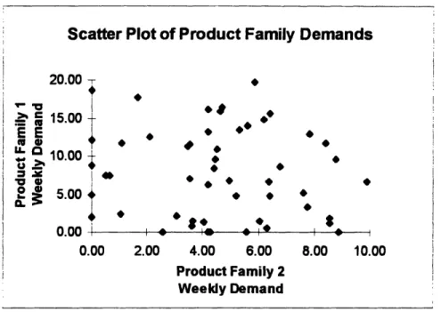
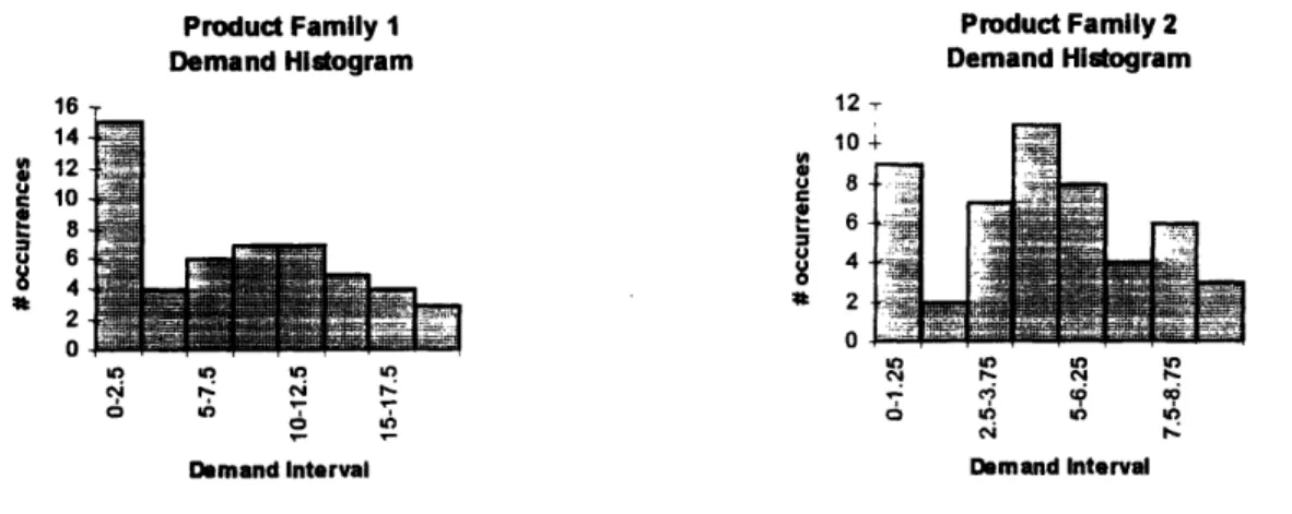
We will specifically consider two product families of photographic media. Product family 1 includes two different formats of slit media (which we will call 1A and 1B) , while product family two has four different formats (labeled 2A, 2B, 2C, 2D). Recall from Section 1.2 that the productfamilies differ primarily in the thickness of paper used in the solvent coating step. And, the product lines within each product family differ only in the

size and shape of the instant film picture. Examination of the past year's demand reveals the following values for the weekly demand distribution:

9IA = 7.78 rolls / week alA = 5.88 rolls / week

9•1B = 0.96 rolls / week oGB = 2.18 rolls / week

Thus, product family 1 total mean demand is given by 9l1 = IlA + LIB = 8.74 rolls / week.

The sum of the product line standard deviations is given by alA + oIB = 8.06 rolls / week.

However, the data for total productfamily demand shows that the standard deviation of total demand is given by aG = 5.45 rolls / week. Thus, we find that the standard deviation of the product family demand is less than the sum of the standard deviations for the individual product lines. Recall from above that this result is expected as long as the product line demands are not perfectly correlated.

Similar analysis for product family 2 results in the following:

P2A = 3.73 rolls / week a2A = 1.82 rolls / week

g2B = 0.88 rolls / week a2B = 1.25 rolls / week

1L2c = 0.24 rolls / week 02c = 0.39 rolls / week

L2D = 0.16 rolls / week a2D = 0.34 rolls / week

Product family 2 total mean demand is t12 = -t2A + P12B + ý2C + 112D = 5.01 rolls per week.

The sum of the product line standard deviations is 0_{2A + G2B + O2C + 72D = 3.8 rolls per}

week. And, the data for total product family demand shows that the standard deviation

of total demand is given by a2 = 2.33 rolls / week. Thus, we once again find that the standard deviation of the product family demand is less than the sum of the standard deviations for the individual product lines.

The above analysis confirms that the magnitude of uncertainty in the demand process for a family of photographic media products is smaller than that of all the individual product lines in the family. Therefore, safety stock held in full web format

(capable of being used to satisfy demand for any one of the product lines in a product family) should be more effective in meeting total product family demand in the event of a production process excursion. Figures 3.1 and 3.2 below illustrate the implementation of a full web inventory policy. In order to pool the variation among product lines in a family, we must hold our safety stock of inventory in a coated, but unslit, full web format. In this manner, we can later slit the safety stock to any format necessary in order to meet the product mix demanded.

Figure 3.1 -Inventory safety stocks held in slit format for each product line.

Figure 3.2 - Inventory safety stocks held in full web format for each product family.

In order to illustrate the benefits a full web inventory policy, we tested the policy against the past year's demand data, and then compared the results to that which would have been obtained by the current, product line specific inventory policy. The current

safety stock policy aims to hold slit material of product lines 1A and 1B which would require a total of 27 full web rolls to generate. Similarly, slit safety stock of product lines