Detection of electric arcs in 42-volt automotive systems

Detection of Electric Arcs in 42-volt Automotive

Systems

by

Joseph Luis

B.S., Electrical Engineering, Massachusetts Institute of Technology (2002)

Submitted to the Department of Electrical Engineering and Computer Science in partial fulfillment of the requirements for the degree of

Master of Engineering in Electrical Engineering and Computer

Science

at the

MASSACHUSETTS INSTITUTE OF TECHNOLOGY

May 21, 2003

©

Author

Department of Ele c and Computer Science

May 21, 2003

Certified by

Markus Zahn Professo of Ele rical Engineering Thesis Supervisor Certified by Dr. Thomas Keim Principal Research-Engineer Thesis Supervisor Accepted by Arthur C. Smith Chairman, Department Committee on Graduate Theses

MASSACHJSJj-# INSTITUTE

OF TECHNOLOGY

I

Detection of Electric Arcs in 42-volt Automotive Systems

by

Joseph Luis

Submitted to the Department of Electrical Engineering and Computer Science on May 21, 2003, in partial fulfillment of the

requirements for the degree of

Master of Engineering in Electrical Engineering and Computer Science

Abstract

The increasing demand of electrical power in today's automobile has led to the research and development of a new 42 V standard. One danger at this new voltage is stable electrical arcing. At the higher voltage, stable electric arcs do not self extinguish and can cause damage to the arcing conductors and cause a fire. This work evaluates possible methods to use to detect and stop electrical arcing before any major damage can occur to the vehicle and more importantly to the passengers. Electronic detection is proposed as the best approach. Arcing current of stable and unstable arcs at -42 V and -14 V are produced by the rebuilt apparatus of a previous MIT experiment that used a motor controlled mechanical switch to periodically energize a conductor to produce stable and unstable arcs. Fourier analysis is performed on the measured current waveforms to look for arc signatures in the frequency domain. Fourier analysis on the average of ten spectra of stable arcs showed that there were no consistent features universally present in stable arcs. Current waveforms of real electrical loads are also measured using electrical accessories (windows,door locks, seat adjustment, lights, sunroof, CD changer, radiator cooling fan) on an electrically operational

1997 Mercury Sable and the amplitudes of their frequency spectra are compared to the

amplitude of the average arcing spectrum. It is determined that although some electrical loads have recognizable shapes in the frequency domain, the amplitudes of the spectra of the loads and the arcs are of the same order. It is concluded that additional research and development is needed for an improved electronic detection approach to detect and identify electric arcs in 42 V automotive systems.

Thesis Supervisor: Markus Zahn

Title: Professor of Electrical Engineering

Thesis Supervisor: Dr. Thomas Keim Title: Principal Research Engineer

Acknowledgements

I would like to start by expressing my gratitude to my supervisors, Professor Markus Zahn and Dr. Thomas Keim, whose expertise, understanding, and patience, added consider-ably to my graduate experience. I would like to thank the MIT/Industry Consortium on Advanced Automotive Electrical/Electronic Components and Systems for giving me the opportunity to work on this project.

Also, I would like to thank Professor George Verghese for taking the time to discuss various aspects of the project. His advice always led to new findings. Alan Wu for explaining the control circuitry of his arcing project and Wayne Ryan for his help in modifying the experimental set-up and bypassing the ignition on the car in the lab.

I appreciate the help of the technical support engineers at National Instruments who spent countless hours on the phone with me to get my LabView code running smoothly.

Finally, I would like to thank my parents who have supported me through all my years at MIT. Without their encouragement I would not have gotten this far and I cannot thank them enough for everything they have done for me.

Contents

2.2.1 The Long Column . . . . 23

2.2.2 Cathode Phenomena . . . . 24

2.2.3 Anode Phenomena . . . . 25

2.3 Voltage and Current M inimums . . . . 26

2.4 V-I Characteristics . . . . 27 3 Detection Methods 29 3.1 Methods . . . . 29 3.1.1 Electronic Detection . . . . 29 3.1.2 Acoustic Detection . . . . 33 3.1.3 Electromagnetic Detection . . . . 36 3.1.4 Optical Detection . . . . 37

3.2 Chosen M ethod: Electronic Detection . . . . 38

3.2.1 Electronic Detection Advantages . . . . 38 -7

3.2.2 Detection using Fourier Analysis . . . . 3.2.3 Localization M ethod . . . . 4 Producing Arcs 4.1 M ain Circuit . . . . 4.2 Control Circuitry . . . . 4.2.1 M otor Control . . . . 4.2.2 Contact Detection . . . . 4.2.3 M OSFET Control . . . . 4.2.4 Noise reduction . . . . 4.3 M easurement Techniques . . . . 4.3.1 Current W aveforms . . . . 4.3.2 Oscilloscope . . . .

4.3.3 Data Acquisition Board . . . .

4.4 Stationary Arcs . . . .

5 Stable Arc Data Analysis

5.1 Arc Event Modelling . . . .

5.1.1 Linear M odel . . . .

5.1.2 Polynomial Model . . . .

5.2 Fourier Analysis . . . .

5.2.1 Full Arc Event . . . .

5.2.2 DC Current Removed . . . .

5.2.3 Effect of Average Arcing Current Magnitude

5.2.4 Zero Centered Arc Transients . . . .

5.2.5 Comparison to DC current . . . .

5.2.6 Effect of Motor Speed on Arc Periodogram

5.2.7 Sine Windowing to Improve Periodogram

5.3 Time Domain Analysis . . . .

on the FFT 8 39 39 41 41 42 43 44 45 46 47 47 48 48 51 53 53 54 57 59 59 63 65 67 72 74 76 77

6 Electric Loads on a Mercury 14V Bus

6.1 Current During Loads . . . .

6.1.1 Ignition Off Mode . . . .

6.1.2 Ignition Accessory Mode . . . .

6.1.3 Ignition Start Mode . . . .

6.2 Fourier Analysis of Load Currents . .

6.2.1 Ignition Off Mode . . . .

6.2.2 Ignition Accessory Mode . . . .

6.2.3 Ignition Start Mode . . . .

7 Arcing on a Mercury 14V bus

7.1 Experim ental Setup . . . .

7.2 A rc C urrent . . . .

7.3 Fourier A nalysis . . . .

8 Conclusions

8.1 Evaluation of the use of Fourier Analysis . . . .

8.2 Suggestions for Future Work . . . .

A LabView Test Control and Measurement Code

A.1 Virtual Instrument Front Panel and Diagram to Control Chopper Motor Test A pparatus . . . . A.2 Virtual Instrument Front Panel to Measure Arcing Current . . . .

B MatLab Analysis Code

B.1 Calculation of the Periodogram of Equations 5.9 and 5.10 . . . . B.2 Polynomial Curve Fitting from Section 5.1.2 . . . .

B.3 Sine Windowing of Section 5.2.7 . . . .

B.4 Analysis of Car Circuit Current from Chapters 6 and 7 . . . .

C Arc Spectrum Figures

9 Contents 81 . . . . 8 1 . . . . 8 1 . . . . 8 2 . . . . 8 2 . . . . 8 3 . . . . 8 5 . . . . 8 7 . . . . 9 0 93 93 94 95 99 99 100 103 103 112 115 115 119 121 123 125

D Ignition Bypass

Bibliography

10

137

List of Figures

2.1 Potential distribution across arcing electrodes where generally Vanode < Vcathode

2.2 Voltage-current characteristics of arcs as a function of gap length for copper

electrodes [15] . . . .

2.3 Stable operating points and extinction point for different load lines on one

V-I characteristic curve of a stable arc . . . .

3.1 Acoustic arc localization using microphones . . . .

3.2 Arc detector and MOSFET placement to locate arc . . . .

4.1 Main circuit of arcing apparatus . . . .

4.2 Main circuit and chopping blade apparatus to create stable arcs .

4.3 Block diagram of complete test apparatus . . . .

4.4 M otor control circuit . . . .

4.5 Contact detection circuit . . . .

4.6 MOSFET control circuit . . . .

4.7 6N137 optoisolator circuit . . . .

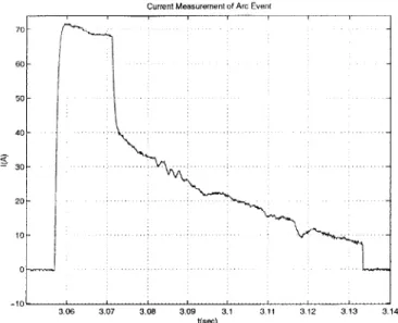
4.8 Current waveform measured from arcing apparatus . . . .

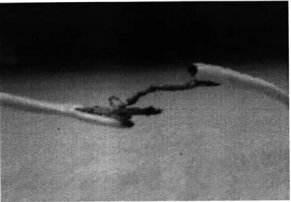
4.9 Damage caused to wire from periodic arcing . . . .

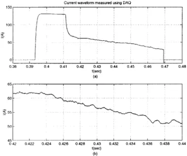
4.10 Current measured using oscilloscope (a) full test event (b) zoomed in when arc is on to show 8 bit, ~-'400mA sampling step in amplitude at 200 kHz sam pling rate . . . . 4.11 Current measured using DAQ showing 15 bit sampling (-3mA steps) (a) full test event (b) zoomed in when arc is on . . . .

5.1 Square pulse to model DC current . . . .

5.2 Line from -T 2 to T2 to model current falls . . . .

5.3 M odel of arc event . . . .

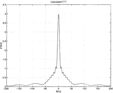
5.4 Calculated FFT magnitude of one arc model . . . .

11 23 28 28 . . . . 35 . . . . 40 . . . . 41 . . . . 43 . . . . 44 . . . . 44 . . . . 45 . . . . 46 . . . . 47 . . . . 48 49 50 50 54 54 55 58

5.5 Current (a) measured during arcing current and (b) the 3rd order

approxi-mating polynomial model . . . . 58

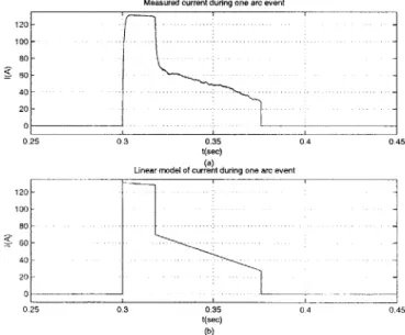
5.6 Current (a) measured during a full arc event and (b) its approximating linear model ... ... ... 59

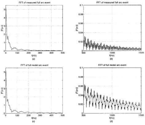
5.7 FFT magnitude of (a)&(b)current measured during a full arc event and (c)&(d) of its linear model for the waveform in Figure ?? . . . . 60

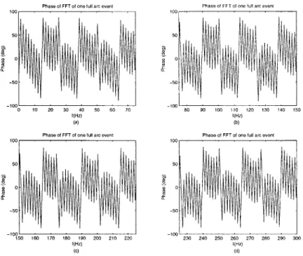
5.8 Phase of the full measured arc event in Figure 5.6 from zero to 300 Hz . . . 61

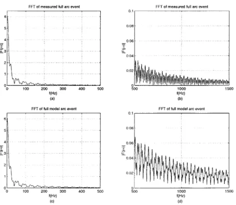
5.9 Current (a)measured during a second full arc event and (b)its approximating linear m odel . . . . 62

5.10 FFT magnitude of (a)&(b) current measured during a second full arc event and (c)&(d) of its linear model for the waveform in Figure 5.9 . . . . 62

5.11 (a) An arc event with DC current step removed and (b) its approximating polynom ial m odel . . . . 63

5.12 FFT of (a)-(b) one arc event with DC current step removed and (c)-(d)FFT of its polynomial model . . . . 64

5.13 (a) Linear arc model with 10 A peak to peak noise added and (b) its FFT 64 5.14 (a) Linear arc model with 2 A peak to peak noise added and (b) its FFT 65 5.15 (a) Linear arc model with 1 A peak to peak noise added and (b) its FFT 66 5.16 (a) One arc event and (b) its 3rd order polynomial model . . . . 68

5.17 Arc event from Figure 5.16 (a) with its polynomial model subtracted out . 68 5.18 Zero centered arc transients 1 through 5 used in the average periodogram analysis . . . . 69

5.19 Zero centered arc transients 6 through 10 used in the average periodogram analysis . . . . 70

5.20 Periodogram of one arc event transient . . . . 71

5.21 Average of 10 arc event periodograms . . . . 71

5.22 Zero centered DC current and arcing transients . . . . 72

5.23 Periodograms of DC and arcing transients over the frequency range of zero to 4 kHz. The DC transient periodogram is multiplied by 10 to be viewable on the same scale as the arc transient periodogram . . . . 73

5.24 Full arc event with the chopping motor at twice the speed (2 contacts/second) 74 5.25 Waveform of (a) measured arc from Figure 5.24 with DC step ignored and (b) its model with the motor at twice the speed (2 contacts/second) . . . . 75

List of Figures

5.26 Periodogram of one arc transient with the motor operated at twice the speed

from zero to 3 kH z . . . . 75

5.27 Average periodogram over 10 arc events with the motor at twice the speed 76

5.28 Effect of sinusoidal windowing on arc transient data of Figure 5.18 arc #1 77

5.29 Average over 10 periodograms of windowed arc transients . . . . 78

6.1 Current during turn-on operation of (a) door locks (b) parking lights (c) CD

changer (d) seat tilt . . . . 82

6.2 Current during turn-on operation of (a) windows (b) sunroof (c) windshield

w ip ers . . . . 83

6.3 Turn-on current waveform during ignition start mode of radiator fan and

dashboard lights . . . . 84

6.4 Periodogram of measured door lock transient from Figure 6.1(a) over the

frequency range of zero to 3 kHz . . . . 84

6.5 Periodogram of measured parking lights transient from Figure 6.1(b) over

the frequency range of zero to 3 kHz . . . . 85

6.6 Periodogram of measured CD changer waveform from Figure 6.1(c) over the

frequency range of zero to 3 kHz . . . . 86

6.7 Periodogram of measured seat tilt waveform from Figure 6.1(d) over the

frequency range of zero to 3 kHz . . . . 87

6.8 Periodogram of measured power window waveform from Figure 6.2(a) over

the frequency range of zero to 3 kHz . . . . 88

6.9 Periodogram of measured sunroof waveform from Figure 6.2(b) over the

fre-quency range of zero to 3 kHz . . . . 88

6.10 Periodogram of measured windshield wipers waveform from Figure 6.2(c)

over the frequency range of zero to 3 kHz . . . . 89

6.11 Periodogram of measured ignition start waveform from Figure 6.3 over the

frequency range of zero to 3 kHz . . . . 90

7.1 Experimental setup for creating 14 V parallel arcs in the engine compartment

of the M ercury Sable . . . . 94

7.2 (a) Current waveform during one 14 V arc event (b) zoomed in near 14 V

arc and current turn off . . . . 95

7.3 Current measured during headlight operation and one parallel arc event . . 96

7.4 Periodogram of headlight operation and one arc event of Figure 7.3 showing

little different between normal and arcing operation . . . . 96

D.1 Ignition key cylinder before bypass . . . . 137 D.2 Ignition key cylinder after drilling . . . . 137

List of Tables

2.1 Vm and Im for different cathode and anode materials [2] . . . .

Arc Model Constant Definitions . . . . Arc Model Constant Values . . . . Variances of 10 Arc Events: Motor Speed at 1 contact/second . . . . . A.1 Operating Range and values used in tests for variables on test controls VI . A.2 Values used in tests for variables on measurement controls VI . . . .

26 56 57 79 103 112 15 5.1 5.2 5.3

Chapter 1

Introduction

Today's automobile is more luxurious and contains more electrical components than ever before. Consequently, the power demands of the automobile are rapidly increasing. A variety of systems including anti-lock brakes, power windows, seat warmers, as well as stereo and navigation systems all require electrical power that was not needed in older vehicles. It has been predicted that by the year 2005, electrical components will demand an average power above 2kW [1]. In 1994, Mercedez Benz and MIT, along with seven other companies, met to develop a higher voltage bus. A 42 V bus was recommended. The MIT/Industry Consortium on Advanced Automotive Electrical/Electronic Systems, which is comprised of researchers at MIT as well as companies from the automotive industry, was formed soon after to investigate the switch to the higher voltage.

1.1

Arcing in a 42 V System

One potentially dangerous issue with the new 42 V bus is electric arcing. In the present 14 V system, current interruptions result in unstable arcs. However, if the voltage source were made high enough(greater than 15 V), a stable discharge would be produced [2]. The large amount of energy in the stable arcs as well as the extremely high temperatures reached can burn wire insulation as well as start fires. On automotive systems, melting insulation and fire can ignite fuel vapors, posing a threat to the passengers.

Arcing can occur anywhere on the wire harness. If the insulation of a wire becomes worn, for example from aging or damage during vehicle maintenance, so that an exposed wire makes contact with the chassis of the car, a parallel arc can occur. In effect, a short circuit is created between the two battery terminals resulting in a high current stable arc. If a wire is cut or if electric contacts separate, a stable series arc can occur. Circuit current is limited by the loads on the car but the high temperatures of the are and the large amount of energy can still cause fire.

Fuses are presently used to protect the system in overcurrent situations. However, there is a possibility of creating high current stable but intermittent arcs that do not clear the

-fuse because the RMS current is below the -fuse rating. For example, if a car is on a bumpy road, a damaged wire may make repetitive contact with the chassis. This could create a stable arc during each contact separation but keep the RMS current low enough that the fuse protecting the circuit does not clear. This is a worst case scenario since instantaneous currents are high and the temperature of each arc causes damage to the insulation and melting of the contact materials.

Because of the danger of stable arcing in the 42 V bus, new connectors and other products that are less prone to stable arcing have been developed. Currently, no method exists that can prevent all stable arcs in electrical systems prone to stable arcing. Because of this, a detection method must be developed that can minimize the damage caused by stable arcing. This work focuses on the development of a detection method for arcs in the 42 V automotive system.

1.2

Previous Work

1.2.1 Arcing Energy

The importance of arcing at 42 V was first brought to the attention of the MIT/Industry Consortium by Yazaki Inc. A mechanical chopper was used to make periodic contact with a test wire. On separation, the contacts would create an arc. Battery voltages of 12 V and 36 V were used in the tests and the arcing created was compared. Results were dramatic. Arcing with a 36 V battery source created arcs that burned wire insulation, melted the test wire, and destroyed the blade used to make contact with the test wire. By contrast, arcs at 12 V did much less damage to the contacts.

Further work was done at MIT by extending Yazaki's experiment. A fuse was included in the test circuit and computer control of circuit current duration during contact showed that incidents of periodic arcing that did not clear the fuse could indeed occur [3]. Tests using 12 V and 36 V sources were performed and it was found that arcing energy was 10 to 100 times greater in the case of a 36 V source. Molten copper and steel from the contacts was seen only in the 36 V case, showing the possible dangers of an unprotected 42 V system. Arcing that did not clear the fuse was generally less intense than the arcs produced by the Yazaki work.

1.2 Previous Work

1.2.2

Arc Detection

A variety of work has been performed in the field of electric arc detection and is reviewed

in detail in Chapter 3. The majority of this detection work has been done in 60 or 50 Hz

AC systems and a lesser amount in DC systems.

Such research has been performed by B.D. Russell and his group at Texas A&M University in the detection of arc faults on power distribution feeders. They studied the changes in energy from cycle to cycle on the AC line of various frequency harmonics [4, 5, 6]. These changes in energy between cycles has enabled them to develop algorithms to detect arc faults in AC power systems. Another method of detecting arcs in AC systems was developed at the University of Manitoba in which the asymmetry between the current magnitudes of the positive and negative half cycles of the current are compared in order to determine that a fault is occurring [7].

Arc detection has been performed by detecting arc acoustic, electromagnetic, light, and heat radiation as well. At Schneider Electric Industries, work has been performed in AC systems in which the acoustic emission of a series arc is measured and characterized [8]. Thresholds of sound amplitude and sound duration are used to monitor sound on the busbar

and determine when an arc occurs. The power systems research group at the University of Saskatchewan has combined acoustic, electromagnetic, and infrared radiation to produce

a more reliable AC arc detection algorithm and to locate where an arc is occurring

[91.

The detection of arcing faults by electromagnetic detection has also been performed at the University of Bath where electromagnetic radiation is used to detect and locate arc faults in AC power systems [10].

For detecting arcs in switch gear, busbar, and circuit breaker cubicle systems, The ABB Group has developed a product called the Arc Guard System. Using optical detectors and fiber optics, the Arc Guard System detects large changes in light intensity due to arcing and trips the breaker.

More relevant to automotive applications is arc detection work that has been performed

in DC systems, specifically in the telecommunications 48 V DC power system. Research

at Bell Communications Research has led to the detection of electric arcs by analyzing the frequency spectrum of the arc current and of normal current operation of the system

[11, 12]. This spectrum analysis looks promising as the tested 48 V DC telecommunication

system is similar to the proposed 42 V DC. Additional work has also been performed at Hendry Telephone Products in which the spectrum of the current is analyzed by the arc's fractal nature in order to develop proper filters and algorithms to detect arcing in the 48 V

DC system [13]. Although slightly more complex, this may be a reasonable future approach

to take for the 42 V automotive system.

1.3

Thesis Scope

The goal of this research is to select and investigate a method of arc detection for use in the new 42 V automotive system. An evaluation of various detection methods and their feasibility in automotive systems is carried out. An electrical method of detection is selected because of its possible advantages in cost and in simplicity. Time and frequency domain analysis of circuit current during arcing events and normal operation is then performed. From the thesis research we conclude that Fourier analysis as well as energy monitoring may not be accurate enough for detecting and identifying arcs in 42 V automotive systems as arc current and normal operation curent have similar frequency spectra. Comparisons are made to previous work in DC systems which have successfully accomplished detection through Fourier analysis to determine the cause of our inability to produce similar results.

1.4

Thesis Organization

An overview of electric arc theory is presented in the following chapter. A discussion of detection methods researched in previous work and their comparisons follows in Chapter 3. An experimental setup that produces 42 V arcs is described in Chapter 4 and analysis of the data is then presented in Chapter 5. Measured circuit current during normal operation and during 14 V arcing on an electrically operational vehicle is presented and analyzed in Chapters 6 and 7. Conclusions and suggestions for future work follow in Chapter 8.

Chapter 2

Arc Physics

Before attempting to detect an arc, we should first understand the physics of arc discharges. Arc discharges can occur in many ways including electrical breakdown of gas between elec-trodes and by the separation of current-carrying electric contacts. The voltages in the new 42 V automotive system will not be great enough to cause breakdown of air and arc discharges will occur by the drawing apart of current carrying conductors. The following sections describe are formation and arc characteristics of stable arcs that can occur in a 42 V system.

2.1

Arc Formation

Arcing at the new higher voltage will occur by the separation of energized conductors, creating either a series or a parallel arc. In a series arc, current-carrying electrodes separate, forming a stable arc. The electric load in series with the arcing wire limits the current. In parallel arcs, a current-carrying electrode is grounded, as can happen if a damaged wire touches the grounded chassis, and separation from the grounded electrode forms a parallel arc whose current is limited by the impedance of the chassis and the source.

As the electrodes separate, the surface area of contact becomes smaller. The current flowing in the circuit must then flow through the smaller area of much larger resistance and the current density at the electrodes increases. When the electrodes are near separation, the

contact area is so small that the 12R heating is enough to melt the electrode metals and

a liquid metal bridge forms [14]. If the contacts continue to separate, the liquid bridge ruptures explosively. The rupturing is due to boiling at the hottest part of the bridge or because of insufficient surface tension forces in the system to maintain a stable liquid bridge of that length.

After rupture of the liquid bridge, the formation of a stable arc depends on the circuit char-acteristics, conductor material, as well as the speed at which the conductors are separating. If conditions are met for a stable arc to occur, a short arc follows [2, 14]. The short arc

forms when the electrodes are at a distance of approximately 10 4 cm and lasts on the order

of lys. During this time, electrons fall freely between the cathode and the anode electrodes and rarely make any collisions because the distance between the cathode and the anode are on the order of the electronic mean free path [14]. At this point, the circuit current through the arcing electrodes is dominated by electrons emitted from the cathode that then hit the anode with the energy acquired in the transition from cathode to anode. Because the anode is receiving the majority of the energy of the arc during the short arc, the anode material evaporates at a faster rate. In systems of higher voltage, typically 400 V, the material from the cathode evaporates more quickly because of the Joule heating creating small points on the cathode that boil away [14]. However, in the case of the new automotive voltage, short arcs will be of the "anode" type, in which during short arcing the evaporation of electrode material comes mainly from the anode.

As the electrodes continue to separate, a transition from the short arc to the "long" column is made. Because the separation distance between the electrodes are no longer on the order of the electronic mean free path, electrons cannot freely fall from the cathode to the anode as in the short arc. Collisions now occur during the travel of electrons from the cathode to anode and cathode and anode fall regions develop as described in Section 2.2. The large amount of energy in the stable arc continues to cause damage to the electrodes. If the separation distance of the electrodes continues, the voltage required to sustain the stable arc increases and if the distance of the electrodes becomes large enough the arc will extinguish. If the electrodes stop moving and the stable arc is allowed to persist, the arc will continue until the electrode material is completely evaporated or the energy in the source falls below that necessary to maintain stable arcing conditions.

If the arcing electrodes once again contact each other after arcing, we have a periodic arcing condition. In a car, movement over bumps could cause arcing wires to make repetitive contact. Electrodes under these arcing conditions repeat the process of the rupturing of a liquid metal bridge, a short arc, and the formation of a stable long column. Because of this, major damage can be caused by periodic arcing. The extent of the damage depends on the source voltage and electrode materials. For example, on the 14 V bus, a short arc forms but a stable long column does not form. Periodic contact thus causes minor, if any, damage to the electrodes. At 42 V however, the stable long columns created by separating electrodes can cause major damage to electrodes.

2.2

Arc Regions

When the long column of a stable arc forms, current must be carried by the gas between the electrodes. For this to happen, the gas must become conducting by having charged

2.2 Arc Regions

carriers either created in the gas or injected from the electrodes. At each of the electrodes there must also be a transition of the circuit current from the electrodes to the gas. This creates three main regions, the cathode fall, anode fall, and the long column with an electric

potential distribution shown in Figure 2.1. The electrode column junction regions are

particularly complex because of the necessary transitions of current from metal electrode to gas. Properties of each region are further described in the following sections.

V Vanode Vcolumn _Varc Vcathode x Gap Length

Figure 2.1: Potential distribution across arcing electrodes where generally Vanode < Vwathode

2.2.1 The Long Column

The arc consists of a quasi-neutral column of ionized gas containing electrons and negative and positive ions [14]. The literature pays particular attention to the electrons and positive ions, neglecting negative ions. Positive ions are formed in the gas by ionizing collisions with electrons or are injected into the column by the anode. This results in a high temperature arc and equilibrium is achieved when the rate of charge generation is balanced by the rate of recombination. The quasi-neutral arrangement of the charges in the charged gas are known as a plasma with the number density and charge per carrier of electrons and positive ions being respectively (ne, -e) and (ni, qi). Quasi-neutrality requires that

-ene + qin ~_ 0 (2.1)

where e = 1.6 x 10-19 Coulombs is the charge on an electron. The arc current is then

related to the product of the each charge carrier's charge density and its respective velocity by

Jtotal = -neebe + niqihi (2.2)

where Ve is the drift velocity of electrons, and Nj is the drift velocity of the positive ions. Because the mass of the positive ions is large compared to the mass of the electrons, Ve

is much larger than iij. This shows that the current in the column is carried primarily by

electrons and that the positive ions serve mainly to keep the region in a quasi-neutral state.

The fraction

f

P, and ionization potential Vi in volts is given by Saha's equation shown in Equation 2.3

where k is Boltzmann's constant [2, 14].

(

In summary, in a stable arc the column is a quasi-neutral region in which the current is carried primarily by electrons. The region is at an extremely high temperature and is in thermal and charge equilibrium.

2.2.2 Cathode Phenomena

At the cathode there exists a drop in potential known as the cathode fall and is shown in Figure 2.1 as Veathode. Generally, the cathode fall is on the order of 10 V and is due to current flowing across the electrical-plasma interface and depends on the electrode material [14]. At the cathode, electrons are extracted and accelerated across a high electric field region into the positive column where they either ionize neutral particles or recombine with positive ions.

2.2 Arc Regions

Electrons can be extracted in several ways. One way is the emission of electrons as a

consequence of positive ions impinging on the cathode surface. However, this method is unlikely to be the main source of electrons since a cathode fall of hundreds of volts would be required to maintain a glow discharge [141.

Another method by which electrons can be emitted is thermionic emission from a hot enough cathode if emission is obtainable at temperatures below the boiling point of the cathode material [14]. The temperature at the cathode can be kept high by the energy received at the cathode from positive ions accelerated in the cathode fall.

Strong electric fields on the order of 107 V/cm at the cathode surface can also yield high

electron emissions. If the current density at the cathode is large enough, a field of this magnitude can be produced by the space charge created by the incoming positive ions. If thin insulating layers are created at the surface of the cathode, positive ions can collect on this layer and also create high electric field strengths capable of pulling out electrons from the cathode.

Thus, there are a variety of ways in which electrons can be emitted to create the cathode fall region. One or more of the above mechanisms are present in arcing electrodes and exactly which mechanisms are occurring are difficult to specify.

2.2.3 Anode Phenomena

The conductor receiving electrons from the cathode is the anode. Except in special cases, the anode does not emit positive ions and the current carried at the anode is carried solely by electrons [2, 14]. Because of this, there will be a small region of negative space charge directly in front of the anode electrode and a potential fall Vanode is created. Unlike the cathode, both charge carriers are not produced in the anode region. In the cathode, electrons are emitted at the negative electrode surface and electrons and positive ions are produced at the column end of the cathode fall. However, at the anode, only positive ions are formed, making the anode potential fall smaller than the cathode fall.

Another difference at the anode is that the energy required to produce charge carriers is

much less than at the cathode [141. This is due to the fact that the anode current is

carried by electrons and no positive ions enter the anode. If we look at the total arc current I = 1,

+

an l[c due to positive ions flowing in the opposite direction. However, in the anode region,

there only exists a current 1ea due to electrons. Thus,

9-

produced per second in the anode, compared to that must be produced in the cathode.

-Since 1e >> Ij, there is less energy required to produce charge carriers in the anode [14].

2.3

Voltage and Current Minimums

In order to sustain a stable arc, the arc voltage must be greater than the minimum arc

voltage Vm and the arc current must be greater than the minimum arc current I. Minimum

stable arc voltages and currents for various electrode materials are shown in Table 2.1. The

Table 2.1: Vm and Im for different cathode and anode materials [2]

Material VM(V) Im(A) (cathode) (anode) Sb 10.5 -Zn 10.5 0.1 Ag 12 0.4 Cu 13 0.43 Bronze 13.5 0.31 Sn 13.5 -Al 14 -Ni 14 0.4 Au 15 -Steel 15 0.5 Pt 17.5 -Carbon 20 0.03

minimum arc voltage Vm primarily depends on the cathode material due to the cathode potential fall dominating the arc voltage. The cathode fall depends on how easily electrons are emitted into the plasma column and this is a function of the cathode material. Notice that the voltage minimums required to sustain a stable arc are all lower than the new 42 V system.

The minimum arc current Im is mainly a function of the anode material

[2].

shown in Table 2.1, Im is less than 1 A. As will be shown in Chapter 4, creating arcs using

3 12 V batteries results in current on the order of 100 A, much greater than Im. Chapter 7 shows arcing on a 14 V system and although the current is around 45 A, the voltage of one battery is insufficient to sustain a stable arc.

2.4 V-I Characteristics

2.4

V-I Characteristics

Vm and 1m create asymptotes by which we can begin to draw the VI characteristics of stable

arcs. The shortest possible arc does not follow these straight asymptotes, however. Instead

the shortest possible arc obeys Equation 2.4

(V - Vm)(I - IM) = C (2.4)

where C is a constant that depends on the material of the electrodes [2]. Thus the shortest

possible arc follows a hyperbola. If the distance between the electrodes increases, the

voltage-current characteristics change but continue to be related by hyperbola functions and obey the relationship

[V - Vm - Varc(d, I)](I - Im) = C(d) (2.5)

where Varc(d, I) is the arc voltage as a function of gap length d and circuit current I and

C(d) is a constant that depends on the material of the electrodes as well as the gap length

[2].

Figure 2.2 shows how the the voltage-current characteristics vary as a function of electrode gap length. Each curve represents the voltage and current relationship for a stationary stable arc for copper electrodes at a particular gap distance. To determine if a stable arc

exists, a load line can be drawn with intercept Vbatt on the voltage axis and Vlat on the

current axis where R is the circuit resistance. Intersection of the load line with the voltage-current curves gives points at which an arc can exist. The stable operating point is the point of greater current and lower voltage. This can be explained by noting that if the arc is at the point of large voltage and smaller current, there is more voltage than is needed to maintain a stable arc. The arc will thus heat up, lowering the arc resistance, and the current will increase until the second operating point is reached [15].

If the gap length is slowly increased, the stable operating point moves along the load line in the direction of decreasing current, and increasing arc voltage. When the load line is tangent to the hyperbolic curve the arc extinction length has been reached and any further increase in gap distance will extinguish the arc. Figure 2.3 shows two load lines intersecting one V-I

characteristic curve of an arc. One load line intersects at two points and has a single stable operating point. The second is tangent to the V-I curve and is at the extinction point. For this load line, if the gap length is increased any further, the arc will extinguish because the V-I curve for the larger gap length will no longer intersect the load line.

V Uarc3 20 10

t300

Figure 2.2: Voltage-current characteristics of arcs as a function of gap length for copper electrodes [15] V) Load lines Extinction point Stable operating point

Figure 2.3: Stable operating points and extinction point for different load lines on one V-I characteristic curve of a stable arc

-Chapter 3

Detection Methods

It would be desirable to be able to detect an arc event before it occurs. However, such a method does not exist yet. The next approach is to detect that an arc is beginning to occur as reliably and as fast as possible. This thesis work takes the approach of minimizing any possible damage and danger caused by the are as quickly and as accurately as possible when analyzing detection methods. In this chapter we examine various possible techniques of arc detection for automotive applications.

3.1

Methods

There are a variety of ways to detect arcing once such an event is occurring. Detectors for power distribution feeders have been developed that monitor circuit currents as well as radiated energy in the form of sound, electromagnetic waves, and light during electric arcs. The methods analyzed here have been used either in real applications or in the laboratory. One important consideration in what method to use for detection is how the arc will be localized. Once the arc is detected, it is necessary to determine the circuit in which the arc is occurring and to turn the current off. For this reason, a method of localization under each detection technique is also analyzed.

3.1.1 Electronic Detection

Electronic detection uses techniques that monitor specific circuit current and voltage changes during an arc event. For real world applications, voltages across the arc may not be a rea-sonable approach given the uncertainty of the location of the arc fault. Circuit current changes during an arc are therefore a more widely used method of detecting electric arcs. Depending on the system, a variety of approaches can be used.

AC Systems

-In AC systems, arc detection can be performed in different ways, all using the fact that the current has positive and negative half cycles. One approach by a group at Texas A&M University was to monitor the change in energy of the current signal [4]. Using the sum of squares of the sampled data they obtained the energy of the signal. Comparing the energy in one cycle to the previous cycle allowed them to characterize the change in energy that an arc produces per AC cycle. This method distinguished steady AC operation from fast transients seen when capacitor banks switch on and off as well as the operation of air switches. Furthermore, filtering the time domain waveform before performing energy calculations using bandpass filters with center frequencies at 180 and 210 Hz yielded vast improvements in the detection of arcing faults. In the filtered waveforms, energy would change by close to a factor of 50 during arcing compared to a factor of 6 in the unfiltered case.

A dynamic threshold was determined as the average energy per cycle and any energy varia-tion over the threshold could take on two possible states, an "event" or an arc fault. If the energy in one current cycle was 25% greater than the previous cycle, the amount of time of that change in energy would be calculated. Further fluctuations in the signal energy by 75% over three cycles would classify as an event. Once again, fluctuations in energy are calculated and if they continue, a fault is said to have occurred. Sensitivity of the detector could be changed by varying the number of cycles over which changes in energy must occur to be classified as events or faults. This algorithm works well because the arcing faults have much longer time durations compared to the time durations of capacitor banks switching on and off. This method would be difficult to implement in the new automotive system given that we must work in a DC system in which we cannot compare current and energy during different cycles. The AC zero crossing of the current can create recurring arcs which create detectable changes in energy while in a DC system recurring arcs will only occur during periodic arcing in which the electrodes make intermittent contact. It is a possible method of detection but not one generally applicable to DC automotive systems.

An improved method used at Texas A&M University was to monitor the content of the harmonics and in-between harmonics of the fundamental line frequency as a function of

time [5, 6]. The in-between harmonic frequencies are defined as the frequencies midway

between the harmonics. So for a 60 Hz line, some in-between harmonics would be 90, 150, and 210 Hz. The input signal from the monitored 60 Hz line current is filtered by a number of band pass filters whose center frequencies are either the harmonics of the line, or the between harmonics. The energy changes per cycle are calculated for various in-between harmonic frequencies. As with their previous work, changes in energy in the filtered signals beyond a specified amount of the dynamic threshold will set the detector to begin calculations to determine whether a fault is occurring. By comparing many odd harmonics and in-between harmonics, -180% of arc faults are detected. However, as the authors state,

-3.1 Methods

the arcing faults detected were created and controlled and the same detection rate may not apply to real world applications.

The possibilities of using this method in the automotive system are few. We cannot compare the current and energy during different cycles because we are working with a DC system. It may be possible to choose a specified amount of time to monitor but the energy changes would not be the same as in the AC system due to the recurring energy faults caused by the zero crossing of the current. Also, one assumption made is that any transients from switching operations occur in a time on the order of a few cycles or less while arcing will occur over many more cycles. As we will see in Chapter 6, this is not always true of

transients in the automotive system.

A different approach to the AC system arc detection problem is to use the asymmetry

caused in the waveform by arcing [7]. Two terms are defined, current flicker and

half-cycle asymmetry. Current flicker is defined as the difference between the magnitude of the positive current peak from one cycle to the next. This is also done for the negative half cycles. Half-cycle asymmetry is determined by first finding the difference between the peak magnitudes of two successive half cycles. The calculation window moves over by half a cycle, making the previous second cycle the first cycle of the new calculation. The same difference is calculated between half cycles. An overall difference between the two calculations is then determined. These calculations are made based on observations that the fault current magnitude can vary greatly from one cycle to the next and that either the negative or positive half cycle current peak magnitudes are larger. After the calculation of the current flicker and asymmetry, a score is given to any transient based on the values it produces for flicker and asymmetry. Loads such as fluorescent lights, short circuits, and a computer are added to the system and the flicker and asymmetry of the transients they produce are calculated. Flicker and asymmetry are calculated for various arc faults as well and because the flicker and asymmetry are higher in arc faults, a threshold can be determined. An arc welder was used as well and it was determined that the detector could not differentiate an arc fault from the arcing load.

Because the current flicker and asymmetry method relies heavily on how the AC current peaks vary, this method cannot be used for the automotive DC system. Monitoring the variance of the changes of the current in time might be one approach and the possibility of using this method is explored in Chapter 5.

DC Systems

We now shift our focus to DC systems. One possible approach that has been used in the

telecommunications industry's 48 V DC system is to monitor the frequency spectrum of

the circuit current. Work performed at Bell Communications has shown that in their 48V system, a threshold of the amplitude of the frequency spectrum can be found to distinguish arcing from normal operation current [11, 12]. Noise current on the DC system was studied and the spectrum of the noise was compared to that of the arc. Noise current was defined as any current that was not DC. It was found that the noise spectrum differed enough from the arc spectrum in amplitude at practically all frequencies. A detector was made that monitored the circuit current and if the amplitude of the calculated spectrum was above a threshold, an arc was considered to be occurring.

This approach looks very promising for the new 42 V DC automotive system. The ability to perform this task in a 48 V system shows that there is a possibility of doing the same in the 42 V system. What may be a difficult task in the automotive system is that the normal operation DC current level varies. Some electrical loads require more current than others, and if they are used in combination, the DC level is different. For this, a dynamic threshold can perhaps be used as in the work by Russell's group. In effect, we would recognize a DC level, ignore it, and only pay attention to the variations which occur around the DC signal. One particular difficulty with using the method used at Bell Communications, as will be seen in Chapter 6, is that the noise current spectrum in an automotive system is not substantially lower than the arc current spectrum for all cases. In fact, some electrical loads can produce noise transients which are greater in amplitude at some frequencies than in the arcing spectrum.

Another approach for detecting arcs in DC telecommunications systems was taken by a group at Hendry Telephone Products [13]. The arc spectrum is first seen as being fractal in nature. The current is monitored by a current probe and is bandpass filtered at an un-specified frequency. The signal is then passed through a non-linear process which produces an intermodulation of the components of the input spectrum and its output is filtered by a sharp bandpass filter with a center frequency much lower than then initial bandpass filter. The amplitude of the output is determined by the amplitude of the initial input as well as the number of frequency differences produced by the non-linear process meeting the re-quirement of the center frequency of the second bandpass filter. A detection circuit is then used to determine if the output of the second bandpass filter is constant. Because arcing current is chaotic, the input to the detection circuit must not be constant in order to be considered an arc. Third and fourth bandpass filters are used to determine a "chaos level" and the overall output is checked against a set sensitivity level.

The approach taken by Hendry Telephone Products appears to work well. As we will see in Chapter 5, the spectrum of the arc at ~42 V, and at 48 V as shown by Hendry Telephone Products, contains a continuous range of frequencies and this fact is used in this detection

-3.1 Methods

method by using the non-linear process and sharp bandpass filter. In this research however, we will focus on trying to use simpler methods first before attempting to use more complex method such as this.

Arc Localization

Electronic localization of an arc can be performed in at least two ways. In an automobile, various electrical components are grouped together and protected from over current condi-tions by a fuse. If the fuse clears, operation of the components protected by that fuse is lost. We can thus incorporate a detector into each of these fused circuits. If any of the detectors determine that an arc is present, the detector's particular circuit is opened to protect the components from major damage.

In the automobile industry, cost is a major factor. Automotive circuits today are protected by far too many fuses to make using a detector in each fused circuit cost effective. We can use only one detector if we place it in the main circuit of the vehicle. Circuit current variations due to an arc will also be seen in the main circuit and determining that an arc is present will not be affected. However, using one detector requires us to develop a method to determine which fuse-protected circuit must be turned off. The arcing circuit can be determined by sampling the current in each fused circuit. In the case of many fused circuits, a method for the order of sampling must also be developed.

3.1.2 Acoustic Detection

When an arc occurs, a sound is emitted by the event. If we can differentiate between other sounds in the system and in the environment of operation, we can detect the arc event. Microphones and transducers can be placed throughout the vehicle to monitor vehicle sound. Noise which may interfere with the arc signature can be characterized and filtered or ignored by other means.

Acoustic emission in AC low voltage distribution switchboards has been characterized and

detected using ultrasonic sensors by a group at Schneider Electric Industries [81. Ultrasonic

signals measured during an arc are measured and it can be seen that the time domain waveform has three distinguishing features. The first is a high change in signal energy. It was also seen that the arc signal consisted of a lower but sustained energy in subsequent cycles. This energy was also modulated by the 50 Hz line frequency.

Three tests were performed on the data. The first was a test which compared the energy in

k samples of one cycle with a threshold. If the energy of the k samples was greater than the

-threshold, a second test would be performed. The second test compared the peak energy of the present cycle with the average energy in the next cycle. Because during arcing, there was a large contrast between the first energy burst and subsequent energy, this allowed the detector to ignore noise such as mechanical shock to the busbar that did not exhibit type of energy behavior. The final test checked for energy modulation. The test gave a positive result if a local maximum between 90 and 110 Hz existed and if that maximum was greater than 50% of a given global maximum. The tests were performed on the rectified 50 Hz signal. This produced 100 Hz time signals and because of this, the test looked for maximums between 90 and 110 Hz.

This particular acoustic detection method would be difficult to implement in automotive systems. Because there is no fundamental frequency in the DC system, we will not see the characteristic energy modulation seen in the above work. In addition, transducers placed on the cars chassis to measure ultrasonic noise would be subject to an enormous amount of mechanical vibration signals from engine and road noise and vibration. Just the operation of the vehicle in different road conditions and at different speeds would change the characteristics of the vibrations. This would make it extremely difficult to detect an arc using this method.

One difficulty that can arise in acoustic detection is how to differentiate between direct and reflected sound due to their arrival time differences at acoustic inputs. One solution is to use a pressure zone microphone (PZM) in which a microphone combined with a boundary plate are used to create an input in which the direct and reflected sound add in phase as was done at the University of Saskatchewan [9]. The microphone used had a sensitivity of -74dB and a frequency response from 20 to 18000 Hz. The sound at the microphone shows a sharp peak when an arc begins, followed by exponential decay. Higher frequency content rides on top of the signal. Pattern recognition techniques using neural-networks were used to create a stored pattern of an arc's sound time domain shape.

Success was shown with this method of acoustic detection. However, this acoustic detection method was one of three different methods used in parallel with two other methods in order to obtain high reliability. Combined with electromagnetic and infrared detection, the overall detector was reliable. In combination, a false trip from one detector would not necessarily mean a false trip from the combination of detectors. Using three detection methods increases cost and we would like to avoid that for the automotive system. If the acoustic detection method alone is prone to false alarms then it may not be the most adequate means of arc detection in automotive applications. Another issue in acoustic detection is that the combined directivity of the microphones would have to cover every part of the car. Because the microphones are not omnidirectional, this can quickly become a difficult problem to solve in the complex frame of a vehicle.

3.1 Methods

Locating the arc can be achieved using the fact that sound radiated by the arc will arrive at the microphones at different times [9]. This is illustrated in Figure 3.1. Using arrival time

(13 (11

Arc M

d3 d,

Figure 3.1: Acoustic arc localization using microphones

differences of the arc emitted sound at microphones M1, M2, and M3, distances di, d2, and

d3 can be calculated and a location of the arc determined. For example, we know that the

distance travelled to each microphone is d, = vt, where t, is the time it takes the arc sound to reach the nth microphone. By Equation 3.1, where n and m are integers representing the number of the microphone, we can find the difference between the distances travelled between any of the microphones and find the distances to the arc for each microphone. The more microphones used in the localization calculation, the more accurate the result would be.

v(t, - tm) = dn - dm (3.1)

Although we would be able to find where on the car the arc was occurring, this would not necessarily tell us which circuit was arcing. Often in automobile wire harnesses, wires leading to different fused circuits are bundled together. If the acoustic detector were to signal an arc in one of these bundled rows of wire, it would take extremely high accuracy by the localization calculation to determine which particular wire was arcing. Any error could lead to a false alarm in the incorrect circuit, leading to unnecessary loss of operation of electrical components and no protection for the arcing circuit. For this reason, this method of localization is not suited for automotive applications.

3.1.3 Electromagnetic Detection

Electromagnetic radiation can also be used to detect arcing. We can see an example of this when lightning is picked up by AM radios. By determining the electromagnetic radiation of arcing events in the 42 V system, we can use antennas to determine if an arc is occurring. Previous work has been done in detecting arc faults in power systems by monitoring elec-tromagnetic radiation in the very low frequency (VLF) and very high frequency (VHF) bands [10]. The zero crossing of the current causes arcing to occur twice and for this reason the arcing signal is modulated by the line frequency. Non-linearities in the arc produce frequency components at the line frequency up to the UHF band region. During an earth are fault condition in which an arc occurs on a transmission tower, the tower can serve as a vertical antenna and the radiation is vertically polarized. Using a 9m vertical monopole antenna placed on top of a University of Bath building in England, the radiation from the arcing was measured. The frequency spectrum of the radiation was found from 0-20 kHz (limited by the 40 kHz sampling rate) and was used to characterize the arc. With this set-up, arcs were reliably detected.

The zero crossing of the current and the modulation of the energy during an arc at the line frequency gives the AC arc fault distinct characteristics. It is unknown whether similar characteristics will exist in DC arcing electromagnetic radiation and if not, then the arc will be difficult to detect unless some other clear characteristics can be found.

Work at the University of Saskatchewan has also shown that electric arcs can be detected by its electromagnetic radiation using a 7cm loop antenna [9]. The loop antenna used was able to measure radiation from arcing up to 15m away. The antenna is connected to a parallel tank circuit tuned to the most predominant frequency measured during arcing. The output of the tank circuit is connected to an amplifier and when an arc occurs, the output of the amplifier grows slowly and falls rapidly, all on the order of 100ps. Pattern recognition of this rise and fall was used to detect that an arc was occurring.

This method of electromagnetic detection was combined with the acoustics method per-formed by the same group. This yielded a more reliable detector. Measurements of electro-magnetic radiation during arcing of the new 42 V system could be taken. However, using pattern recognition in the new automotive system as was performed in the work described might be difficult since the AC line frequency gives clearer characteristics to the arcing signal.

Using electromagnetic radiation to locate an are on a car may also prove to be difficult. A method similar to the acoustic localization can be attempted but the speed of radiation