HAL Id: hal-00296459
https://hal.archives-ouvertes.fr/hal-00296459
Submitted on 26 Feb 2008
HAL is a multi-disciplinary open access
archive for the deposit and dissemination of
sci-entific research documents, whether they are
pub-lished or not. The documents may come from
teaching and research institutions in France or
abroad, or from public or private research centers.
L’archive ouverte pluridisciplinaire HAL, est
destinée au dépôt et à la diffusion de documents
scientifiques de niveau recherche, publiés ou non,
émanant des établissements d’enseignement et de
recherche français ou étrangers, des laboratoires
publics ou privés.
different time scales in Helsinki during 1996?2005
L. Järvi, H. Junninen, A. Karppinen, R. Hillamo, A. Virkkula, T. Mäkelä, T.
Pakkanen, M. Kulmala
To cite this version:
L. Järvi, H. Junninen, A. Karppinen, R. Hillamo, A. Virkkula, et al.. Temporal variations in black
carbon concentrations with different time scales in Helsinki during 1996?2005. Atmospheric Chemistry
and Physics, European Geosciences Union, 2008, 8 (4), pp.1017-1027. �hal-00296459�
www.atmos-chem-phys.net/8/1017/2008/ © Author(s) 2008. This work is distributed under the Creative Commons Attribution 3.0 License.
Chemistry
and Physics
Temporal variations in black carbon concentrations with different
time scales in Helsinki during 1996–2005
L. J¨arvi1, H. Junninen1, A. Karppinen2, R. Hillamo2, A. Virkkula2, T. M¨akel¨a2, T. Pakkanen2, and M. Kulmala1 1Department of Physics, University of Helsinki, P.O. Box 64, 00014, University of Helsinki, Finland
2Finnish Meteorological Institute, Erik Palmenin aukio 1, 00560 Helsinki, Finland
Received: 13 August 2007 – Published in Atmos. Chem. Phys. Discuss.: 8 October 2007 Revised: 3 January 2008 – Accepted: 29 January 2008 – Published: 26 February 2008
Abstract. Variations in black carbon (BC) concentrations
over different timescales, including annual, weekly and diur-nal changes, were studied during ten years in Helsinki, Fin-land. Measurements were made in three campaigns between 1996 and 2005 at an urban area locating two kilometres of the centre of Helsinki. The first campaign took place from November 1996 to June 1997, the second from September 2000 to May 2001 and the third from March 2004 to Oc-tober 2005. A detailed comparison between the campaigns was only made for winter and spring months when data from all campaigns existed. The effect of traffic and meteorologi-cal variables on the measured BC concentrations was studied by means of a multiple regression analysis, where the me-teorological data was obtained from a meme-teorological pre-processing model (MPP-FMI).
The BC concentrations showed annual pattern with max-ima in fall and late winter due to the weakened mixing and enhanced emissions. Between 1996 and 2005, the campaign median BC concentrations decreased slightly from 1.11 to 1.00 µg m−3. The lowest campaign median concentration
(0.93 µg m−3) was measured during the second campaign in 2000–2001, when also the lowest traffic rates were measured. The strongest decrease between Campaigns 1 and 3 was ob-served on weekday daytimes, when also the traffic rates are highest. The variables affecting the measured BC concentra-tions most were traffic, wind speed and mixing height. On weekdays, traffic had clearly the most important influence before the wind speed and on weekends the effect of wind speed diluted the effect of traffic. The affecting variables and their influence on the BC concentrations were similar in win-ter and spring. The separate examination of the three
cam-Correspondence to: L. J¨arvi
(leena.jarvi@helsinki.fi)
paigns showed that the effect of traffic on the BC concentra-tions had decreased during the studied years. This reduction was caused by lower emitting vehicles, since between years 1996 and 2005 the traffic rates had increased.
1 Introduction
It is well known that atmospheric particulate matter (PM) has adverse health effects, especially in urbanized areas (Pope et al., 2002; Keeler et al., 2005). One of the main constituents of fine-sized PM has been identified to be black carbon (BC), particularly in primary particles originating from combustion sources. The major anthropogenic source of BC is incom-plete combustion of fossil and biomass fuels. These include, e.g. residential heating, traffic and power plants. In traffic, especially diesel engines are known to emit BC (e.g. Wat-son et al., 1994). Szidat et al. (2006) estimated that almost all BC in Z¨urich originates from anthropogenic sources and the contribution of biogenic emissions is insignificant. Char-acteristic to BC is its ability to absorb solar radiation effec-tively. Thus, it plays an important role in climate change by warming the atmosphere (Jacobson, 2001; Novakov et al., 2003). In addition to global effect, black carbon has also a local effect on visibility (Jiang et al., 2005) and small car-bonaceous particles are considered to have severe effects on human health, for instance to cardiopulmonary and respira-tory diseases (Stoeger et al., 2006). Because of its global and local effects, it is important to understand the nature and sources of BC particles. To common knowledge, BC is a primary emission and it is not produced in secondary reac-tions. It is inert in the atmosphere and can be considered as a conservative tracer of combustion emissions (Kendall et al., 2001). Most BC is found in small particles (e.g. Ruellan and
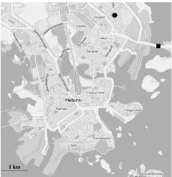
Fig. 1. The measuring locations on Helsinki area. The black circle
presents the Vallila site and the black square shows the place of the automatic traffic counts at It¨av¨ayl¨a road.
Cachier, 2001). Kerminen et al. (1997) studied diesel vehicle exhausts and found that BC mass concentration peaked with aerodynamic diameter of 0.1 µm. Due to their size, the av-erage time these particles spend in the atmosphere is around 6 days and can be transported some thousands of kilometres (Khan et al., 2006).
The crucial question is how urban BC concentrations have developed during the last decades. The main sources of BC have changed because of fuel and technology improvements, both in industrial and commercial sectors. In the 20th cen-tury, BC emissions decreased due to the changes in coal us-age and improvements in diesel technology (Novakov et al., 2003). In the United Kingdom, decrease in BC emissions and concentrations has been detected in the last 40 years (No-vakov and Hansen, 2004). The reductions can be explained by the improved technology, which decreases the emission factors (emitted BC per unit mass of fossil fuel) and clean-ing methods. In Europe, the yearly BC emissions decreased from 0.89 to 0.68 Tg between 1990 and 2000 (Kupiainen and Klimont, 2007). This reduction was mainly due to the de-velopment in Eastern Europe, where a significant decrease of BC emissions was observed especially between 1990 and 1995. The changes in BC concentrations were studied in Tokyo in 1994–2004 and a yearly decrease of 0.88 µg m−3 was observed (Minoura et al., 2006). The main reason was reported to be lower emitting vehicles.
In Helsinki, Finland, BC mass concentration measure-ments have been conducted in three campaigns since 1996. Measurements have been made at the same site in Vallila
located next to one of the main roads leading to the down-town of Helsinki. In Vallila, the annual contribution of BC to PM2.5 and PM10 was found to be 14% and 7%,
respec-tively, in 2000–2001 (Viidanoja et al., 2002). The most im-portant source of BC has been identified to be local traf-fic, which contributes 63% to the concentrations on working days (Pakkanen et al., 2000). Other main contributors are long-range transport and other local sources than traffic. The effect of domestic heating is negligible at the measurement site, since in Helsinki the usage of district heating is most common (Pakkanen et al., 2000). Road traffic emissions have been affected by an increase in the number of vehicles dur-ing the past years. On average, traffic rates have increased 12% in Helsinki between 1996 and 2005 (Lilleberg and Hell-man, 2006). It is reasonable to assume that especially the number of diesel vehicles has increased, since the fraction of diesel powered cars, vans, busses and lorries has increased from 20 to 30% in Finland during this time (M¨akel¨a, 20061). At the same time, exhaust emissions from vehicles have de-creased due to developments in the after-treatment and clean-ing methods of car exhausts.
The purpose of this work is to study the temporal varia-tions in BC concentravaria-tions with different timescales between 1996 and 2005, and to analyze reasons to the observed be-haviour. The analysis is done with data from three mea-surement campaigns. In Sect. 2, the meamea-surements and used methods are introduced. The BC concentrations during each campaign and the seasonal variations are studied in Sect. 3.1. More detailed analysis with weekly and diurnal variations for selected periods is presented in Sect. 3.2 and Sect. 3.3 summarizes variations in traffic patterns in 1996–2005. The effect of traffic and meteorological conditions on the BC concentrations is studied via multiple regression analysis in Sect. 3.4. Finally, conclusions are presented in Sect. 4.
2 Measurements and methods
2.1 Measurement site
Helsinki (60◦10′N, 24◦56′E) itself is located on a relatively flat land at the coast of Gulf of Finland. The area of the city is 686 km2with 560 000 inhabitants. Helsinki together with the neighbouring cities (Vantaa, Espoo, Kauniainen) forms the Helsinki metropolitan area with a total area of 1460 km2 and 1 million inhabitants. The measurements took place in Vallila about 2 km northeast of the downtown of Helsinki (Fig. 1). The measuring site represents a typical urban area of Helsinki and it is in a small opening surrounded by 5–7 storey buildings. It is situated 14 m away from the nearest road, H¨ameentie. This is one of the main roads leading to the city centre and its traffic loads are high especially during rush
1M¨akel¨a, K.: Personal communication, Technical Research
hours. The number of buses using diesel fuel is considerable on the road.
The traffic rates are monitored by the Helsinki City Plan-ning Department. The nearest automatic traffic counting point is by the It¨av¨ayl¨a road on the Kulosaari Bridge, about 1.7 km southeast of the BC measuring site (Fig. 1). Traf-fic data is logged once an hour, and during rush hours four times per hour.
2.2 Black carbon measurements and data selection
The BC measurements were made during three campaigns between 1996 and 2005. The first campaign was from November 1996 to June 1997, the second from September 2000 to May 2001 and the third from March 2004 to Oc-tober 2005. Data during these campaigns were incomplete due to, e.g. power cuts and maintenance operations. Thus, comparisons between different years were done for selected periods, when data from all campaigns existed. In the selec-tion, more weight was given to Campaigns 1 and 3, which had 75% data coverage. For Campaign 2, the coverage was 55%. Four comparable periods were found, two in winter and two in spring. All together, 82 whole days from each campaign was chosen (Table 1).
All measurements were carried out with the aethalome-ters (Hansen et al., 1984). It is an optical instrument where aerosol particles are collected on a filter (quartz tape) and the light transmittance through the filter is measured. To avoid the optical saturation, the filter spot changes at a certain light transmittance value. A more detailed description about the measurement technique is presented in Hansen et al. (1984). Sample air was taken using an inlet about 3.5 m above ground level and fed into the aethalometer inside a measurement container. Only particles with aerodynamic diameter smaller than 2.5 µm were sampled. The aethalometer model, the measuring time resolution and the flow rate varied between the campaigns. In 1996 and 1997, measurements were made with a one-wavelength (880 nm) aethalometer (Magee Scien-tific Aethalometer, model AE-14) with a 10-min time resolu-tion. The flow rate was 16.7 lpm. Two different aethalome-ters operated during Campaign 2. From September 2000 to mid-January 2001, a model AE-20 with a 20-min time reso-lution was used and from mid-January to May 2001 measure-ments were carried out with a 10-min resolution with a mul-tiwavelength model AE-30 (Magee Scientific Aethalometer). In both cases, the same wavelength 880 nm was used for BC measurements and the flow rates were 5.6 lpm and 5.4 lpm, respectively. In 2004–2005, measurements were made with a one-wavelength (880 nm) aethalometer (Magee Scientific Aethalometer, model AE-16) with a 5-min time resolution and a flow rate of 5.2 lpm. The mass absorption cross section of BC used to convert the aethalometer raw signals to BC mass concentrations was 16.6 m2g−1for each campaign.
2.3 Effect of black carbon loading and the correction method
With an aethalometer, the BC concentrations are calculated from the rate of change of attenuation of the light beam. The aethalometer software assumes that the relationship between the rate of change of attenuation and the BC concentration is linear. However, it has been observed that this relationship is usually nonlinear (e.g. Weingartner et al., 2003; Arnott et al., 2005; Virkkula et al., 2007). This nonlinearity leads to underestimation of BC when the filter gets darker, i.e. when attenuation increases. Virkkula et al. (2007) developed a sim-ple algorithm to correct the data. The corrected BC concen-trations were calculated with equation
BCCORRECTED=(1 + k · ATN)BCNON−CORRECTED. (1)
In the Eq. (1), ATN is the light attenuation defined as
−100 ln(I I0−1), where I0and I are the light intensities
be-fore and after the filter, respectively, and k is a constant calcu-lated from the concentration difference before and after the filter spot change. The algorithm assumes that the concen-tration stays stable during the filter spot change (Virkkula et al., 2007). This is not always true, so median k values were calculated for each campaign and were used to cor-rect the data. For the aethalometer used during Campaign 1,
k was 0.0050±0.0003 (s.e) and during Campaign 3 it was
0.0060±0.0004. The k value was not possible to calculate for aethalometer used at the beginning of the Campaign 2 due to the low measuring resolution (20 min). Same applies for the second aethalometer used during Campaign 2, since k values for multiwavelength aethalometers may be incorrect. Therefore, the same k value, which was valid for Campaign 1 and was also obtained by Virkkula et al. (2007), was used to correct the data during Campaign 2. A sensitivity test of the
k values showed that a difference of 0.001 would cause a 4%
and 3.9% error in BC concentrations for the aethalometers used in 2000 and 2001, respectively.
An example how the loading effect correction is affecting the BC concentrations is shown in Fig. 2 for two days in Jan-uary 2005. The discontinuities in uncorrected data are due to the filter spot changes. At the end of each filter spot, the uncorrected concentrations are much smaller than concen-trations at the beginning of the next filter. This effect is due to the loading effect of the filter. The correction algorithm makes the data more continuous and the decrease due to the loading effect disappears. It is evident that the correction made is usually significant and can be as high as 1 µg m−3.
2.4 Meteorological pre-processing model
The meteorological data used in this study was calculated with the meteorological pre-processing model (MPP-FMI) (Karppinen et al., 1997, 2001), which is based on the en-ergy budget method originally developed by van Ulden and Holtslag (1985). The method evaluates turbulent heat
Table 1. The selected data periods, the number of measurement days and the percentage of data included on each period.
Time period No. of days Campaign 1 Campaign 2 Campaign 3 1996–1997 2000–2001 2004–2005 (%) (%) (%) 1.12–17.12 (P1) 17 88 100 76 26.12–8.1 (P2) 14 86 71 79 6.3–3.4 (P3) 29 79 97 100 13.4–4.5 (P4) 22 100 55 100 00:000 12:00 00:00 12:00 00:00 1 2 3 4 5 Local time BC concentration ( µ g m −3 ) Uncorrected Corrected
Fig. 2. The black carbon (BC) mass concentrations (µg m−3) be-fore (grey line) and after (black line) the loading effect correction in 17–18 January 2005.
and momentum fluxes in the boundary layer from synoptic weather observations. The MPP-FMI estimates the hourly time series for the so-called pre–processed meteorologi-cal variables, which are more representative for the whole Helsinki area than variables from a single point measure-ments made, e.g. at the airport. The pre-processed meteo-rological variables include also important, not directly mea-sured variables such as Monin-Obukhov length and mixing height, which are important for determining the dispersion conditions.
2.5 Multiple regression analysis
A multiple regression analysis is used to get information which variables influence to the BC concentrations most, and how much of the concentration variation can be explained by traffic and how much by the meteorological parameters.
In multiple regression analysis, a relationship between de-pendent variable and several indede-pendent variables is stud-ied. In our case, BC concentration is the dependent variable and the traffic rate and meteorological parameters are the in-dependent variables (X1. . . Xn). The idea is to construct a
model, which follows equation
BCpred=b0+b1X1+b2X2+. . . + bnXn, (2) where b0is the intercept and b1. . . bnare the regression coef-ficients (Hair et al., 2006). Variables to the regression model are chosen by minimizing the difference between the mea-sured BC concentrations and BC concentrations obtained from the model. The normalization of the dependent and in-dependent variables before the multiple regression model en-ables one to get also the so-called beta coefficients, which tell the importance of the corresponding variable to the depen-dent variable in relation to the other independepen-dent variables in the model. We used bootstrapping to obtain error estimates for the model parameters and performance indices. In boot-strapping, the used data is divided into 100 subsamples each including arbitrary 5/6 of the original data. The MLR model is constructed for each subset and the final regression coef-ficients, beta coefcoef-ficients, squared R and root mean square error are calculated as arithmetic means and standard devia-tions of each submodel. The bootstrapping gives better esti-mate for model parameters (regression and beta coefficients), eliminates the error caused by outliers and offers more gen-eralized model as an output.
MLR model has an assumption that the variables are nor-mally distributed. However, in our case most of the variables had a lognormal distribution and in order to avoid violating the assumptions of normal distribution, logarithmic transfor-mations were done for BC concentration, traffic rate, wind speed, mixing height and relative humidity. If one wishes to compare beta values of different sampling periods, the dis-tributions have to be similar. This is ensured using Levene’s test (Hair et al., 2006). The data used in MLR calculations had hourly time resolution.
3 Results and discussion
3.1 The annual behaviour of BC concentrations
Monthly boxplots of BC concentrations for each campaign are shown in Fig. 3. Boxplot was drawn if over half of data existed from the corresponding month. The BC concentra-tion peaked in fall and late winter (February) with maxima
0 2 4 a) Campaign 1 0 2 4 BC concentration ( µ g m −3 ) b) Campaign 2
Mar May Jul Sep Nov Jan Mar May Jul Sep 0
2
4 c) Campaign 3
Fig. 3. Monthly boxplots of BC concentrations for each
measure-ment campaign (Campaign 1 from November 1996 to June 1997, Campaign 2 from September 2000 to May 2001 and Campaign 3 from March 2004 to September 2005). Gray lines give the monthly median value and the black boxes define the lower and upper quar-tiles. The straight lines show the interquartile range of each month.
around 1.5 µg m−3. The autumn peaks are likely related to
meteorology, more precisely to mixing layer heights (Pohjola et al., 2000). Late winter is typically the coldest time of year (Drebs, 2002), which may lead to increased BC emissions and strong inversions. The lowest BC concentrations were measured in summer when the median values ranged be-tween 0.8 and 1.3 µg m−3(Fig. 3c). The only exception was in June 1996 when concentration was 1.6 µg m−3(Fig. 3a). The seasonal pattern was especially pronounced during Cam-paign 2 in 2000–2001.
3.2 Median BC concentrations
The BC time series (hourly medians) for the selected periods were plotted in Fig. 4. High concentration episodes can eas-ily be seen and it is evident that those episodes deviate from year to year depending, e.g. on meteorological conditions. The median BC concentrations for the selected periods expe-rienced a slight decrease from 1.11 to 1.00 µg m−3between Campaigns 1 and 3 (Table 2). The concentrations were low-est during Campaign 2 with a median value of 0.93 µg m−3.
The separate examination of each period showed no clear systematic pattern between the campaigns, but the highest concentrations were most often measured during Campaign 1 (periods 1, 2 and 3).
The measured values correspond well with other measured BC concentrations in Helsinki. Pakkanen et al. (2000) used partly the same data as in Campaign 1 and got an aver-age value of 1.38 µg m−3. This value is somewhat higher than our 1.11 µg m−3, even though the used loading effect
Table 2. The median BC concentrations (µg m−3) and quartile de-viations (half of the difference between lower and upper quartiles) measured during each period and campaign.
Period Campaign 1 Campaign 2 Campaign 3 (1996–1997) (2000–2001) (2004–2005) P1 1.43 (0.62) 0.95 (0.35) 1.12 (0.71) P2 1.14 (0.54) 0.97 (0.36) 0.68 (0.46) P3 1.11 (0.61) 0.92 (0.40) 1.04 (0.56) P4 0.86 (0.54) 0.90 (0.51) 1.05 (0.50) All 1.11 (0.60) 0.93 (0.40) 1.00 (0.56)
correction raised BC concentrations in this study. Devi-ations between these two studies rise from the partly dif-ferent time period and from the median value used in this study. Between July 2000 and July 2001 an annual av-erage value of 1.2 µg m−3 was measured by Viidanoja et al. (2002), being again somewhat higher than our result dur-ing Campaign 2. The observed decrease 0.11 µg m−3in ten years in Helsinki is much smaller than the yearly decrease of 0.88 µg m−3 observed in Tokyo, Japan (Minoura et al.,
2006). In Tokyo, traffic rates are much higher and thus the effect of lower traffic emissions is more evident in BC measurements. In Helsinki, the concentration 1.11 µg m−3 in 1996–1997 was already very small compared to Tokyo’s 11 µg m−3in 1996. In general, BC concentrations are lower in Helsinki than in many European cities, where BC concen-trations have been measured. Salma et al. (2004) measured a mean BC concentration of 2.9 µg m−3in Budapest in spring 2002. In London, winter and spring concentrations were measured to be 3.2 and 2.7 µg m−3, respectively, in 1995– 1996 (Kendall et al., 2001). Much higher BC concentrations were measured in Birmingham by Castro et al. (1999) in win-ter 1994 (3.4 µg m−3) and in Vienna by Hitzenberger and
Tohno (2001) in winter 1998–1999 (6.58 µg m−3).
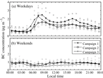
The BC concentrations had a weekly cycle with higher concentrations on weekdays and lower on weekends (Fig. 5). This is apparently related to the lower traffic rates on week-ends. On weekdays, the daily median BC concentrations ranged between 1.3–1.5 µg m−3 during Campaign 1, be-tween 0.9–1.1 µg m−3during Campaign 2 and between 1.1– 1.3 µg m−3 during Campaign 3. Thus, the weekday con-centrations were lowest during Campaign 2, and decreased from Campaign 1 to 3 following the overall medians (Ta-ble 2). On weekends, the concentrations ranged between 0.6–1.1 µg m−3with slightly lower values on Sundays. Be-tween 1996 and 2005, the weekend concentrations systemat-ically decreased.
The diurnal variation of BC concentrations was exam-ined separately for weekdays and weekends (Fig. 6). The effect of traffic was evident on weekdays when the maxi-mum concentration was measured during morning rush hours
1/120 5/12 9/12 13/12 17/12 3 6 9 12 15 18 Campaign 1 Campaign 2 Campaign 3 26/120 30/12 3/01 7/01 3 6 9 12 15 18 6/03 11/03 16/03 21/03 26/03 31/030 3 6 9 12 15 18 BC concentration ( µ g m −3 ) 13/040 18/04 23/04 28/04 3/05 3 6 9 12 15 18 Day
Fig. 4. BC time series during chosen periods. Black solid line stands for Campaign 1, light-gray solid line for Campaign 2 and dark-gray
dash-dotted line for Campaign 3. Values are hourly medians calculated from the raw data.
Mon Tue Wed Thu Fri Sat Sun
0 0.5 1 1.5 BC concentration ( µ g m −3 ) Campaign 1 Campaign 2 Campaign 3
Fig. 5. Median black carbon concentrations on different weekdays
during Campaigns 1 (stars), 2 (circles) and 3 (crosses).
between 05:00 and 09:00 a.m. (Fig. 7a). The peaks related to morning rush hours were the same 2.4 µg m−3during
Cam-paigns 1 and 3, and lower (1.7 µg m−3) during Campaign 2.
The afternoon maximum, related to afternoon rush hours, was most evident during Campaign 1 reaching a value of 2 µg m−3. The afternoon peaks were systematically lower than the morning peaks due to the stronger turbulent mix-ing and increased mixmix-ing layer heights. In daytime, when also the traffic rates are high, the BC concentrations were evidently elevated during Campaign 1, suggesting greater effect of traffic. The daytime concentrations were lowest during Campaign 2 following the pattern of total concen-trations. The nocturnal concentrations were similar, around 0.5 µg m−3, during the campaigns.
On weekends, the diurnal pattern differed considerably from that on weekdays (Fig. 6b). Minimum values were mea-sured in the early morning and maximum values at night and
0 1 2 3 4 (a) Weekdays 00:000 03:00 06:00 09:00 12:00 15:00 18:00 21:00 00:00 1 2 3 Local time BC concentration ( µ g m −3 ) (b) Weekends Campaign 1 Campaign 2 Campaign 3
Fig. 6. Diurnal variations in BC concentrations (black lines) on (a) weekdays and (b) weekends for each measurement campaign.
Stars are the BC concentrations during Campaign 1, circles are the BC concentrations during Campaign 2 and crosses represent the BC concentrations during Campaign 3. Values were calculated as me-dians from the hourly data and error estimates (gray marks) are the lower and upper quartiles.
afternoon. Friday and Saturday are the most typical days for people to go out in Helsinki, and the raised nocturnal concen-trations are caused by the numerous taxis and buses, which are typically diesel powered (see also Fig. 7b). In addition to the intense diesel-powered traffic, low mixing heights raise the nocturnal concentrations. The diurnal variation of BC was similar to the diurnal behaviour of accumulation mode particle concentrations measured in Helsinki (Laakso et al.,
2003; Hussein et al., 2004). This was the case especially dur-ing weekends, when diurnal variations were rather small and maximum was measured at night.
3.3 Traffic trends
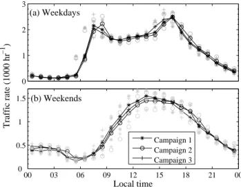
The major source of BC is the local traffic, which in our case refers mainly to the vehicles on the road (H¨ameentie) next to the measurement site. To estimate the effect of traffic on the measured concentrations, it is important to know the traffic intensities on H¨ameentie. Online traffic monitoring was only made at It¨av¨ayl¨a, so the traffic rates on H¨ameentie needed to be derived from these. The traffic rates have been counted in campaigns on H¨ameentie, and the comparison of these campaign traffic rates with the traffic rates on It¨av¨ayl¨a, en-abled us to calculate transformation coefficients between the two roads. The coefficients were determinated by fitting a straight line to the data measured at these two locations. To get the traffic rates on H¨ameentie, the traffic rates on It¨av¨ayl¨a needed to be multiplied by values 0.576 (R2=0.998), 0.553 (R2=0.995) and 0.564 (R2=0.997) for Campaigns 1, 2 and 3, respectively. This shows that the traffic rates on these two roads are correlating well, but are about 50% less on H¨ameentie than on It¨av¨ayl¨a.
Overall, the daily traffic rates have increased from 29 700 to 30 000 vehicles day−1 on H¨ameentie between Cam-paigns 1 and 3. This increase occurred mainly on week-days, while on weekends, the traffic rates were similar (19 750 vehicles day−1) during Campaigns 1 and 3. The
traf-fic rates were lowest (29 600 vehicles day−1) during
Cam-paign 2, agreeing with the lowest BC concentrations. How-ever, changes in traffic rates were marginal and this correla-tion should be considered cautiously.
On weekdays (Fig. 7a), the traffic rates followed a typ-ical rush hour related pattern with maxima in the morning (05:00–10:00 a.m.) and afternoon (03:00–06:00 p.m.). The traffic pattern on weekends (Fig. 7b) showed highest traffic rates in daytime during all campaigns with slightly higher traffic intensities during Campaign 1. The weekend night– time traffic rates seemed to have decreased from 1996 to 2005. The differences in the diurnal variation of traffic rates between the campaigns were small compared to the diurnal behaviour of BC concentrations (Fig. 6) implying that the number of vehicles is not the only factor affecting the centrations. On weekends, the diurnal behaviour of BC con-centrations was not as evidently related to the diurnal varia-tions of traffic rates as on weekdays.
As already was mentioned, the traffic rates itself did not explain all the variation in the BC concentrations. The mea-sured BC concentrations are also affected by other local and distant sources. The effect of meteorology on the measured concentrations is studied in Sect. 3.3. Some of the differ-ences between the behaviour of BC concentrations and the behaviour of traffic can be explained by the uncertainties in traffic counts, which do not take into consideration whether
0 1 2 3 (a) Weekdays 00 03 06 09 12 15 18 21 00 0 0.5 1 1.5 Local time Traffic rate (1000 hr −1 ) (b) Weekends Campaign 1 Campaign 2 Campaign 3
Fig. 7. Diurnal variations in traffic rates (black lines) on (a)
week-days and (b) weekends for each measurement campaign. Stars are the traffic rates during Campaign 1, circles are the traffic rates dur-ing Campaign 2 and crosses are the traffic rates durdur-ing Campaign 3. Values were calculated as medians from the hourly data and error estimates (gray marks) are the lower and upper quartiles.
vehicles are diesel or gasoline powered, and differences in vehicle emissions. The effect of cleaner exhaust emissions from diesel powered vehicles on the BC concentration was examined by comparing the nocturnal vehicle number-scaled BC concentrations on weekends, when vehicles are mainly expected to be diesel-powered taxis and buses. The taxi pool is always fairly new in Helsinki and the effect of improved technology is easier to detect during intensive taxi traffic. Typically, the average age of the car pool is high in Fin-land. Passenger cars mean age was 10.4 years in Finland in 2003, while in UK and France corresponding ages were 6.8 and 8.0 years (http://www.autoalantieto.fi/vanhauusi.asp), respectively. The hourly BC concentrations were scaled with hourly traffic rates between 02:00 and 04:00 a.m. We found that the vehicle number-scaled BC mass con-centrations were 0.0028±0.0005 (s.e), 0.0022±0.0005 and 0.0020±0.0002 µg m−3 for Campaigns 1, 2 and 3,
respec-tively. Thus, roughly the effect of diesel vehicle emissions on the BC concentrations seems to have decreased, follow-ing the engine development and better exhaust after treat-ment. These estimates have a large uncertainty and should be considered with caution, since nocturnal traffic includes also some gasoline cars and BC concentrations include con-tribution of other local sources and long-range transport. 3.4 Multiple regression analysis
Besides traffic, meteorology has a strong effect on BC con-centrations. The local meteorology affects the dispersion of pollutants and long-range transport has been identified to be one of the main factors affecting BC concentrations, with an
Table 3. Results from the multiple regression analysis for all data, weekdays and weekends separately, and for Campaigns 1, 2 and 3
(p<0.05). Optimized models were obtained with three variables: traffic (Tr), wind speed (U ) and mixing height (Hm). The model parameters squared R, root mean square error (rmse), intercept (int), and regression coefficients b and beta coefficients β of independent variables are also listed. R2 rmse±std int b β std (β) All 54 0.22±0.00 0.91±0.01 Tr 0.50 0.63 0.01 U −0.73 −0.48 0.01 Hm −0.17 −0.17 0.01 Weekdays 59 0.21±0.00 0.83±0.01 Tr 0.50 0.69 0.01 U −0.70 −0.46 0.01 Hm −0.12 −0.12 0.01 Weekends 48 0.20±0.00 0.97±0.02 Tr 0.36 0.39 0.01 U −0.81 −0.60 0.01 Hm −0.22 −0.28 0.01 Campaign 1 58 0.21±0.00 1.06±0.02 Tr 0.54 0.69 0.01 U −0.71 −0.47 0.01 Hm −0.21 −0.22 0.01 Campaign 2 53 0.18±0.00 0.68±0.02 Tr 0.42 0.65 0.01 U −0.56 −0.37 0.01 Hm −0.13 −0.14 0.01 Campaign 3 60 0.23±0.00 1.07±0.03 Tr 0.55 0.62 0.01 U −0.90 −0.57 0.01 Hm −0.21 −0.22 0.01 P1 P2 P3 P4 0 0.5 1 1.5 2 Traffic rate (1000 hr −1 ) (a) P1 P2 P3 P4 0 2 4 6 U (m s −1 ) (b) P1 P2 P3 P4 −10 −5 0 5 10 T ( ° C) (c) P1 P2 P3 P4 960 980 1000 1020 p (hPa) (d) P1 P2 P3 P4 40 60 80 100 RH(%) (e) P1 P2 P3 P4 0 500 1000 H m (m) (f) Campaign 1 Campaign 2 Campaign 3
Fig. 8. Median (a) traffic rate (1000 vehicles h−1), (b) wind speed
U (m s−1), (c) temperature T (◦C) (d) pressure p (hPa), (e) relative
humidity RH (%) and mixing height Hm (m) for all four periods during Campaigns 1, 2 and 3.
average value of 0.4 µg m−3(Pakkanen et al., 2000). A mul-tiple regression analysis was made to identify the relation-ships between BC concentrations, traffic and meteorological variables.
Multiple regression models were constructed for differ-ent situations, including whole data, winter and spring
sepa-rately, weekdays and weekends sepasepa-rately, and for each cam-paign. The optimized models were in most cases obtained with three independent variables. Traffic and wind speed were always present in the models and the third variable var-ied between mixing height, pressure, temperature and rela-tive humidity. The median values of these model variables during the selected periods are shown in Fig. 8. Changing the third variable did not have a great effect on the model and in the final models the same three variables were used to get the different cases more comparable. Traffic and wind speed were automatically included to the multiple regression models and the third one was chosen to be the mixing height. These three variables gave most often the best results.
The multiple regression analysis for all data (R2=54%) confirmed traffic having the most important effect on BC concentrations with a beta coefficient of 0.63 (Table 3). Of the meteorological variables, wind speed had the highest in-fluence on the BC concentrations with a beta coefficient of
−0.48. The negative sign means inverse relationship be-tween the wind speed and BC concentrations: the lower the wind speed, the higher the concentration due to the mixing of pollutants. Beta coefficient for mixing height was also neg-ative (−0.17). High mixing height allows the air pollution mix into a larger air volume and lower concentrations at the surface are measured. Division into weekdays and weekends showed traffic having the greatest effect on BC concentra-tions on weekdays but not on weekends, when the wind speed had the strongest influence (Table 3). The latter, was al-ready suggested by the diurnal patterns of BC concentration
and traffic rate, which seemed to have lower connection on weekends (Figs. 6 and 7). The multiple regression model was poorer on weekend than on weekdays. Adding more variables did not improve the model on weekends, suggest-ing that there was some misssuggest-ing variable or variables, which were not included to the available variables such as the long-range transport. For example, we did not have the informa-tion about the changes in the emission sources around Eu-rope during the studied period. Thus, the changes caused by the distant sources remained unknown. On the other hand, also the number of weekend samples was much lower than the number of weekday samples, which increases the uncer-tainty.
A multiple regression analysis was also made separately for winter and spring periods (Not shown). The opti-mized model was better for winter (R2=62%) than for spring (R2=52%) and differences were small between the seasons. The effect of traffic was slightly larger during winter than spring (beta coefficients of 0.66 and 0.62, respectively), while the influence of wind speed was the same. The mix-ing height was more important factor durmix-ing sprmix-ing than in winter.
To compare whether the contribution of traffic on the mea-sured BC concentrations had changed during the ten years, multiple regression models were made separately for each campaign (Table 3). The Levene’s test showed that with 95% confidence the variances of traffic were the same between the campaigns, meaning comparable beta coefficients between the campaigns. The squared R’s were between 53 and 60% during the campaigns. In all cases, traffic had the highest in-fluence on the BC concentrations before the wind speed. The effect of wind speed and mixing height did not have any sys-tematic trend between the campaigns and for both, the lowest effects were observed during Campaign 2. The effect of traf-fic, on the other hand, had a decreasing trend between the beta coefficients from 0.69 to 0.62 indicating a decreased in-fluence of traffic on the BC concentrations. The number of vehicles had increased in Helsinki and thus, the decreasing effect needs to be related to the cleaner exhaust emissions. This supports the rough estimate for the diesel vehicle emis-sions obtained in Sect. 3.3.
The decrease in BC concentrations between Campaigns 1 and 3 could be explained by the decreased exhaust emissions from the (diesel) vehicles. The decrease in concentrations occurred especially during rush hours, when the traffic rates were highest and the decreased exhaust emissions most vis-ible. The traffic rate was the most important variable affect-ing the BC concentrations duraffect-ing Campaign 2, so the BC concentration minimum was at least partly explained by the lower traffic rates, even though the deviations between the campaigns were small.
4 Conclusions
The purpose of this study was to investigate the temporal variation in BC concentrations in Helsinki between 1996 and 2005. Measurements were made in three campaigns in Vallila, which is located two kilometres of the centre of Helsinki. One of the main roads leading to the city cen-tre is located 10 m away from the measurements site. The first campaign took place from November 1996 to June 1997, the second from September 2000 to May 2001 and the third from March 2004 to October 2005. Detailed analysis, with weekly and diurnal cycles and multiple regression analysis, was made for a selected periods when data from each cam-paign existed. All together four periods and a total number of 82 days from each campaign was chosen. Two periods were in winter and two in spring, respectively.
The BC concentrations showed annual pattern with max-ima in late winter and fall. In late winter, enhanced emissions and low mixing raise the concentrations, while in fall the el-evations can be explained by meteorological conditions. The comparison of the different campaign showed a slight de-crease in BC concentrations from 1.11 to 1.00 µg m−3
be-tween 1996 and 2005. The decrease occurred especially on daytime during the weekdays, when traffic intensities were highest. Systematically, lower concentrations were measured during Campaign 2 following the slightly lower traffic rates. The only exception was the weekend concentrations when the concentrations decreased between the campaigns.
The optimized multiple regression models to predict the BC concentrations were obtained with three variables: traf-fic, wind speed and mixing height. On weekdays, traffic had clearly the highest influence before the wind speed, and on weekends, the effect was the other way around. On week-ends, the traffic rates were much lower causing the meteoro-logical factors becoming more important. Of the three vari-ables, the mixing height was always the least explanatory one. The separate examination of each campaign showed a decreased influence of traffic on the BC concentrations. The beta coefficients decreased from 0.69 to 0.62. Since the traffic rates have increased between Campaign 1 and 3, the decreasing effect is very likely caused by cleaner exhaust emissions due to engine and fuel development, and exhaust after treatment. At our sampling site, the vehicle number-scaled BC concentrations have decreased from 0.0028 to 0.0020 µg m−3between Campaigns 1 and 3. This indicates a decreased effect of vehicle exhausts on the BC concentra-tions. It is worth of mentioning, that these values are very rough and may be different for different sites. The decreased BC exhaust emissions most probably caused the decrease in the BC concentrations during 1996–2005, while the lowest concentrations during Campaign 2 were at least partly ex-plained by the lower traffic rates.
Acknowledgements. For financial support we would like to thank Research Foundation of the University of Helsinki, Maj and Tor
Nessling Foundation, National Technology Agency (TEKES, Grant # 40462/03) and the Ministry of Environment. T. Koistinen and H. Sepp¨al¨a from City Planning Department and M. Dal Maso and L. Sogacheva from University of Helsinki are acknowledged for their help in this study.
Edited by: K. Lehtinen
References
Arnott, W. P., Hamasha, K., Moosm¨uller, H., Sheridan, P. J., and Ogren, J. A.: Towards aerosol light absorption measurements with a 7-wavelength Aethalometer: Evaluation with a photoa-coustic instrument and 3 wavelength nephelometer, Aerosol Sci. Technol., 39, 17–29, 2005.
Castro, L. M., Pio, C. A., Harrison, R. M., and Smith, D. J. T.: Carbonaceous aerosol in urban and rural European atmospheres: estimation of secondary organic carbon concentrations, Atmos. Environ., 33, 2771–2781, 1999.
Drebs, A., Nordlund, A., Karlsson, P., Helminen, J., and Rissanen, P.: Climatological statistics of Finland 1971–2000 (in Finnish), Finnish Meteorological Institute, Helsinki, 24 pp., 2002. Hair, J. F., Black, W. C., Babin, B. J., Anderson, R. E., and Tatham,
R. L.: Multivariate data analysis (Sixth edition), Pearson Educa-tion, New Jersey, Chapter 4, 2006.
Hansen, A. D. A., Rosen, H., and Novakov, T.: The aethalometer: an instrument for real-time measurement of optical absorption by aerosol particles, Sci. Tot. Environ., 36, 191–196, 1984. Hitzenberger, R. and Tohno, S.: Comparison of black carbon (BC)
aerosols in two urban areas – concentrations and size distribu-tions, Atmos. Environ., 35, 2153–2167, 2001.
Hussein, T., Puustinen, A., Aalto, P., M¨akel¨a, J., H¨ameri, K., and Kulmala, M.: Urban aerosol number size distributions, Atmos. Chem. Phys., 4, 391–411, 2004,
http://www.atmos-chem-phys.net/4/391/2004/.
Jacobson, M. Z.: Strong radiative heating due to the mixing state of black carbon in atmospheric aerosols, Nature, 409, 695–697, 2001.
Jiang, M., Marr, L., Dunlea, E., Herndon, S., Jayne, J., Kolb, C., Knighton, W., Rogers, T., Zavala, M., Molina, L., and Molina, M.: Vehicle fleet emissions of black carbon, polycyclic aromatic hydrocarbons, and other pollutants measured by a mobile labora-tory in Mexico City, Atmos. Chem. Phys., 5, 3377–3387, 2005, http://www.atmos-chem-phys.net/5/3377/2005/.
Karppinen, A., Joffre, S. M., and Vaajama, P.: Boundary-layer pa-rameterization for Finnish regulatory dispersion models, Int. J. Environ. Pollut., 8, 557–564, 1997.
Karppinen, A., Joffre, S. M., and Kukkonen J.: The refinement of a meteorological preprocessor for the urban environment, Int. J. Environ. Pollut., 14, 1–9, 2001.
Keeler, G., Morishita, M., and Young, L.-H.: Characterization of complex mixtures in urban atmospheres for inhalation exposure studies, Experimental and Toxicologic Pathology, 57, 19–29, 2005.
Kendall, M., Hamilton, R. S., Watt, J., and Williams, I. D.: Char-acterisation of selected speciated organic compounds associated with particulate matter in London, Atmos. Environ., 35, 2483– 2495, 2001.
Kerminen, V.-M., M¨akel¨a, T., Ojanen, C., Hillamo, R., Vilhunen, J., Rantanen, L., Havers, N., von Bohlen, A., and Klockow, D.: Characterization of the particulate phase in the exhaust from a diesel car, Environ. Sci. Technol., 31, 1883–1889, 1997. Khan, A. J., Li, J., and Husain, L.: Atmospheric
trans-port of elemental carbon, J. Geophys. Res., 111, D04303, doi:10.1029/2005JD006505, 2006.
Kupiainen, K. and Klimont, Z.: Primary emissions of fine car-bonaceous particles in Europe, Atmos. Environ., 41, 2156–2170, 2007.
Laakso, L., Hussein, T., Aarnio, P., Komppula, M., Hiltunen, V., Viisanen, Y., and Kulmala, M.: Diurnal and annual characteris-tics of particle mass and number concentrations in urban, rural and Arctic environments in Finland, Atmos. Environ., 37, 2629– 2641, 2003.
Lilleberg, I. and Hellman, T.: Traffic development in Helsinki 2005, Helsinki City Planning Department, p. 5, 2006 (in Finnish). Minoura, H., Takahashi, K., Chow, J. C., and Watson, J. G.:
Multi-year trend in fine and coarse particle mass, carbon, and ions in downtown Tokyo, Japan, Atmos. Environ., 40, 2478–2487, 2006. Novakov, T., Ramanathan, V., Hansen, J. E., Kirchstetter, T. W., Sato, M., Sinton, J. E., and Sathaye, J. A.: Large historical changes of fossil-fuel black carbon aerosols, J. Geophys. Res. Lett., 30, 1324, doi:10.1029/2002GL016345, 2003.
Novakov, T. and Hansen, J. E.: Black carbon emissions in the United Kingdom during the past four decades: an empirical anal-ysis, Atmos. Environ., 38, 4155–4163, 2004.
Pakkanen, T., Kerminen, V.-M., Ojanen, C., Hillamo, R., Aarnio, P., and Koskentalo, T.: Atmospheric black carbon in Helsinki, Atmos. Environ., 34, 1497–1506, 2000.
Pohjola, M., Kousa, A., Aarnio, P., Koskentalo, T., Kukkonen, J., H¨ark¨onen, J., and Karppinen, A.: Meteorological interpretation of measured urban PM2.5 and PM10 concentrations in Helsinki metropolitan area, Air pollution VIII, Wessex Institute Press, Southampton, UK, 689–698, 2000.
Pope, C. A., Burnett, R., Thun, M., Calle, E., Krewski, D., Ito, K., and Thurston, G.: Lung cancer, cardiopulmonary mortality, and long term exposure to fine particulate air pollution, J. American Medical Association, 287, 1132–1140, 2002.
Ruellan, S. and Cachier, H.: Characterisation of fresh particulate vehicular exhausts near a Paris high flow road, Atmos. Environ., 35, 453–468, 2001.
Salma, I., Chi, X., and Maenhaut, W.: Elemental and organic car-bon in urban canyon and background environments in Budapest, Hungary, Atmos. Environ., 38, 27–36, 2004.
Stoeger, T., Reinhard, C., Takenaka, S., Schroeppel, A., Karg, E., Ritter, B., Heyder, J., and Schulz, H.: Instillation of six different ultrafine carbon particles indicates a surface area threshold dose for acute lung inflammation in mice, Environ. Health Perspect., 114, 328–333, 2006.
Szidat, S., Jenk, T. M., Synal, H.-A., Kalberer, M., Wacker, L., Ha-jdas, I., Kasper-Giebl, A., and Baltensperger, U.: Contributions of fossil fuel, biomass-burning, and biogenic emissions to car-bonaceous aerosols in Zurich as traced by14C, J. Geophys. Res., 111, D07206, doi:10.1029/2005JD006590, 2006.
van Ulden, A. and Holtslag, A.: Estimation of boundary layer pa-rameters for diffusion applications, J. Appl. Meteor., 24, 1196– 1207, 1985.
R., Aarnio, P., and Koskentalo, T.: Organic and black carbon in PM2.5and PM10: 1 year of data from an urban site in Helsinki,
Finland, Atmos. Environ., 36, 3183–3193, 2002.
Virkkula, A., M¨akel¨a, T., Yli-Tuomi, T., Hirsikko A., Koponen, I. K., H¨ameri, K., and Hillamo, R.: A simple procedure for correct-ing loadcorrect-ing effects of aethalometer data, J. Air Waste Manage. Assoc., 57, 1214–1222, 2007.
Watson, J. G., Chow, J., Lowenthal, D., Pritchett, L., and Fra-zier, C.: Differences in the carbon composition of source profiles for diesel- and gasoline-powered vehicles, Atmos. Environ., 28, 2493–2505, 1994.
Weingartner, E., Saathoff, H., Schnaiter, M., Streit, N., Bitnar, B., and Baltensperger, U.: Absorption of light by soot particles: de-termination of the absorption coefficient by means of aethalome-ters, J. Aerosol Sci., 34, 1445–1463, 2003.