HAL Id: tel-01599049
https://tel.archives-ouvertes.fr/tel-01599049
Submitted on 1 Oct 2017HAL is a multi-disciplinary open access archive for the deposit and dissemination of sci-entific research documents, whether they are pub-lished or not. The documents may come from teaching and research institutions in France or abroad, or from public or private research centers.
L’archive ouverte pluridisciplinaire HAL, est destinée au dépôt et à la diffusion de documents scientifiques de niveau recherche, publiés ou non, émanant des établissements d’enseignement et de recherche français ou étrangers, des laboratoires publics ou privés.
transition du Pléistocène moyen (MIS 31 et MIS 11)
dans la péninsule Ibérique
Dulce Oliveira
To cite this version:
Dulce Oliveira. Comprendre les périodes chaudes pendant et après la transition du Pléistocène moyen (MIS 31 et MIS 11) dans la péninsule Ibérique. Sciences de la Terre. Université de Bordeaux, 2017. Français. �NNT : 2017BORD0598�. �tel-01599049�
THÈSE PRÉSENTÉE POUR OBTENIR LE GRADE DE
DOCTEUR DE
L’UNIVERSITÉ DE BORDEAUX
ÉCOLE DOCTORALE: SCIENCES ET ENVIRONNEMENTS SPÉCIALITÉ: SEDIMENTOLOGIE MARINE ET PALEOCLIMATS
Par Dulce OLIVEIRA
COMPRENDRE LES PERIODES CHAUDES PENDANT ET
APRES LA TRANSITION DU PLEISTOCENE MOYEN
(MIS 31 ET MIS 11) DANS LA PENINSULE IBERIQUE
Sous la direction de: María Fernanda SANCHEZ GOÑI
Soutenue le 23 Mai 2017
Membres du jury:
M. MCMANUS Jerry, Professeur, University of Columbia Rapporteur
M. FLETCHER William, Senior Lecturer, University of Manchester Rapporteur Mme ABRANTES Fátima, Directrice de Recherche, Instituto Português do Mar e da Atmosfera Examinatrice Mme DESPRAT Stéphanie, Maître de Conférences, EPHE PSL Research University,
Université de Bordeaux Examinatrice
Mme NAUGHTON Filipa, Chargé de Recherche, Instituto Português do Mar e da Atmosfera Co-encadrante M. TRIGO Ricardo, Professeur/Directeur de Recherche, Instituto Dom Luiz-IDL,
Universidade de Lisboa
Co-encadrant et Président du Jury Mme SANCHEZ GOÑI María Fernanda, Professeur/Directrice d'Etudes,
Résumé: L'étude des interglaciaires passés qui sont des périodes chaudes avec un volume de glace réduit comme l’interglaciaire actuel, l'Holocène, est cruciale pour comprendre le climat futur. Ce travail apporte de nouvelles informations sur le climat des interglaciaires clés, les stades isotopiques marins (MIS) 11 et 31, considérés comme des analogues au réchauffement global projeté. Une analyse pollinique des sédiments du Site IODP U1385 (marge sud-ouest ibérique) a été effectuée à haute résolution, ce qui permet de comparer directement les variations de la végétation (atmosphère) avec celles de la température des eaux de surface océaniques. Nos données montrent qu’à l’échelle orbitale, la forêt du sud-ouest de l’Europe pendant le MIS 11 est principalement influencée par la précession alors que pendant le MIS 31, malgré des valeurs de précession extrêmes, le forçage dominant est l’obliquité, favorisant une végétation moins méditerranéenne et un régime climatique tempéré. De plus, la variabilité millénaire apparaît comme une caractéristique persistante mais les épisodes de refroidissement varient en intensité et durée en fonction des conditions limites qui favorisent un forçage prédominant des hautes ou basses latitudes. Enfin, nous examinons l'expression régionale de l'Holocène et de ses analogues orbitaux, les MIS 11c et 19c dans le sud-ouest de l’Europe. Ceci révèle que l'optimum Holocène se distingue par un plus fort développement forestier et donc que les MIS 11c et 19c ne sont pas des analogues à l’Holocène pour notre zone d’étude. Grâce à une comparaison modèle-données, nous montrons aussi que la forêt interglaciaire dans cette région est principalement contrôlée par la précession en influençant les précipitations hivernales, facteur critique pour le développement de la forêt méditerranéenne, tandis que le CO2 joue un rôle
négligeable.
Mots clés: Climat interglaciaire, MIS 11, MIS 31, Analogues potentiels de l’Holocène,
Végétation méditerranéenne, Analyse pollinique des archives marines.
Title: Understanding warm periods within and after the Mid Pleistocene Transition (MIS 31 and 11) in the Iberian Peninsula
Abstract: The study of past interglacials, periods of reduced ice volume like our present
interglacial, the Holocene, is crucial for understanding the future climate. This work provides new insights into the intensity and climate variability of key interglacials, namely Marine Isotopic Stages (MIS) 11 and 31, considered as analogues for the projected global warming. A high resolution pollen analysis at IODP Site U1385 off SW Iberia was performed, which enables a direct comparison between atmospheric-driven vegetation changes and sea surface temperature variability. At orbital timescale, this thesis shows that the dominant orbital forcing on the SW European forest was different between the interglacials of the 100-ky (MIS 11) and 41-ky (MIS 31) worlds. While during MIS 11 its weak precessional forcing predominates, during MIS 31 its extreme precession forcing is dwarfed by the prevailing influence of obliquity leading to a temperate climate regime as shown by a less Mediterranean character of the vegetation. This work also shows that millennial-scale variability was a pervasive feature and suggests that the different intensity and duration of the cooling events in SW Iberia was related to different atmospheric and oceanic configurations modulated by high or low-latitude forcing depending on the baseline climate states. Finally, this study examines the dominant forcing underlying the regional expression of the Holocene and its orbital analogues, MIS 11c and 19c, over SW Iberia using a data-model comparison approach. This comparison reveals that the Holocene optimum stands out for its higher forest development and therefore these interglacials cannot be considered as analogues for the Holocene vegetation and climate changes in Iberia. Additionally, it shows that the SW Iberian forest dynamics during these interglacials were primarily controlled by precession through its influence on winter precipitation, which is critical for the Mediterranean forest development whereas CO2 played a negligible role.
Keywords: Interglacial climate, MIS 11, MIS 31, Potential Holocene analogues, Mediterranean
Para ti Gabriel
For a billion years the patient Earth amassed documents and inscribed them with signs and pictures which lay unnoticed and unused. Today, at last, they are waking up, because man has come to rouse them. Stones have begun to speak, because an ear is there to hear them. Layers become history and, released from the enchanted sleep of eternity, life's motley, never-ending dance rises out of the black depths of the past into the light of the present.
This dissertation would not have been possible without the support of many people and institutions. It is a pleasure to express my sincere gratitude to all who contributed to this work and made my dream of doing this doctoral research come true…
Tudo começou com um sonho no final da licenciatura… e depois de percorrida uma longa e atribulada viagem chego a esta fase final de “weee, terminei o doutoramento!!!” Ciente de que as melhores viagens só se fazem em boa companhia, quero expressar a minha gratidão às várias pessoas e instituições que, de diferentes formas, contribuíram para a concretização deste sonho…
First, I would like to thank my exceptional team of French supervisors, Prof. Dr. Maria F. Sánchez Goñi and Dr. Stéphanie Desprat, and Portuguese co-supervisors, Dr. Filipa Naughton and Prof. Dr. Ricardo Trigo. Each of you was very important on its own way and this PhD project would not have been possible without your guidance, encouragement and friendship. Thank you all for your help through constructive comments and reviews on the numerous abstracts, presentations and manuscripts. I sincerely hope that this PhD research has been only the beginning of a series of successful collaborations.
- Merci Maria for giving me the opportunity to do my PhD in the University of Bordeaux and with the excellent “paleo” team. Merci Stéphanie for accepting me as a PhD student, even if it was not official. Maria and Stéphanie, throughout these years your enthusiasm for debating anything related to paleoclimate and your love for palynology has been truly contagious. It has been a great pleasure working with you. This PhD research would not have become a reality without your vision, teaching and much appreciated scientific and personal support. - À Filipa e ao Dr. Ricardo Trigo, agradeço por todo o apoio e confiança depositada em mim desde o mestrado em 2011 na FCUL. As palavras serão sempre poucas para vos agradecer pela experiência e sabedoria partilhados que sempre me deixaram (e deixam!) vontade de fazer mais e melhor! Filipa, és sem dúvida uma investigadora de alma e coração e serás sempre a minha Amiga coach… obrigado por tudo mas principalmente por me “apresentares” os pollens e a paleo! Ao Dr. Ricardo Trigo não posso deixar de agradecer as suas observações construtivas que sempre me incentivaram a “ir mais longe” e me tanto me ajudaram na reconstrução dos padrões de circulação atmosférica.
I am deeply grateful to all members of the jury for agreeing to revise my PhD thesis and for their positive and helpful feedback and discussions in the defense. Moreover, I would like to acknowledge to all the people who worked with me on the different manuscripts of this PhD research.
Special thanks to the scientists and technicians of the Integrated Ocean Drilling Program (IODP) Expedition 339: The Mediterranean outflow, the crew of the JOIDES Resolution and the Bremen Core Repository staff without whom studying Site U1385 would not have been possible.
CLI/100157/2008) and CCMAR (FCT Research Unit - UID/Multi/04326/2013) are gratefully acknowledged. Additional funding for participation in the 11th Urbino Summer School in Paleoclimatology in Italy and in several international scientific meetings was provided by the LEFE-INSU IMAGO WarmClim project, PAGES (Past Global Changes), AFEQ-CNF INQUA (Association Française pour l'Etude du Quaternaire - CNF INQUA), INQUA (International Union for Quaternary Research), APLF (Association des Palynologues de Langue Française) and ECORD (European Consortium for Ocean Research Drilling). Funds provided by the project PHC STAR MEDKO allowed my training on different lipid biomarkers from the Mediterranean cores at the University of Hanyang, South Korea.
I am indebted to my main host institutions, the University of Bordeaux and Instituto Português do Mar e da Atmosfera (IPMA, former LNEG) for providing me the opportunity to perform my PhD research in a great human and scientific environment.
- Un grand merci à toutes les membres de l’équipe paleo, l’équipe technique du laboratoire EPOC and PhD students from the Unv. of Bordeaux that somehow supported me and made my time in Bordeaux a very enjoyable one, namely: Johan, Anne-Laure, Josue, Cesar, Frédérique, Philippe, Giovanni, Ludovic, Marie-Hélène, Vicent, Melanie, Léo, Léa, Mathylde, Salomé, Coralie, Bárbara, Amna, Clement, Calypso, Anna and Melina.
- Special thanks go out to all the members of the “PhD survivors” group for their friendship, help and support. MERCI for all the nice moments during the every day lunches, breaks and several nights. My stay in Bordeaux would not have been such a great experience without you – my best french friends – Léo, Melanie, Léa, Salomé and Childeric.
- Um muito obrigado com carinho a todo o pessoal da Divisão de Geologia e Georecursos Marinhos do IPMA pela partilha de experiências, dúvidas, questões e saberes desde o mestrado no LNEG, e que, de alguma forma, me ajudaram a chegar ao final desta etapa do meu percurso académico. Um agradecimento especial à Dra. Fátima Abrantes, a “mentora” do nosso departamento, e a todos os que demonstraram interesse e apoiaram o meu trabalho: Teresa, Antje, Emilia, Cristina Lopes, Isabelle, Susana, Montse, Zuzia, Pedro, Ana Rodrigues, Dona Apolónia, Daniel, Warley e Cremilde.
- Muito obrigada, de coração, ao pessoal “da sala das lupas” - Andreia, Catarina, Ana, Cristina, Lélia, Sandra, Célia e Isabel - pelo constante apoio e incentivo nas diversas fases desta viagem….e por muitas outras razões que não cabem nestas breves palavras. Muito muito obrigado por tudo, sobretudo pela Amizade preciosa.
Não diretamente envolvidos no meu trabalho científico, mas naturalmente imprescindíveis no meu bem-estar, essenciais para conseguir realizar as tarefas propostas, cumprir prazos estabelecidos e terminar o meu doutoramento, quero agradecer sinceramente:
À Andreia, amiga de sempre e para sempre. Obrigada pela ininterrupta e incansável ajuda, a qualquer hora do dia e noite, quer chova ou faça sol. Sem ti, este trabalho não teria sido sequer começado! Obrigada por tudo e mais um “cadito”!!
À Celina, “irmã” construída desde infância e que me faz acreditar que as ligações e afinidades são efetivamente transversais ao tempo e à distância. Obrigada por estares sempre comigo. À minha “família da Amadora", Alexandra, Dona Lúcia e Leandro, que partilhou e viveu comigo as angústias e alegrias deste projeto. Obrigado por todo o genuíno apoio, encorajamento, incentivo e carinho. Muito obrigada por serem tão especiais!
acolhido na vossa casa, me terem recebido tão bem e por toda a Amizade!
Um sincero obrigado a todos os meus amigos, especialmente à Lúcia, Mónica, Susana M., Ana Inglês, Dina, Ana L. e todo o pessoal do Carreira, que nunca deixaram de me incentivar e apoiar e que suportaram ao longo deste período numerosas ausências e estados de humor no mínimo duvidosos.
A todos os outros, não declarados aqui, mas que sabem que constituíram pilares importantes e decisivos em muitos momentos.
Por fim, mas não menos importantes, aqueles que estão sempre em primeiro plano, a minha família:
Na família tenho a feliz companhia dos meus queridos pais, irmã e sobrinha, pilares da minha vida, que sempre apoiaram sem restrições e de forma incondicional o meu trabalho, sentindo também que nele se projetava algo mais que um simples trabalho. Obrigado pelo suporte emocional e pela segurança que me proporcionaram ao longo de toda a minha vida. Obrigado por serem a melhor família do mundo :) OBRIGADO POR TUDO!
- tenho também a companhia da minha avó, tios e primas, que como segundos pais e irmãs são uma presença continua e profunda na minha vida. Um obrigado especial à Suzi pelo apoio a todos os níveis. Dedico, também, esta dissertação à memória do meu querido avô Joaquim que é um dos meus maiores exemplos de humildade e resistência às dificuldades.
- obrigado ainda aos meus sogros por todo o apoio que me (nos) têm dado.
A ti Marco, companheiro inigualável, tão diferente de mim e tão dedicado em ser tudo para mim, expresso o meu maior reconhecimento, que não cabe em tão poucas palavras. Obrigado por seres a âncora de toda a minha vida ao longo destes 12 anos que, oficialmente:), nos unem. Obrigado pela força, energia e amor que me transmites em todos os momentos da nossa vida. Obrigado pelo incansável apoio nas pequenas e grandes tarefas do dia-a-dia, sem o qual não teria sido possível este percurso, não só académico, mas também pessoal. Obrigado por acreditares sempre em mim e me ajudares a tornar os meus sonhos realidade. Obrigada, meu amor, por toda a tua dedicação a mim e a nosso filho.
Ao meu querido filho Gabriel, sentido essencial da minha existência, dedico este trabalho, na esperança de que consiga ser para ti um exemplo de força, determinação e de que podemos conseguir tudo, basta querer!! Não podia ter mais orgulho em ti e no que conseguiste construir na convivência diária com uma mãe muitas vezes ocupada e em muitos momentos ausente. Obrigada, meu “bebé”, por dares um novo sentido à minha vida e me relembrares diariamente o que verdadeiramente tem valor.
Résumé / French summary ... 1
Preface ... 7
CHAPTER 1 Introduction 1. Interglacial climates 1.1 Fundamental concepts and general overview ... 13
1.2. Research questions ... 26
2. Material and environmental setting 2.1 IODP Site U1385 ... 27
2.2 The southwestern Iberian region 2.2.1 Climate and vegetation ... 29
2.2.2 Oceanographic conditions ... 33
3. Methodology 3.1 Chronological framework ... 35
3.2 Pollen-derived vegetation reconstruction ... 38
3.2.1 Basic principles of pollen analysis ... 39
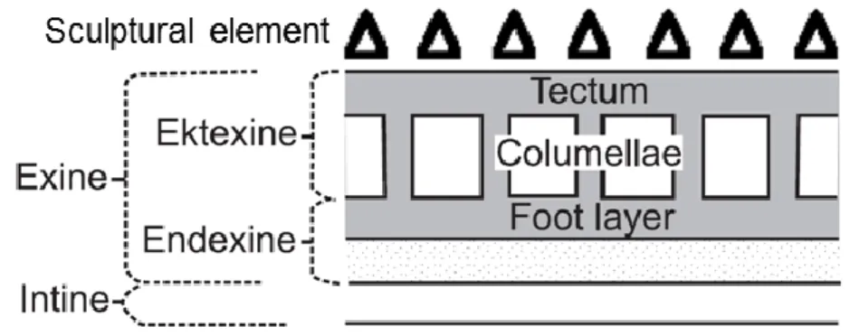
3.2.2 The main features of pollen grains ... 40
3.2.3 Dispersal and source of pollen from marine sediments ... 43
3.2.4 Pollen analysis procedure ... 44
3.3 Alkenone-derived sea surface temperature reconstruction ... 48
CHAPTER 2 The complexity of millennial-scale variability in southwestern Europe during MIS 11 Oliveira, D., Desprat, S., Rodrigues, T., Naughton, F., Hodell, D., Trigo, R., Rufino, M., Lopes, C., Abrantes, F., Sánchez Goñi, M.F. (2016) Quaternary Research 86, 373-387 Abstract ... 54
Introduction ... 55
Environmental setting and pollen signal ... 57
Material and methods IODP Site U1385 ... 59
Pollen analysis ... 59
Pollen-derived vegetation reconstruction ... 66
Long-term vegetation trends ... 66
Suborbital vegetation dynamics ... 67
Alkenone-sea surface temperature reconstruction ... 68
Discussion Long-term vegetation and climatic changes ... 72
Millennial-scale climate variability ... 74
Intra-interglacial climate variability during MIS 11c ice volume minimum ... 74
Decoupled atmospheric and oceanic changes during the glacial inception ... 77
Land-sea cooling during large ice volume conditions ... 78
Conclusions ... 81
Supplementary data ... 82
References ... 83
CHAPTER 3 Unexpected weak seasonal climate in the western Mediterranean region in response to MIS 31, a high-insolation forced interglacial Oliveira, D., Sánchez Goñi, M.F., Naughton, F., Polanco-Martínez, J.M., Jimenez-Espejo, F.J., Grimalt, J.O., Martrat, B., Voelker, A.H.L., Trigo, R., Hodell, D., Abrantes, F., Desprat, S. (2017) Quaternary Science Reviews 161, 1–17 Abstract ... 96
Introduction ... 97
Regional setting Core site and hydrographic conditions ... 99
Modern climate and vegetation ... 100
Material and methods Chronostratigraphy ... 101
Pollen analysis ... 102
Molecular biomarker analyses ... 105
Time series analysis ... 106
Results and interpretations MIS 31 definition ... 106
Pollen-based reconstruction of vegetation and climate dynamics in SW Iberia ... 107
Long-term vegetation and climate change ... 107
Astronomical factors controlling the MIS 31 vegetation and climate in SW Europe ... 118
Land - sea interaction on millennial timescales ... 120
Millennial-scale variability during glacials MIS 32 and MIS 30 ... 120
Intra-interglacial climate variability during MIS 31 ... 123
Conclusions ... 126
Supplementary data ... 128
References ... 129
CHAPTER 4 Unraveling the forcings controlling the magnitude and climate variability of the best orbital analogues for the present interglacial in SW Europe Oliveira, D., Desprat, S., Yin, Q., Naughton, F., Trigo, R., Rodrigues, T., Abrantes, F., Sánchez Goñi, M.F., under review, Climate Dynamics Abstract ... 142
Introduction ... 143
Modern setting ... 145
Material and methods Chronology ... 146
Pollen and alkenones analyses ... 147
Model and experimental setup ... 148
Results and discussion Direct land-sea comparison for MIS 1 ... 149
Interglacial intensity in the SW Iberian region ... 151
Comparing reconstructed and simulated interglacial vegetation and climate “Optima” for MIS 1, 11c and 19c ... 151
What drives the SW Iberian interglacial vegetation at the climate “Optima”? ... 157
What drives the climate variability during the Holocene and its potential analogues in SW Iberia ... 162
Conclusions ... 168
Supplementary data ... 170
SW European vegetation and climate changes during MIS 11 and MIS 31
Orbital-driven variability ... 183
Origin and diversity of millennial-scale changes ... 186
Atmospheric and oceanic cooling during large ice volume conditions ... 188
Land-sea decoupling during ice volume minimum and the glacial inception ... 189
Climatic forcings controlling the regional expression of the best orbital analogues (MIS 11c and MIS 19c) for the current interglacial in SW Europe ... 191
Main findings of the co-authored publications of relevance to the thesis ... 193
Future research and recommendations ... 195
REFERENCES for Chapters 1 and 5 ... 201
APPENDIX A Site U1385 detailed percentage pollen diagrams spanning MIS 1, MIS 11 and MIS 31 .... 221
APPENDIX B Co-authored publications of relevance to the thesis ... 227
Climate changes in south western Iberia and Mediterranean Outflow variations during two contrasting cycles of the last 1 Myrs: MIS 31–MIS 30 and MIS 12–MIS 11.
Sánchez Goñi, M.F., Llave, E., Oliveira, D., Naughton, F., Desprat, S., Ducassou, E., Hodell, D.A., Hernández-Molina, F.J. (2016) Global and Planetary Change 136, 18–29.
Dinoflagellate cyst population evolution throughout past interglacials: Key features along the Iberian margin and insights from the new IODP Site U1385 (Exp 339).
Eynaud, F., Londeix, L., Penaud, A., Sánchez Goñi, M.F., Oliveira, D., Desprat, S., Turon, J.-L. (2016). Global and Planetary Change 136, 52–64.
L’étude du pollen des séquences sédimentaires marines pour la compréhension du climat : l’exemple des périodes chaudes passée. [Pollen in marine sedimentary archives, a key for climate studies: the example of past warm periods].
RÉSUMÉ / FRENCH SUMMARY
Au cours du Quaternaire, soit les derniers 2.58 millions d’années, la Terre a connu de grands changements environnementaux se traduisant par des oscillations entre périodes glaciaires et interglaciaires. Ces oscillations qui sont cycliques sont forcées à l’origine par les variations de l’insolation, dit forçage orbital, régies par les paramètres astronomiques que sont l’excentricité, la précession et l’obliquité, qui définissent la position de la Terre par rapport au Soleil. Les interglaciaires du Quaternaire sont tous des périodes chaudes comme celle dans laquelle nous vivons, l’Holocène, durant lesquelles les calottes de glace de l’hémisphère nord sont réduites. Ils sont néanmoins très variables en termes d’intensité, de durée, de variabilité millénaire et de forçage. Certains d’entre eux présentent de fortes analogies avec le réchauffement actuel et futur et leur étude pourrait apporter des informations clés permettant de distinguer les changements climatiques « naturels » de ceux d’origine anthropique durant notre interglaciaire, et évaluer comment ce dernier pourrait évoluer en l’absence de gaz à effet de serre générés par les activités humaines.
Cette thèse est dédiée à l’étude de ces périodes interglaciaires particulières afin de documenter la réponse des composantes du système climatique telles que la cryosphère, l’océan, l’atmosphère et la biosphère ainsi que leurs interactions face à un réchauffement climatique important d’origine naturelle. Notre intérêt s’est porté sur deux stades interglaciaires en particulier, le MIS (Stade Isotopique Marin) 31, situé entre 1.082 et 1.062 ka et le MIS 11, entre 425 et 374 ka, l’un se produisant pendant la Transition du Pléistocène Moyen (MPT) alors que les cycles glaciaires-interglaciaires sont encore dominés par l’obliquité (« monde de 41-ky »), et l’autre après cette transition lorsque les cycles glaciaires-interglaciaires sont dominés par l’excentricité (« monde de 100-ky » auquel appartient aussi notre interglaciaire). Au-delà d’appartenir à un monde de variabilité climatique différent, ces deux stades présentent un forçage orbital contrasté, les variations d’insolation (et précession) pendant le MIS 11 sont faibles dues à une faible excentricité alors qu’elles sont particulièrement importantes pendant le MIS 31. Lors de ces deux interglaciaires, l’ampleur du réchauffement atteint aux hautes latitudes est pourtant similaire ; elle était telle que la dénomination de « super interglaciaire » leur a été attribuée. De plus, la fonte quasi-totale des calottes groenlandaise et ouest antarctique aurait entraîné un niveau marin bien plus élevé qu’à l’heure actuelle (Pollard and DeConto, 2009; DeConto et al., 2012;
Melles et al., 2012). Cependant, l’intensité et l’extension géographique de ce réchauffement restent sujet à débat car dans d’autres régions du globe, ces interglaciaires ne se démarquent pas des autres interglaciaires du Quaternaire, sachant tout de même que l’expression régionale du MIS 31 est à ce jour très peu connue. Par ailleurs, le MIS 11 présente un autre intérêt majeur, il est considéré avec le MIS 19 (~800 ka) comme un analogue orbital de notre interglaciaire (Yin and Berger, 2012, 2015). En effet, la configuration orbitale de la Terre pendant ces trois interglaciaires présente de fortes similitudes, se traduisant par une distribution annuelle et saisonnière de l’insolation comparable. Toutefois, le couvert forestier simulé pour les latitudes subtropicales pendant le MIS 19 (Yin and Berger, 2012) ne coïncide pas avec celui observé (Sanchez Goñi et al., 2016), ce qui indique que les mécanismes contrôlant l’expression régionale du climat durant les analogues orbitaux ne sont pas encore bien contraints.
La recherche présentée dans cette thèse a premièrement pour objectif de mieux comprendre les changements de la végétation et du climat dans le sud-ouest de l’Europe, une région subtropicale particulièrement sensible au réchauffement climatique actuel surtout en terme de disponibilité en eau, pendant les interglaciaires clés que sont les MIS 31 et MIS 11. En deuxième lieu, cette recherche s’intéresse aux forçages dominants pouvant expliquer l’intensité et la variabilité climatique de ces interglaciaires aux latitudes subtropicales. Identifier les processus responsables de la variabilité climatique des MIS 11 et MIS 31 permet une nouvelle compréhension de la nature, rapidité et causes des changements climatiques passés avec des conditions climatiques de base différentes, avant et après ~1 million d’années, i.e. les cyclicités de 41- et 100-ky. Finalement, la recherche des facteurs contrôlant le climat interglaciaires dans les subtropiques se focalisera en dernier lieu sur les analogues orbitaux de l’Holocène dans le monde de 100-ky.
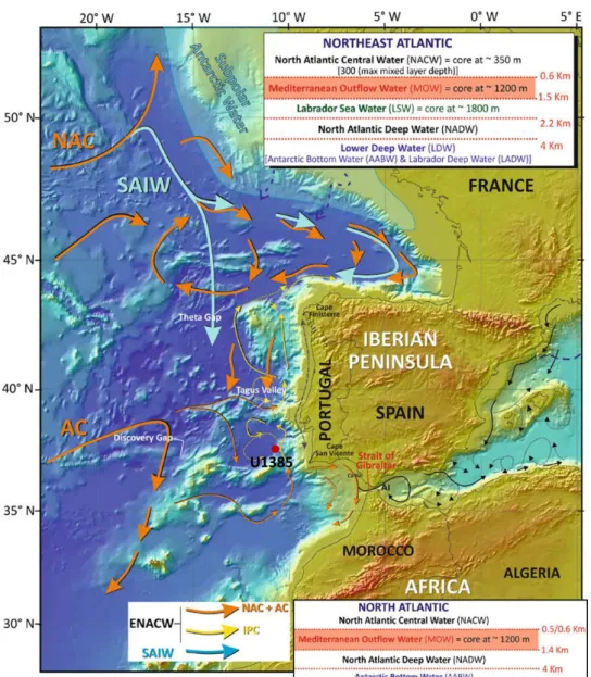
Cette thèse présente l’analyse pollinique à haute résolution (~ 400 ans) des sédiments du site IODP U1385, situé sur la marge Ibérique en face de l’estuaire du Tage, qui permet de reconstituer la végétation du proche continent, soit du sud-ouest de la péninsule Ibérique. L’analyse pollinique de sédiments marins permet de comparer directement, c’est-à-dire sans incertitudes chronologiques, les variations de la végétation régionale et du climat continental, avec celles de la température des eaux de surface de l’océan. Cette approche est donc un sérieux atout dans l’étude des réponses et interactions du système océan-atmosphère.
Les résultats majeurs obtenus à partir de l’analyse pollinique du site U1385 sont tout d’abord pour le MIS 11 (Oliveira et al., 2016, QR), une caractérisation des variations de la végétation et du climat dans le sud-ouest de l’Europe à l’échelle orbitale. Notre enregistrement pollinique reflète les trois phases classiques d’expansion de la forêt marquant une augmentation des températures et des précipitations, chacune étant associée à un minimum de précession. Néanmoins, le couvert forestier et en particulier le maquis méditerranéens restent limités au cours du MIS 11 probablement en réponse au faible forçage de la précession caractérisant ce stade. De plus, grâce à une résolution temporelle inédite, l’enregistrement pollinique du site U1385 révèle des oscillations marquées de la forêt tout au long du MIS 11, indiquant que des changements climatiques millénaires ont eu lieu quel que soit le volume de glace. La comparaison directe entre les changements océaniques et de la végétation a permis de mettre en évidence que l’amplitude et la durée des événements millénaires froids sur le continent sont variables et qu’ils ne sont pas toujours couplés à des variations de la température des eaux de surface. Nous montrons que cette diversité d’épisodes de refroidissement est le reflet des différents processus atmosphériques et océaniques en jeu dont le rôle varie en fonction des conditions limites et en particulier du volume de glace. Une configuration atmosphérique induisant la sécheresse dans le sud-ouest de la péninsule Ibérique sans changement simultané de la température des eaux de surface, ce qui rappelle le mode positif de l’Oscillation Nord-Atlantique (NAO), semble prévaloir lorsque le volume de glace est faible. Par contre, quand le volume de glace devient relativement élevé, les mécanismes associés à la dynamique des calottes glaciaires, tels que la perturbation de la circulation méridionale atlantique (AMOC) associée aux décharges d’icebergs et son impact sur les précipitations régionales, génèreraient des épisodes froids et secs de forte intensité et de longue durée dans le sud-ouest de l’Europe.
L’étude de la variabilité climatique entre 1100 et 1050 ka qui comprend le « super interglaciaire » du MIS 31 appartenant au « monte de 41-ky », révèle que malgré un forçage de la précession très important le réchauffement atmosphérique et des eaux de surface n’étaient pas exceptionnel dans cette région fortement sensible à la précession (Oliveira et al., 2017, QSR). En effet, l’enregistrement pollinique montre que cet intervalle se distingue par un régime tempéré et humide avec une saisonnalité réduite. Contrairement aux résultats obtenus pour le MIS11 (« monde de 100-ky ») qui montraient que bien que faible le forçage de la précession module le
développement de la forêt lors de ce stade, ici nous trouvons que le forçage dominant contrôlant l’expansion de la forêt tempérée est l’obliquité, ce paramètre favorisant une sécheresse estivale et un contraste saisonnier des précipitations moindres.
De plus, cette étude fournit pour la première fois des données qui montrent l’existence d’une variabilité atmosphérique millénaire pendant les MIS 31 et MIS 32 et le début du MIS 30. L’enregistrement pollinique U1385 atteste de nombreux déclins de la forêt reflétant une succession d’épisodes de refroidissement et de sècheresse prolongée dans le sud-ouest de la péninsule Ibérique. La comparaison directe continent-océan montre, comme pour le MIS 11, que l’expression des évènements de refroidissements suborbitaux est variable en fonction des conditions limites. Lorsque le volume de glace est plus élevé, c’est-à-dire, pendant les glaciaires MIS 32 et MIS 30, les événements de refroidissement se ressentent sur le continent et dans l’océan de surface et sont associés à une sècheresse marquée. Les épisodes les plus intenses, qui apparaissent comparables aux évènements de Heinrich de par leur empreinte climatique, sont probablement liés à une perturbation de l’AMOC associée à l’instabilité des calottes de glace. Au contraire, les déclins répétés de la forêt tempérée pendant le MIS 31 ne sont associés ni à des baisses de la température des eaux de surface sur la marge ibérique, ni à un forçage d’eau douce aux hautes latitudes. L’analyse statistique des séries temporelles révèle que les variations de la forêt tempérée pendant le MIS 31 sont marquées par une cyclicité de 6 000 ans. Cette cyclicité se retrouve dans l’insolation des basses latitudes en lien avec le quatrième harmonique de la précession, ce qui suggère un lien potentiel avec le forçage tropical. Ces résultats démontrent donc que dans le sud-ouest l’Europe les variations climatiques millénaires du MIS 31 sont modulées par le forçage des hautes ou des basses latitudes dont la prédominance dépend respectivement de l’état de base du climat glaciaire ou interglaciaire.
Dans sa dernière partie, cette thèse s’est concentrée sur les MIS 19, MIS 11 et MIS 1 qui sont des périodes présentant une configuration orbitale de la Terre semblable. Nous avons tout d’abord évalué la pertinence de considérer les MIS11c et MIS19c comme analogues de l’interglaciaire actuel dans le sud-ouest de l’Europe, puis nous avons cherché à déterminer les facteurs dominants qui contrôlent l’intensité de ces interglaciaires, en particulier en termes de végétation et précipitations, ainsi que l’évolution du climat au cours de ces périodes (Oliveira et al., under review, Clim. Dyn.). Pour cela, une comparaison modèle-données a été réalisée en
confrontant les simulations du climat régional obtenues avec le modèle LOVECLIM, avec les enregistrements climatiques atmosphériques et océaniques du site IODP U1385 pour les trois interglaciaires. Les expériences de modélisations utilisées sont des simulations « instantanées » des optima climatiques (au maximum d’insolation d’été dans l’hémisphère nord) et les simulations transitoires de l’intégralité de chaque période interglaciaire (insolation et CO2 variant
en fonction du temps).
Les reconstructions polliniques révèlent des divergences importantes entre l’optimum de forêt du MIS1 et ceux des MIS11c et MIS19c, ce qui remet en cause leur potentiel à être des analogues pour l’optimum climatique de notre interglaciaire dans le sud-ouest de l’Europe. Les enregistrements polliniques et les simulations climatiques suggèrent tous deux un couvert forestier plus faible au MIS11 qu’à l’Holocène probablement dû à des précipitations hivernales moindres, facteur critique pour le développement de la forêt dans notre zone d’étude. Bien que la configuration orbitale de la Terre pendant ces deux stades soit proche, l’insolation d’été et donc la température présentent un gradient latitudinal sensiblement plus important pendant l’optimum du MIS 11. Ce gradient a probablement induit une trajectoire plus méridionale des vents d’ouest, diminuant par conséquent la quantité des précipitations arrivant dans le sud-ouest de la péninsule Ibérique en hiver. Par contre, le maximum de forêt du MIS 19c indiqué par les données polliniques est substantiellement plus faible que celui reproduit par les simulations. Nous proposons que cette différence entre simulations et données est liée à la paramétrisation du volume de glace dans le modèle qui est fixé au niveau pré-industriel. En effet, les expériences de modélisation ne prennent pas en compte que le volume de glace était relativement plus important pendant le MIS 19, et notamment que la calotte glaciaire eurasiatique était plus étendue, alors que la taille et la localisation des calottes peuvent jouer un rôle important sur le parcours des tempêtes de l’Atlantique nord.
Finalement, la comparaison modèle-données de l’évolution de la végétation dans le sud-ouest de la péninsule Ibérique au cours de l’Holocène, du MIS 11c et du MIS 19c montre tout d’abord un accord entre simulations et données à l’exception notable de la déglaciation. Cette différence est attribuée au manque d’interactions entre la calotte glaciaire et le climat dans les expériences de modélisation qui incluent seulement un volume de glace typique des interglaciaires. Nous trouvons que l’expansion de la forêt dans le sud-ouest de la péninsule Ibérique est fortement corrélée avec des étés chauds et d’importantes précipitations d’hiver, ce
qui est principalement contrôlé par la précession, et que donc le CO2 joue un rôle négligeable
dans l’évolution de la forêt méditerranéenne.
Notre travail met en évidence une concordance entre variabilité millénaire intra-interglaciaire modélisée et observée dans le sud-ouest de la péninsule Ibérique, se traduisant par des réductions répétées de la forêt indiquant des épisodes de sécheresse hivernale sans diminution de la température des eaux de surface. Etant donné que les interactions calottes glaciaires-climat ont été négligées dans le modèle, les simulations transitoires mettent en évidence que le forçage astronomique à lui seul est suffisant pour produire la variabilité millénaire intra-interglaciaire observée. De plus, il est remarquable que la réduction la plus dramatique de la forêt qui a lieu à la fin de l’« optimum » de chaque interglaciaire lorsque le volume de glace est encore faible, soit aussi reproduite dans les expériences transitoires, même si elles présentent une tendance plus graduelle. Cette observation souligne le rôle potentiel de l’interaction entre les variabilités climatiques orbitale et millénaire dans l’amplification des réponses de la végétation et du climat. Néanmoins, une étude plus approfondie est clairement requise pour mieux comprendre cette interaction, ainsi que des expériences de modélisation considérant la configuration des calottes glaciaires et les rétroactions associées au sein du système climatique.
PREFACE
Over the last three million years, the Earth’s climate system underwent repeated long-term climatic shifts between cold glacial and warm interglacial periods. These long-term climate changes were originally driven by a combination of changes in precession, obliquity and eccentricity that together determine the insolation at different latitudes and the seasonal distribution. We are presently in an interglacial, the Holocene, which started about 11.700 years ago. It is widely acknowledged that the climate is changing significantly particularly so in the last few decades and that it will be warmer in the coming century (IPCC, 2013). The predicted global warming in response to anthropogenic greenhouse gases increase is accompanied by changes of other components of the climate system that will affect people and the environment worldwide, including widespread melting of ice sheets, global sea-level rise, sea-ice cover decrease and reduced global permafrost cover. As the climate of our planet appears to be heading for high rates of climate change, whether due to natural variability or human activity, a deeper knowledge of the mechanisms that drive the Earth’s climate by studying past climate changes is therefore crucial to understand the natural variability for periods stretching back beyond the instrumental record. From this perspective, it is of importance to investigate the climatic evolution of past interglacials, particularly the ones characterized by warmer climates and higher sea-levels than those of the Holocene, as they may provide decisive information about the response of the cryosphere, ocean circulation, and other components of the Earth system during our present warm climate and hopefully its future.
Marine Isotope Stage (MIS) 11 (425-374 ka), MIS 19 (790-761 ka) and MIS 31 (1.082– 1.062 ka) are periods of primary interest in this regard as they are considered among the best interglacial analogues for the current interglacial and projected global warming. The levels of warmth achieved during MIS 11 and MIS 31 were so exceptional at high latitudes that they were considered as “super interglacials” (Melles et al., 2012). However, the magnitude and geographical extent of their warming remains debatable as in other regions of the world their thermal optima do not appear warmer than that of any other interglacial of the Quaternary (the past 2.6 million years). MIS 19 in turn features a similar orbital configuration than that of the Holocene resulting in a comparable distribution of annual and seasonal temperatures (Yin and Berger, 2012, 2015). Nonetheless, there is a discrepancy between the simulated forest cover for
the subtropical latitudes (Yin and Berger, 2012) and that observed (Sanchez Goñi et al., 2016a), which highlights the interest of looking at diverse climatic variables, not only temperatures, to understand the diversity of interglacials at regional scale.
The research presented in this thesis seeks first for a better understanding of the relevant mechanisms driving the orbital and suborbital vegetation and climate changes in southwestern (SW) Europe during two different worlds: MIS 11 dominated by eccentricity (100,000-year cyclicity) and the poorly known MIS 31 dominated by obliquity (41,000-year cyclicity), respectively. Secondly it aims to unravel the forcing factors controlling the magnitude and climate variability of the Holocene and its best orbital analogues (MIS 11c and MIS 19c) in the subtropical latitudes. This is attempted by performing high resolution pollen analyses that allow a direct comparison between atmospherically-driven vegetation changes and sea surface temperature variability in the same sediment sample set from the International Ocean Discovery Program (IODP) Site U1385 (Expedition 339). This site, also known as the “Shackleton Site”, was recently collected on the SW Iberian margin, which is considered a prime location for tracking past climate changes and, additionally, has been identified as one of the most vulnerable region to the ongoing global climatic changes. Revealing the processes behind the climatic variability of MIS 11 and MIS 31 provides new insights on the nature, timing and causes of past climate changes under the different baseline climate states before and after ~1 million years, i.e. the 41,000 and 100,000-year cyclicity worlds, respectively. In addition, the discussion of Site U1385 paleoclimate records in the light of modelling experiments allows determining the dominant forcing and feedback mechanisms explaining the regional expression of the best orbital analogues of the Holocene.
In this manuscript, a number of fundamental concepts and an overview of the state-of-the-art of past interglacial climate are firstly given in Chapter 1, providing the ststate-of-the-arting point of the work presented in this thesis. To avoid repetition, this introduction does not include a detailed presentation of the current knowledge of each studied interglacial climate because this information is already provided within the three core chapters of this thesis (Chapter 2 to 4) that correspond to material published (or submitted) in peer-reviewed international journals. The main research questions of this PhD and central issues that will be addressed in Chapter 2, 3 and 4
follows the general overview. In the last part of this chapter, the study region, chronological framework and proxy-based methods are presented.
Chapter 2 focuses on the millennial-scale climate variability during MIS 11 and reveals that climate instabilities are a pervasive feature of MIS 11 in SW Europe, but most importantly it highlights the diverse expression of the cooling events in terms of magnitude, character and duration. We propose that this diversity is related to different atmospheric and oceanic configurations depending on the baseline climate states (Oliveira et al., 2016, QR).
Chapter 3 presents the first direct comparison between oceanic and atmospherically-driven vegetation changes in SW Iberian region between MIS 32 and early MIS 30, including the MIS 31. We show that, despite its extreme precession forcing, MIS 31 was characterized by a temperate and humid climate regime marked by weak seasonality in this region very sensitive to precession during the 100,000-year world. We find that this regional signature was likely due to the prevailing influence of obliquity in controlling the hydroclimate of subtropical latitudes. In addition, this study reveals that the different expression of the climatic instabilities during the glacials and MIS 31 interglacial probably reflect the predominance of high or low-latitude forcing, respectively, on the SW European climate variability (Oliveira et al., 2017, QSR).
In Chapter 4, we examine the vegetation and climate features of the best orbital analogues of the Holocene, i.e. MIS 11c and MIS 19c, in SW Europe and we seek to determine the controlling factors responsible for their regional climatic expression. For that, we used a model-data comparison based on snapshot and transient experiments performed with the LOVECLIM climate model and new and published terrestrial-marine climate profiles from Site U1385 (Holocene: Chapter 4, MIS 11c: Oliveira et al., 2016 and MIS 19c: Sánchez Goñi et al., 2016a). We show that MIS 11c and MIS 19c cannot be considered as straightforward analogues of the Holocene climate “optimum”, which was characterized by a much larger forest extent. Our model-data comparison reveals that the differences between the three interglacial peaks and throughout the interglacials were primarily constrained by the winter hydroclimate which is in turn mainly controlled by precession whereas CO2 played a negligible role in the subtropics
forest development. Moreover, we find that the observed intra-interglacial variability and the strong forest reductions marking the end of the interglacial “optimum” is well reproduced in
climate simulations. This finding underlies the potential role of the interactions between long-term and millennial-scale climate dynamics in amplifying the climate and vegetation response (Oliveira et al., under review, Climate Dynamics).
Finally, the main conclusions and future perspectives are summarized in Chapter 5 followed by Appendix A, including the detailed percentage pollen diagrams for MIS 1, MIS 11 and MIS 31, and Appendix B presenting additional publications to which I have substantially contributed.
Chapter 1
1. INTERGLACIAL CLIMATES
1.1 Fundamental concepts and general overview
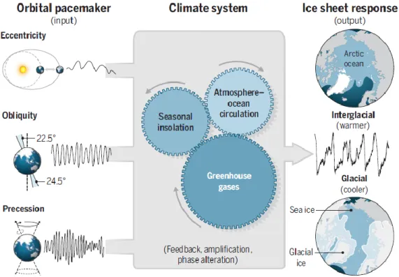
During the Quaternary, global climate has repeatedly changed between cold glacial and warm interglacial conditions primarily due to gradual variations in insolation (e.g. Milankovitch, 1920; Shackleton and Opdyke, 1973; Berger, 1975; Hays et al., 1976; Imbrie et al., 1992; Berger and Loutre, 1994; Ruddiman, 2006). Changes in the amount of incoming solar radiation (insolation) as well as its seasonal and latitudinal distribution are controlled by oscillations in the Earth’s orbital geometry modulated by three orbital parameters as first established by Milutin Milankovitch (Milankovitch, 1920, 1941) (Fig. 1):
(1) Eccentricity reflects the shape of Earth's orbit around the Sun, ranging from a quasi-circular (low eccentricity of 0.0006) to a slightly elliptical shape (high eccentricity of 0.0535) and with two periodicities of about 100 and 400 thousands of years (hereafter ky) (Berger and Loutre, 1992; Berger and Loutre, 2004). The eccentricity is the only parameter that changes the mean insolation received globally and annually by the Earth (Berger, 1975).
(2) Obliquity refers to the tilt of Earth’s rotation axis relative to a perpendicular to the orbital plane, varying from 22° to 24.5° (current value of ~23.5°) with a periodicity of about 41 ky (Berger and Loutre, 2004). It determines the distribution of insolation between the summer and winter season with a symmetric impact in both hemispheres. Fluctuations in obliquity have less influence at low-latitudes as the strength of its effect decline towards the equator (e.g. Buchdahl, 1999; Berger et al., 2010).
(3) Precession of the equinoxes (change in the orientation of the Earth's rotational axis) is modulated by eccentricity, which splits the precession into two periods of about 23 ky and 19 ky, leading to an average period of 21 ky (Berger, 2001; Berger and Loutre, 2004). This cycle has two components: an axial precession, caused by the gravitational forces exerted on Earth of all other planetary bodies in our solar system, and an elliptical precession, in which the elliptical orbit of the Earth itself rotates about one focus (Buchdahl, 1999). Changes in axial precession modify the times of perihelion and aphelion, and consequently increase the seasonal contrast in one hemisphere and decrease in the other hemisphere. The hemisphere at perihelion experiences an increase in summer solar radiation and a cooler winter, while the opposite hemisphere will have a warmer winter and a cooler summer. Presently, the Earth is
at perihelion in the northern hemisphere (hereafter NH) winter, which makes the winters and summers less severe in this region (Ruddiman, 2001).
The changes in orbital forcing drove the growth and decay of glaciers that together with other feedback processes (e.g. greenhouse gases (GHG), albedo) gave rise to glacial-interglacial (G-I) cycles (Fig. 1). These cycles were clearly observed not only in the records of benthic foraminifera oxygen isotope ratio (δ18O) (e.g. Emiliani, 1955; Shackleton and Opdyke, 1973; Hays et al., 1976; Lisiecki and Raymo, 2005) but also in an extensive range of marine, ice core, lacustrine and terrestrial archives all around the world. Shackleton (1967) demonstrated, based on the δ18O of benthic foraminifera curve from a deep-sea core covering
the last 1 million years (hereafter My), the occurrence of ice volume changes producing long periods of glacial climates during which extensive ice sheets developed (heavy δ18O values) separated by temperate/warm conditions with restricted ice sheets extent (light δ18O values).
The δ18O records were later used for stratigraphic purpose and divided into numbered marine
isotope stages (MIS; G-I corresponding to even- and odd-numbers, respectively, excepting MIS 3 which is a part of the last glacial period) (Shackleton and Opdyke, 1973). Over the past decades, the chronostratigraphic framework of the Quaternary has been gradually improved based on orbitally tuned δ18O-stack records (e.g. Imbrie et al., 1984; Martinson et al., 1987;
Shackleton et al., 1990; Bassinot et al., 1994; Lisiecki and Raymo, 2005). Correlating individual benthic profiles with a global stack, such as the LR04, is a common practice to establish a chronological framework for long marine sedimentary records. However, local deep-water temperatures and hydrography can also influence benthic δ18O signals predominantly used as an indicator of global ice volume (Skinner and Shackleton, 2005). In addition, a recent work shows that global stacks neglect regional differences that can reach several thousands of years during glacial terminations possibly causing significant deviations (Lisiecki and Stern, 2016). Regional δ18O stacks may, therefore, provide a better stratigraphic
alignment targets than the LR04 global stack, which is older by 1-2 ky throughout the Pleistocene according to these new regional δ18O tuning targets (Lisiecki and Stern, 2016).
The orbital-scale variability within the MIS may be further divided into interstadials and stadials representing secondary advances or retreats of glaciers, which are referred by the stage number followed by a substage letter (e.g. Shackleton, 1969) or number (e.g. Bassinot et al., 1994). Since the MIS substage and decimal event notation are not interchangeable, as substages refer to intervals and oxygen isotope events refer to individual points in time, a
complete and optimized scheme of substage nomenclature for the last one million years was recently proposed by Railsback et al. (2015) for use henceforth in palaeoclimate studies.
Fig. 1. Schematic representation of the “Pacemaker of the ice ages” mechanism of Hays,
Imbrie and Shackleton (1976) that provided strong support for the Milankovitch hypothesis (from Hodell, 2016). In the pacemaker analogy, the pacemaker is the cyclic variations in Earth’s orbital geometry, the heart is the climate system, and the heartbeat is the resulting G-I cycles.
It is important to note that as shown by the combination of pollen and isotope analyses in marine sediments, the ice volume and vegetation changes did not occur necessarily simultaneously (for example, regional forest conditions persisted during some intervals of northern hemisphere ice growth) (e.g. Sánchez Goñi et al., 1999; Shackleton et al., 2002, 2003). Therefore, the marine and terrestrial stage boundaries are generally not isochronous. It is also extremely important to note that the term “MIS” and “interglacial complex” is not synonymous with the term interglacial (e.g. Shackleton, 1969; Martinson et al., 1987; Tzedakis et al., 2009a). The term “interglacial” was initially developed based on pollen stratigraphy in western and central Europe and North America to refer to a climate episode at least as warm as the Holocene that allowed the expansion of temperate deciduous forest (e.g. Fairbridge, 1972; Turner, 1970; West, 1984; Gibbard and West, 2000). However, the term “interglacial” has been loosely defined due to the large number of different approaches and criteria used. A review by the Past Interglacials working group of PAGES (2016) recently
forward a working definition of interglacial for the last 800 ky that may be more objectively applied. Based on sea-level close to present, an interglacial would correspond to the interval of minima continental ice volume with a distribution of NH ice similar to the present (0 ± 20 m), i.e. there was litle NH ice outside Greenland, with periods of higher ice volume (~ 50 m below present sea-level) before and after the interglacial period (Past Interglacials working group of PAGES, 2016). This often ends up with the interglacial being the MIS substage after deglaciation, as observed by isotopic minimum, sea-level high stand and/or less positive seawater δ18O. However, the paucity of archives that are currently available hamper the
validation of this working definition and, therefore, an accurate and consistent identification of the interglacials intervals (Past Interglacials working group of PAGES, 2016). For simplicity's sake throughout this thesis the term interglacial is generally used to refer to the interglacial complex, i.e. the MIS, while the interglacial as defined by Past Interglacials working group of PAGES (2016) is referred to as the respective lightest δ18O MIS substage (e.g. MIS 5e, 9e, 11c, 19c).
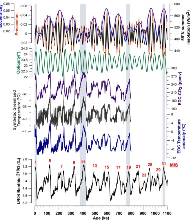
Despite the large number of studies that exists regarding the orbital variability described by Milankovitch, there is still an extensive debate about the exact contribution of orbital parameters in modulating the Earth’s climate, particularly during the Mid Pleistocene Transition (MPT, 1.25-0.7 Ma, Clark et al., 2006), more recently known as the Early Middle Pleistocene Transition (Head and Gibbard, 2015). During this enigmatic transition, the Earth’s climate underwent prominent changes in G-I amplitude and periodicity, from dominant symmetrical low-amplitude and high-frequency (41 ky obliquity-driven) climate cycles prior to ∼900 ky to increasing long-term average global ice volume and dominant asymmetrical high amplitude and low-frequency (100 ky eccentricity-forced) climate cycles (Fig. 2), under no significant difference in the orbital forcing (e.g. Pisias and Moore, 1981; Lisiecki and Raymo, 2005; Clark et al., 2006; Elderfield et al., 2012; Head and Gibbard, 2015). The exact timing of deglaciations and glaciations, role of orbital forcing and mechanisms of the onset of the 100-ky periodicity represents a major challenge in the palaeoclimate research (Huybers 2007, 2011; Maslin and Brierley, 2015 and references therein; Tzedakis et al., 2017). Various internal processes such as ice sheet size and configuration, GHG, ocean and atmospheric dynamics and vegetation were invoked to explain the observed changes during the MPT.
Fig. 2. Orbitally-driven 100-ky and 41-ky climatic oscillations. The North Atlantic benthic
foraminiferal δ18O record shows a general cooling trend in global climate together with an
increase in global ice volume over the past 3 My (diagonal white line). The G-I variability changed from symmetrical low-amplitude variations during the early Pleistocene (the “41-ky world”) to high-amplitude asymmetrical variations during the middle-to late Pleistocene (the “100-ky world”). MPT: Mid Pleistocene Transition. (from Ruddiman, 2001).
Interglacial climate variability over the MPT has received little attention mainly due to the scarcity of palaeoclimatic records available for this interval (Head and Gibbard, 2015 and references therein). Within the MPT, MIS 31 (~1.07 Ma) stands out as a long lasting interglacial marked by exceptional warmth in the high-latitude records (e.g. Scherer et al., 2008; DeConto et al., 2012; Melles et al., 2012; de Wet et al., 2016). The typical configuration of the ~ 100-ky G-I cycles initiates at MIS 25 (~0.95 Ma), with higher G-I contrasts occurring after this interglacial (e.g. Wright and Flower, 2002; McClymont et al., 2008; Hernández-Almeida et al., 2012, 2013). High-resolution records in the subpolar gyre (IODP Site U1314) between MIS 31 and MIS 19 provide evidence for warmer interglacials temperatures after MIS 25 and larger oscillations in the position of the Arctic Front (Hernández-Almeida et al., 2012, 2013). It is suggested that these oscillations allowed increased northward export of heat and moisture during interglacials, with MIS 21 and MIS
19 displaying substantial northward retreat of the Arctic Front, which favoured the buildup of larger ice sheets during the glacials of the MPT (Ruddiman and McIntyre, 1981; Raymo and Nisancioglu, 2003; Hernández-Almeida et al., 2013). MIS 23 is generally noted as the weakest interglacial of the MPT and interrupts the interval from MIS 24 to MIS 22 (936-866 ka), the “900 ka event” (Clark et al., 2006), marking the first long-duration glaciation of the Pleistocene and a progression to the heaviest δ18O values of the MPT (e.g. Weirauch et al., 2008; Elderfield et al., 2012). In SW Europe, the small number of available pollen-based vegetation and climate reconstructions that cover the MPT lack the chronological precision and/or required time resolution to investigate in detail the regional interglacial climate variability and its relationship with records of North Atlantic (Tzedakis et al., 2006 and references therein). Yet, on the well-known Tenaghi Philippon sequence, spanning the last 1.35 My, Tzedakis et al. (2006) found that both the obliquity and precession signals persisted into the 100- and 41-kyr worlds, respectively. Other low-resolution SW European pollen studies also provide evidence of both obliquity and precession-driven changes before and across the MPT, highlighting the pervasive influence of precession on the Mediterranean climate, including during the 41-ky world (Joannin et al., 2007, 2008, 2011; Tzedakis 2007 and references therein).
During the last ~800 ky, global climate was dominated by the regular 100-ky driven symmetrical “saw-tooth” pattern of G-I changes (Fig. 2) resulting from a non-linear response of the climate system to orbital forcing (e.g. Hays et al., 1976; Imbrie et al., 1992). This time interval is well represented in marine and terrestrial sequences from a range of locations across the globe and has received a large amount of attention since the recovery of the long Antarctic ice core EPICA Dome C which extends back eight glacial cycles (~last 740 ky) (see Past Interglacials working group of PAGES, 2016 for a recent review). In addition, this period has also been the target of Earth models of intermediate complexity (EMICs) which are focused on several climate cycles and those of full Earth system models (ESMs) that consider varying boundary conditions, including the ones of recent interglacials (e.g. Yin and Berger, 2010, 2012, 2015; Ganopolski and Robinson, 2011; Herold et al., 2012; Bakker et al., 2013, 2014; Milker et al., 2013; Yin, 2013; Capron et al., 2014; Kleinen et al., 2014, 2016; Ganopolski et al., 2016).
Using the LOVECLIM model, Yin and Berger (2010, 2012, 2015) have investigated, the individual contributions of the primary forcings (insolation and GHG) to different climate-related parameters (temperature, tree fraction, sea ice) of the interglacials at the climate “optimum” and also across the entire period of each interglacial. They have found that: a) there is not a straightforward relationship between astronomical forcing and the interglacial intensity, which is not directly related to the closest precession peak or the phase of obliquity maximum and precession minimum; b) the warmest, MIS 5e and MIS 9e, and coolest, MIS 13 and MIS 17 in the high-latitudes results of the combined contribution of insolation and GHG; c) insolation (peak in boreal summer insolation) plays a dominant role on the variation of the tree fraction globally and precipitation, and in particular the North African (southern Mediterranean) tree fraction is highly correlated with precession, with GHG playing a negligible role, d) even if MIS 11 and MIS 19 are considered as the best analogues for the Holocene from an astronomical point of view, they do not show the same variations of annual and seasonal temperatures under the combined effect of the primary forcings. The major difference for MIS 11 is related to its higher GHG concentration and a slightly different insolation pattern (Ganopolski et al., 2016), which leads to a warmer interglacial than that of the Holocene and MIS 19c.
In agreement with data compilations from Lang and Wolff (2011) and Past Interglacials working group of PAGES (2016), Yin and Berger simulations (2012, 2015) also show a strong regional variability in the intensity of interglacial periods across the last 800 ky. In contrast to high-latitude locations, simulated temperatures in southern Europe appear comparable for all interglacials. Nevertheless, the tree fraction in the subtropics is simulated as highly variable from one interglacial to another, which highlights the importance of evaluating precipitation when assessing the regional expression of interglacials in lower latitudes (Yin and Berger, 2012, 2015). These model results are in line with a recent composite SST record showing that the interglacials over the last ~1 My off the Iberian Margin were characterized by similar levels of warmth with SST close to 20ºC (Rodrigues et al., 2016). However, one should keep in mind that the interglacial intensity and its regional expression have been routinely evaluated in terms of thermal regime with little attention paid to precipitation patterns. In regions with landscapes and ecosystems highly susceptible to hydrological changes, such as the Mediterranean, it is therefore crucial to consider precipitation changes. The Mediterranean region, including the SW Iberian Peninsula, has been identified as one of the most vulnerable regions to global warming (Giorgi, 2006).
Climate projections show repeated occurrence of severe drought episodes and a reduction of the mean annual precipitation in the Mediterranean area that will deeply affect the natural landscape systems (Gao and Giorgi, 2008; Solomon et al., 2009; Anav and Mariotti, 2011; Santini et al., 2014; Sousa et al., 2015; Guiot and Cramer, 2016). Future climate changes in the Mediterranean region may lead for example to the expansion of temperate evergreen broadleaved trees in zones previously occupied by temperate deciduous trees and to the collapse of the Mediterranean forest in drier zones (Anav and Mariotti, 2011; Santini et al., 2014). Yet, important biases are found in models used for simulating the Mediterranean climate and ecosystem responses to global climate change (Gao and Giorgi, 2008), which emphasizes the need to integrate proxy-based climate reconstructions in model experiments (Flato et al., 2013).
Another subject of debate in the interglacial climate research of the last 800 ky lies in the presence/absence of differences between the post-MBE (MBE: mid-Brunhes Event, between MIS 13 and MIS 11) and the pre-MBE interglacials (Yin and Berger, 2010; Lang and Wolff, 2011; Candy and McClymont, 2013; Past Interglacials working group of PAGES, 2016). Interglacial periods before this event appeared to be long and characterized by larger ice sheets, lower sea-level, cooler temperatures in Antarctica and reduced CO2 than the more
recent ones (e.g. Lambeck et al., 2002; EPICA, 2004; Bintanja et al., 2005; Lisiecki and Raymo 2005; Lüthi et al., 2008). However the expression of the MBE was neither globally or regionally uniform (Candy and McClymont, 2013; Past Interglacials working group of PAGES, 2016), being only clearly expressed in climatic variables dominated by GHG such as global annual mean temperature, but not in the ones dominated by insolation such as tree fraction and precipitation (Yin and Berger, 2010, 2012).
As far as the length of interglacials is concerned, interglacials have an overall duration ranging between ~10 and 30 ky consistent with orbital forcing timescale, with MIS 7e and MIS 11c being generally the shortest and longest, respectively (Past Interglacials working group of PAGES, 2016). Tzedakis et al. (2012a) suggested that the phasing of precession and obliquity played an important role in the persistence of interglacial conditions over one or two insolation peaks, leading to short (~13 ± 3 ky, MIS 5e, 7e, 9e, 15a and 19c) or long (~28 ± 2 ky, MIS 11c, 13a and 17) interglacials. However, estimating the interglacial duration remains problematic as it is based on the definition and identification of the interglacial onset and termination (Tzedakis et al., 2012a, b). Recently, a simple rule has been proposed based on