HAL Id: hal-00302791
https://hal.archives-ouvertes.fr/hal-00302791
Submitted on 17 Oct 2006
HAL is a multi-disciplinary open access
archive for the deposit and dissemination of
sci-entific research documents, whether they are
pub-lished or not. The documents may come from
teaching and research institutions in France or
abroad, or from public or private research centers.
L’archive ouverte pluridisciplinaire HAL, est
destinée au dépôt et à la diffusion de documents
scientifiques de niveau recherche, publiés ou non,
émanant des établissements d’enseignement et de
recherche français ou étrangers, des laboratoires
publics ou privés.
Nonlinear correlations of daily temperature records over
land
I. Bartos, I. M. Jánosi
To cite this version:
I. Bartos, I. M. Jánosi. Nonlinear correlations of daily temperature records over land. Nonlinear
Processes in Geophysics, European Geosciences Union (EGU), 2006, 13 (5), pp.571-576. �hal-00302791�
www.nonlin-processes-geophys.net/13/571/2006/ © Author(s) 2006. This work is licensed
under a Creative Commons License.
Nonlinear Processes
in Geophysics
Nonlinear correlations of daily temperature records over land
I. Bartos and I. M. J´anosi
Department of Physics of Complex Systems, E¨otv¨os University, Budapest, Hungary
Received: 21 August 2006 – Revised: 13 October 2006 – Accepted: 14 October 2006 – Published: 17 October 2006
Abstract. We present a near global statistics on the
correla-tion properties of daily temperature records. Data from ter-restrial meteorological stations in the Global Daily Climatol-ogy Network are analyzed by means of detrended fluctuation analysis. Long-range temporal correlations extending up to several years are detected for each station. In order to reveal nonlinearity, we evaluated the magnitude of daily tempera-ture changes (volatility) by the same method. The results clearly indicate the presence of nonlinearities in temperature time series, furthemore the geographic distribution of corre-lation exponents exhibits well defined clustering.
1 Introduction
The time evolution of weather or climate is conveniently characterized by its memory. Short-term memory of a dy-namical system is associated with a finite integral timescale ensuing from an exponential decay of the autocorrelation function (von Storch and Zwiers, 1999). Long-term mem-ory is characterized by a diverging integral timescale and linked to power-law behavior of the autocorrelation func-tion (Fraedrich, 2003). Irrespective of the funcfunc-tional form, 2-point correlations reveal only one aspect of the tempo-ral complexity. In genetempo-ral, higher order statistics would be needed to fully characterize the statistical properties of a dy-namical system (Mendel, 1991).
When higher order (3-point, 4-point, ...) correlations are trivially related to the 2-point correlation function, the process is termed “linear” and “monofractal”. In case of a nontrivial relationship, the process is called “nonlinear” and “multifractal” (Kalisky et al., 2005). Instead of the rather complicated direct methods for higher order statistics, Ashkenazy et al. (2001) suggested a simple measure for non-Correspondence to: I. M. J´anosi
(janosi@lecso.elte.hu)
linearity of a time series: when the magnitude of increment series (called volatility) obeys nontrivial long-range correla-tion, the original time series is nonlinear.
Besides biomedical (Ashkenazy et al., 2001; Kantelhardt et al., 2002) or hydrological (Livina et al., 2003) applica-tions, the evaluation of volatility correlations is widely used in econometric time series (Liu et al., 1999; Qiu et al., 2006). It has been recognized quite a time that the magnitudes of price changes exhibit long-range correlations, reflecting the fact that economic markets experience quiet periods with clusters of less pronounced price fluctuations, followed by more volatile periods with pronounced jumps up and down. A similar behavior for temperature records was detected too (Govindan et al., 2003), even on a paleoclimatic time scale (Ashkenazy et al., 2003), or deep in the equatorial Pa-cific (Kalisky et al., 2005). A fundamental difference be-tween econometric and temperature records is that the prices themselves are uncorrelated having a white noise spectrum, in contrast temperature data exhibit long-range correlations (Pelletier, 1997; Koscielny-Bunde et al., 1998; Talkner and Weber, 2000; Kantelhardt et al., 2001; Weber and Talkner, 2001; Kir´aly and J´anosi, 2002; Blender and Fraedrich, 2003; Fraedrich, 2003; Fraedrich and Blender, 2003; Fraedrich et al., 2003; Pattanty´us- ´Abrah´am et al., 2004; Kir´aly and J´anosi, 2005; Kir´aly et al., 2006).
In this paper we provide an analysis of correlation prop-erties for surface temperature data on a nearly global scale. We use the method of detrended fluctuation analysis (Peng et al., 1994, 1995), which became widely accepted in the past years mostly because of its capability of treating nonsta-tionary signals. We show that temperature volatility records obey asymptotic correlations for most of the stations. The geographic distribution of scaling exponents exhibits definite spatial correlations.
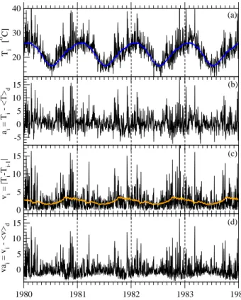
572 I. Bartos and I. M. J´anosi: Nonlinear correlations of daily temperature records 20 30 40 Ti [ o C] -5 0 5 10 15 ai = T i - <T> d 0 5 10 15 vi = |T i -T i-1 | 1980 1981 1982 1983 1984 0 5 10 15 va i = v i - <v> d (a) (b) (c) (d)
Fig. 1. Example time series evaluated in this work: Sydney station
(Australia), 33.87◦S, 151.20◦E. (a) Four years (out of the 138) of daily maximum temperatures (black) with the empirical annual cy-cle (blue). (b) Daily maximum temperature-anomaly time series.
(c) Volatility series with the empirical annual cycle (orange). (d)
Volatility-anomaly series.
2 Data and methods
We evaluated daily minimum and maximum tempera-ture records from the Global Daily Climatology Network (GDCN – http://www.ncdc.noaa.gov/oa/climate/re-search/ gdcn/gdcn.html). We concentrated our analysis on the 7320 stations (out of the total 14 737) where the number of recorded data exceeds 8000 (approximately 22 years) with less then 1% missing intervals. Since daily minima and max-ima show very similar correlation properties (Kir´aly et al., 2006), we present results for maximum values only.
As a first step of the analysis, the annual periodicity is re-moved from the daily temperature values Ti (Fig. 1a) by the long-time climatological mean hT id for the given calendar day d=1. . .366 (when leap days are included), as usual. Note that this procedure, which provides the temperature-anomaly data ai=Ti− hT id(Fig. 1b), cannot remove slow trends from the original time series, such as a gradual shift of the an-nual means. The volatility is defined as the absolute value of temperature-anomaly difference or temperature difference
vi=|ai−ai−1|≈|Ti−Ti−1|. The two definitions give practi-cally the same numerical values, because the deviation of
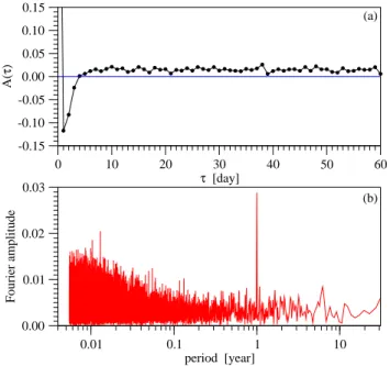
0 0.1 0.2 0.3 0.4 0.01 0.1 1 10 period [year] 0 0.02 0.04 0.06 Fourier amplitude (a) (b)
Fig. 2. The high frequency part of the power spectrum as a
func-tion of period for (a) the volatility series shown in Fig. 1c, and (b) the volatility-anomaly series shown in Fig. 1d. Note the different vertical scales. The horizontal axes are logarithmic.
climatological averages for consecutive days is typically less than the resolution of temperature data (0.1◦C). The volatil-ity series shown in Fig. 1c clearly exhibits a residual annual periodicity as a consequence of seasonally changing variabil-ity, which is a well-known attribute of extratropical climate. Figure 1d shows the volatility-anomaly series vai=vi−hvid, produced by subtracting the climatological mean values from the signal, as above. At first sight, the removal of annual periodicity might seem to be unsuccessful, however stan-dard Fourier tests (Fig. 2) demonstrate convincingly that the volatility-anomaly series do not have residual periodicities. (Note that the vertical scale in Fig. 2a is six times larger than in Fig. 2b.) Alternatively, the annual component can be removed by normalization with the climatological mean values: va0i=vi/hvid. Such series have positive sign every-where and strongly suppressed magnitudes compared to vai, nevertheless the correlation properties reflected in the Fourier spectra or DFA scaling (see below) are fully equivalent.
Next we consider the anomaly series as increments of a random walk process. The “trajectory” or “profile” of the signal xi is given by simple summation as yj=Pji=1xi, here xi denotes either ai or vai. We divide the profile into nonoverlapping segments of equal length n. In each seg-ment, the local trend is fitted by a polynomial of order p and the profile is detrended by subtracting this local fit. The usual measure of fluctuations is the standard deviation of the detrended segment averaged over all the segments hFp(n)i. A power-law relationship between hFp(n)iand n indicates scaling with an exponent δ (DFAp exponent):
hFp(n)i ∼ nδ . (1)
1 2 3 4 log10(n) 0 0.5 1 1.5 2 2.5 log 10 [F(n)] Sydney Tmax surrogated 1 2 3 4 log10(n) 0 0.5 1 1.5 2 Sydney volatility from surrogated Tmax
(a) (b)
δ = 0.65 δvol = 0.61
Fig. 3. DFA2 curves for the signals shown in Fig. 1. (a) Daily
maximum temperature-anomalies (yellow circles) and its surrogate (black diamonds). The latter is produced by an iterative inverse Fourier algorithm matching the autocorrelation functions and prob-ability distributions (see text). (b) Volatility-anomalies (yellow cir-cles) and the volatility-anomalies obtained from the surrogate tem-perature record (black diamonds). Dashed lines illustrate a slope of 1/2 (uncorrelated processes), exponent values are indicated.
Notice that such a process has power-law autocorrelation function and power spectrum
A(τ ) = haiai+τi ∼τ−α , S(f ) ∼ f−β , (2) where stationarity requires 0<α<1 and 0<β<1. The rela-tionships between the correlation exponents are (Koscielny-Bunde et al., 1998; Talkner and Weber, 2000)
α =2(1 − δ) , β =2δ − 1 . (3)
Processes of long-term memory are characterized by DFA exponents δ>1/2, uncorrelated time series (e.g., pure rdom walk) obey δ=1/2. Signals with δ<1/2 are called an-tipersistent, expressing the tendency that an increasing trend in the past implies a decreasing trend in the future, and vice versa.
Local polynomial fits of order p eliminate polynomial background trends of order p−1. In practice, long-term cor-relation is inferred when the exponent δ does not depend on p.
Figure 3 illustrates results for the Sydney station. Since we observed slope differences between DFA1 and DFA2 curves for a few stations but not between DFA2, DFA3 and DFA4 within the numerical accuracy of the fitting procedure, we performed the overall evaluation by second order local de-trending (DFA2). Exponent values were obtained by linear fits in the interval [30, 2000] days (log10(n) ∈ [1.47, 3.30]).
In order to demonstrate that long-range correlation in the volatility-anomaly series is indeed a consequence of higher order (nonlinear) correlations, we implemented the method of data surrogation by Schreiber and Schmitz (2000). (For technical details see: Hegger et al., 1999). This proce-dure does not affect 2-point correlations, whatever is their nature (short-term or long-term), but effectively destroys
0.5 0.6 0.7 0.8 0.9 δ 0.1 1 10 Normalized frequency 0.5 0.6 0.7 0.8 0.9 δvol (a) (b)
Fig. 4. Normalized histogram of asymptotic DFA2 exponents for (a) daily maximum temperature-anomalies, and (b) volatility-anomalies. Statistics for 7320 stations is shown.
higher order correlations in the series. The DFA2 curve of volatility-anomaly series obtained from the surrogate tem-perature record (Fig. 3b, black diamonds) clearly indicates the lack of long-range correlations, while the surrogate se-ries itself has the same 2-point correlation behavior (Fig. 3a).
3 Results
Figure 4 shows the overall statistics of DFA2 exponents for the analyzed stations. Since exponent values could be ob-tained with a numerical accuracy of ±0.05 (see also: Kir´aly et al., 2006), we conclude that daily temperature anomalies obey significant long-term correlations everywhere. The his-togram of volatility-anomaly exponents δvol(Fig. 4b) is nar-rower, significant scaling behavior (δvol>0.55) can be de-clared for 6526 stations (89%) out of the total 7320.
The geographic distribution of exponent values is shown in Fig. 5. Unfortunately South-America and Africa are strongly underrepresented in the GDCN data base, furthermore the spatial coverage is very uneven (Kir´aly et al., 2006). Never-theless it seems that relatively low δ values are characteristic at the south-eastern continental boundaries (Fig. 5a). As for the volatility exponents δvol, the geographic pattern is quite different (Fig. 5b). Probably the only solid conclusion which can be drawn is the tendency of clustering: there are rela-tively large areas where the exponent values for neighboring stations are similar. This suggests that the results are not nu-merical artefacts, but they can have a climatological origin.
The comparison of maps in Figs. 5a and b already suggests that there is no strong correlation between the exponent val-ues δ and δvolfor individual stations. The scatter plot shown in Fig. 6 confirms completely this suspicion.
The original observations on a possible link between non-linearity and long-range volatility correlations (Ashkenazy et al., 2001) were fully empirical. Later, Kalisky et al. (2005) and Jun et al. (2006) have developed analytical tools to estab-lish relations between the scaling exponents of a time series
574 I. Bartos and I. M. J´anosi: Nonlinear correlations of daily temperature records
(b)
(a)
Fig. 5. Geographic distribution of asymptotic DFA2 exponent
val-ues for 7320 stations. (a) δ for daily maximum temperature anoma-lies. (b) δvolfor volatility anomalies. (The color scale is nonlinear
and codes different intervals for the two cases.)
and its volatility. In Fig. 6 we show a comparison with the predictions of Kalisky et al. (2005). The black dashed line in-dicates the expected behavior for a linear process, where the 2-point correlations obey a power law with DFA exponent δ. Up to the value δ≈0.75, the volatility exponent is practically constant δvol=0.5, and then changes to an approximately linear increase. Unfortunately the number of stations with the strong correlation δ>0.75 is quite limited, c.f. Fig. 4a, thus the possible crossover in the empirical data is not clear enough. Nevertheless we can probably reject the hypothe-sis that the temperature records can be fully represented by linear processes with 2-point (power-law) correlations only.
The blue line in Fig. 6 shows the predictions for multifrac-tal processes with a parameter σ =0.05, which characterizes the width of the multifractal spectra (Kalisky et al., 2005). The red cloud of the scatter plot does not follow this pre-diction neither, but at least the blue line crosses its center. One possible explanation of the unstructured scatter plot in Fig. 6 can be that the numerical differentiation used to pro-duce volatility series is known to strongly enhance inherent noise level in the data, therefore the weak dependence of δvol on δ remains hidden.
In the original proposal, Ashkenazy et al. (2001) decom-posed the derivatives of the time series into a volatility and a sign series. The latter is formed by assigning +1 when the one-day difference Ti−Ti−1is positive, and −1 when it is negative. We evaluated the sign series for daily maximum
0.5 0.6 0.7 0.8 0.9 1
δ
0.45 0.5 0.55 0.6 0.65 0.7 0.75δ
volFig. 6. Correlation plot for the temperature anomaly exponent (δ) and volatility anomaly exponent (δvol) for each station. Black
dashed line indicates the theoretical prediction by Kalisky et al. (2005) for long-range correlated linear processes, the blue line is the same for multifractal series with the parameter σ =0.05.
temperatures as well, but we did not find nontrivial results. Figure 7 reveals that the sign of temperature changes can have a weak anticorrelation for time lags up to 4 days, and a clear annual periodicity reflecting the seasonal changes. Oth-erwise the sign series are uncorrelated. The DFA method is not really suitable to analyze such series, because the typi-cal magnitude of fluctuations around the lotypi-cal trends is ex-tremely small.
4 Conclusions
Although the application of detrended fluctuation analysis has its own pitfalls (Metzler, 2003; Maraun et al., 2004), we can conclude with low risk that terrestrial temperature records obey long-range nonlinear correlations. The term “long-range correlation” obviously does not mean an infinite memory, it reflects simply the fact that we did not observe any breakdown of empirical DFA curves in the available time intervals for temperature anomaly and volatility signals with-out annual periodicities (c.f. Fig. 3). Indeed, Blender and Fraedrich (2003) and Fraedrich and Blender (2003) demon-strated by globally coupled models that the scaling regime might be restricted, and correlations fade away over ∼150 years for terrestrial locations far from the oceans. Huybers and Curry (2006) suggest also a change in correlation scal-ing at around the same timescale, however in the opposite direction: they predict larger exponent values for periods longer than centuries. A clear empirical discrimination be-tween such predictions would require instrumental or proxy
0 10 20 30 40 50 60 τ [day] -0.15 -0.10 -0.05 0.00 0.05 0.10 0.15 A( τ ) 0.01 0.1 1 10 period [year] 0.00 0.01 0.02 0.03 Fourier amplitude (a) (b)
Fig. 7. Autocorrelation function (a) and power spectrum (b) for the
sign time series of the derivative of the Sydney record.
records of length ∼600 years at least, which are not available with the required temporal resolution (≤1 month) yet.
As for the detected nonlinearity, the opposite result would be more surprising, since we have no doubt that the atmo-sphere is inherently nonlinear.
Acknowledgements. This work was supported by the Hungarian Science Foundation (OTKA) under Grant Nos. T047233 and TS044839. IMJ thanks for a J´anos Bolyai Research Scholarship of the Hungarian Academy of Sciences.
Edited by: H. A. Dijkstra
Reviewed by: D. Vyushin and two other referees
References
Ashkenazy, Y., Ivanov, P.C., Havlin, S., Peng, C. K., Goldberger, A. L., and Stanley, H. E.: Magnitude and sign correlations in heartbeat fluctuations, Phys. Rev. Lett., 86, 1900–1903, 2001. Ashkenazy, Y., Baker, D. R., Gildor, H., and Havlin,
S.: Nonlinearity and multifractality of climate change in the past 420 000 years, Geophys. Res. Lett., 30, 2146, doi:10.1029/2003GL018099, 2003.
Blender, R. and Fraedrich, K.: Long time memory in global warming simulations, Geophys. Res. Lett., 30, 1769, doi:10.1029/2003GL017666, 2003.
Fraedrich, K.: Predictability: short- and long-term memory of the atmosphere, in: Chaos in Geophysical Flows, edited by: Bof-fetta, G., Larcotta, S., Visconti, G., and Vulpiani, A., Otto Edi-tore, Torino, 63–104, 2003.
Fraedrich, K. and Blender, R.: Scaling of atmosphere and ocean temperature correlations in observations
and climate models, Phys. Rev. Lett., 90, 108501, doi:10.1103/PhysRevLett.90.108501, 2003.
Fraedrich, K., Luksch, U., and Blender, R. A.: 1/f-model for long time memory of the ocean surface temperature, Phys. Rev. E, 70, 037301, doi:10.1103/PhysRevE.70.037301, 2003.
Govindan, R. B., Bunde, A., and Havlin, S.: Volatility in atmo-spheric temperature variability, Physica A, 318, 529–536, 2003. Hegger, R., Kantz, H., and Schreiber, T.: Practical implementation
of nonlinear time series methods: The TISEAN package, Chaos, 9, 413–435, 1999, The software package is publicly available at http://www.mpipks-dresden.mpg.de/∼tisean.
Huybers, P. and Curry, W.: Links between the annual, Mi-lankovitch, and continuum of temperature variability, Nature, 441, 329–332, 2006.
Jun, W. C., Oh, G., and Kim, S.: Understanding volatility correla-tion behavior with a magnitude cross-correlacorrela-tion funccorrela-tion, Phys. Rev. E, 73, 066128, doi:10.1103/PhysRevE.73.066128, 2006. Kalisky, T., Ashkenazy, Y., and Havlin, S.: Volatility of
lin-ear and nonlinlin-ear time series, Phys. Rev. E, 72, 011913, doi:10.1103/PhysRevE.72.011913, 2005.
Kantelhardt, J. W., Koscielny-Bunde, E., Rego, H. H. A., Havlin, S., and Bunde, A.: Detecting long-range correlations with detrended fluctuation analysis, Physica A, 295, 441–454, 2001.
Kantelhardt, J. W., Ashkenazy, Y., Ivanov, P. Ch., Bunde A., Havlin, S., Penzel, T., Peter, J. H., and Stanley, H. E.: Char-acterization of sleep stages by correlations in the magnitude and sign of heartbeat increments, Phys. Rev. E, 65, 051908, doi:10.1103/PhysRevE.65.051908, 2002.
Kir´aly, A., Bartos, I., and J´anosi, I. M.: Correlation properties of daily temperature anomalies over land, Tellus A, 58, 593–600, 2006.
Kir´aly, A. and J´anosi, I. M.: Stochastic modeling of daily temperature fluctuations, Phys. Rev. E, 65, 051102, doi:10.1103/PhysRevE.65.051102, 2002.
Kir´aly, A. and J´anosi, I. M.: Detrended fluctuation analysis of daily temperature records: Geographic dependence over Aus-tralia, Met. Atmos. Phys., 88, 119–128, 2005.
Koscielny-Bunde, E., Bunde, A., Havlin, S., Roman, H. E., Goldre-ich, Y., and Schellnhuber, H. J.: Indication of a universal persis-tence law governing atmospheric variability, Phys. Rev. Lett., 81, 729–732, 1998.
Liu, Y., Gopikrishnan, P., Cizeau, P., Meyer, M., Peng, C. K., and Stanley, H. E.: Statistical properties of the volatility of price fluc-tuations, Phys. Rev. E, 60, 1390–1400, 1999.
Livina, V. N., Ashkenazy, Y., Braun, P., Monetti, R., Bunde, A., and Havlin, S.: Nonlinear volatility of river flux fluctuations, Phys. Rev. E, 67, 042101, doi:10.1103/PhysRevE.67.042101, 2003. Maraun, D., Rust, H. W., and Timmer, J.: Tempting long-memory –
on the interpretation of DFA results, Nonlin. Processes Geophys., 11, 495–503, 2004,
http://www.nonlin-processes-geophys.net/11/495/2004/. Mendel, J. M.: Tutorial on Higher Order Statistics (Spectra) in
sig-nal processing and system theory: theoretical results and some applications, Proc. IEEE, 79, 278–305, 1991.
Metzler, R.: Comment on “Power-law correlations in the southern-oscillation-index fluctuations characterizing El Nino”, Phys. Rev. E, 67, 018201, doi:10.1103/PhysRevE.67.018201, 2003. Pattanty´us- ´Abrah´am, M., Kir´aly, A., and J´anosi, I. M.:
min-576 I. Bartos and I. M. J´anosi: Nonlinear correlations of daily temperature records imum and maximum temperatures, Phys. Rev. E, 69, 021110,
doi:10.1103/PhysRevE.69.021110, 2004.
Pelletier, J. D.: Analysis and modeling of the natural variability of climate, J. Climate, 10, 1331–1342, 1997.
Peng, C. K., Buldyrev, S. V., Havlin, S., Simons, M., Stanley, H. E., and Goldberger, A. L.: Mosaic organization of DNA nucleotides, Phys. Rev. E, 49, 1685–1689, 1994.
Peng, C. K., Havlin, S., Stanley, H. E., and Goldberger, A. L.: Quantification of scaling exponents and crossover phenomena in nonstationary heartbeat time series, Chaos, 5, 82–87, 1995. Qiu, T., Zheng, B., Ren, F., and Trimper, S.: Return-volatility
correlation in financial dynamics, Phys. Rev. E, 73, 065103, doi:10.1103/PhysRevE.73.065103, 2006.
Schreiber, T. and Schmitz, A.: Surrogate time series, Physica D, 142, 346–382, 2000.
Talkner, P. and Weber, R.O.: Power spectrum and detrended fluctu-ation analysis: Applicfluctu-ation to daily temperatures, Phys. Rev. E, 62, 150–160, 2000.
von Storch, H. and Zwiers, F.: Statistical Analysis in Climate Re-search, Cambridge University Press, Cambridge, 1999. Weber, R. O. and Talkner, P.: Spectra and correlations of climate
data from days to decades, J. Geophys. Res., 106, 20 131–20 144, 2001.